Article

Climate and Local Hydrography Underlie Recent Regime Shifts in Plankton Communities off Galicia (NW Spain)

by
Antonio Bode
*,
Marta Álvarez
,
Luz María García García
,
Maria Ángeles Louro
,
Mar Nieto-Cid
,
Manuel Ruíz-Villarreal
and
Marta M. Varela
Instituto Español de Oceanografía, Centro Oceanográfico de A Coruña, 15001 A Coruña, Spain
*
Author to whom correspondence should be addressed.
Oceans 2020, 1(4), 181-197; https://doi.org/10.3390/oceans1040014
Submission received: 15 June 2020 / Revised: 28 July 2020 / Accepted: 23 September 2020 / Published: 25 September 2020

Abstract

:
A 29-year-long time series (1990–2018) of phyto- and zooplankton abundance and composition is analyzed to uncover regime shifts related to climate and local oceanography variability. At least two major shifts were identified: one between 1997 and 1998, affecting zooplankton group abundance, phytoplankton species assemblages and climatic series, and a second one between 2001 and 2002, affecting microzooplankton group abundance, mesozooplankton species assemblages and local hydrographic series. Upwelling variability was relatively less important than other climatic or local oceanographic variables for the definition of the regimes. Climate-related regimes were influenced by the dominance of cold and dry (1990–1997) vs. warm and wet (1998–2018) periods, and characterized by shifts from low to high life trait diversity in phytoplankton assemblages, and from low to high meroplankton dominance for mesozooplankton. Regimes related to local oceanography were defined by the shift from relatively low (1990–2001) to high (2002–2018) concentrations of nutrients provided by remineralization (or continental inputs) and biological production, and shifts from a low to high abundance of microzooplankton, and from a low to high trait diversity of mesozooplankton species assemblages. These results align with similar shifts described around the same time for most regions of the NE Atlantic. This study points out the different effects of large-scale vs. local environmental variations in shaping plankton assemblages at multiannual time scales.

1. Introduction

Ecosystem regime shifts, or “sudden, dramatic, long-lasting changes in ecosystem structure and function” [1], represent changes in state that may be irreversible. Earlier theories implied that the ecosystem alternated between two stable states depending on the intensity of the attractor variables and feedback mechanisms, while recent studies reveal rather more complex stepwise changes [2]. Most of the existing studies point to climatic oscillations as major drivers of these shifts [3,4,5]. However, shifts may imply non-linear responses to many drivers [6], including local conditions and anthropogenic factors, such as fisheries [7]. Recognizing shifts is important when interpreting past changes and predicting future states (e.g., those related to climate change), as they provide the basis for management and the development of conservation policies [8,9].
Regime shifts in marine ecosystems are increasingly reported as the time series of observations reach several decades. For instance, there are examples of shifts in ecosystem components such as plankton [10,11,12], fish populations [7,13], and whole food webs [7,14,15,16]. Recent evidence points to a quasi-synchronicity in these changes, particularly those observed near the turn of the 21st century [2,3,7,8,17], with local variations imposed on large-scale, climatic drivers.
Recent plankton regime shifts were described for several regions of the NE Atlantic. Major shifts were observed in the late 1980s, as illustrated by the analysis of observational time series from the North Sea and nearby regions [3,4,17], but soon more examples were provided for southern areas, such as the English Channel [6,18,19], the Bay of Biscay [14,15], and the Iberian shelf [20,21]. All these studies reported a major reorganization of plankton assemblages but there was a large variability in the potential drivers identified, from climate-related factors such as the North Atlantic Oscillation [3,6,7,10] to local factors operating at decadal time scales [12]. While both factors are currently known to operate synergistically (e.g., [2]), one of the limitations for separating climatic from local effects is the availability of observations collected over decadal time periods.
Previous studies of the year-to-year changes in the pelagic ecosystems of the northwestern Iberian shelf and southern Bay of Biscay were limited by the availability of long time series. Consequently, they focused on stationary responses to climate [22,23,24,25,26] and only recently were regime shifts recognized in plankton [20,21,27] and fish [9]. Because of the major importance of the seasonal upwelling as inputs of nutrients for primary production in this region [28,29], these studies dedicated specific efforts to finding predictable deterministic functions of the ecosystem response to variations in upwelling intensity or frequency. For instance, dramatic changes in primary production and phytoplankton composition were predicted from decreases in upwelling [25]. However, both the results of continued analysis of observational time series [27] and current estimates of future changes in upwelling [30] do not support these predictions. This discrepancy suggests that both climate-driven and local environmental factors would probably contribute to the observed long-term patterns. In this context, the identification of regime shifts may shed new light on the distinction among climate and local factors affecting the structure of marine ecosystems in this region.
The objective of the present analysis is to illustrate major regime shifts in plankton assemblages in the Galician coast (NW Spain) since 1990 in relation to shifts in climate and local oceanography. The resulting regimes are compared to those described in other regions of the NE Atlantic with common patterns highlighted.

2. Materials and Methods

2.1. Data Series

This study was made on annually resolved series of climatic and meteorological variables, and local oceanographic and plankton data collected between 1990 and 2018 (Supplementary Tables S1 and S2). Oceanographic and plankton data were provided by the time series project “Series temporales de oceanografia en el norte de España” (RADIALES) [31]. In this study, we used data from Station E2CO (43°25.32′ N, 8°26.22′ W, 80 m deep) located in shelf waters off A Coruña (NW Spain).
Several climatic indices were compiled to represent global and large-scale regional variability and climatic teleconnections: the North Atlantic Oscillation (NAO), the Atlantic Multidecadal Oscillation (AMO), the index of Global Average Temperature and Sea Surface Temperature Anomalies (GLOTI), the Pacific Decadal Oscillation (PDO), the Arctic Oscillation Index (AO), the El Niño Index (ENN), and the Number of Sun Spots (SUNSP). Monthly values of climatic series were obtained from the National Oceanographic and Atmospheric Administration (NOAA Earth System Research Laboratory of the United States [32], except for NAOs, which were obtained from the Climate Research Unit of the University of East Anglia [33]. Values of each series were averaged for each year between 1990 and 2018 (or the latest date available). In the case of NAO, summer (July, August) and winter (December to March) averages were also computed. All of these indices were reported to co-vary to some degree, with long-term variability in plankton in previous studies on the North Atlantic (e.g., [15,16,19,34]).
Meteorological variables included precipitation in A Coruña (PCO) provided as six-hourly values by the Agencia Española de Meteorología (AEMET) [35]. For this study, annual means and sd values of PCO were computed along with those for the spring season (March–May), as previous studies in the region indicated covariations in precipitation with plankton [21,27]. Wind forcing was expressed by the Upwelling Index (UI), or Ekman transport derived from surface winds in a cell of 1° × 1° centered at 44° N, 9° W ([36]). Annual series of UI values were obtained from the six-hourly values reported by the Instituto Español de Oceanografía [37]. Four different series of UI were used: annual mean and sd series, and annual mean of positive (upwelling) or negative (downwelling) monthly values.
Local observations at Station E2CO were represented by monthly values of temperature, salinity, inorganic nutrients, dissolved oxygen, chlorophyll-a, primary production and particulate organic matter measured in water samples collected with Niskin bottles at 7 depth levels (5 levels in case of primary production). Details of the sampling and analysis of these variables are provided elsewhere [27]. To represent the vertical variability, three different integrations were made: means for the surface layer (0–5 m) and means and sd for the whole water column. These series of environmental variables will be subsequently termed as hydrography series (Supplementary Table S1). The original raw data for these series are available from the PANGAEA repository [38,39]. Plankton data at Station E2CO included phytoplankton, microzooplankton (40–200 µm) and mesozooplankton (>200 µm). In all series, only the periods with continuous and comparable data were considered for the subsequent analysis, thus avoiding possible methodological bias introduced by changes in the taxonomy experts’ identifications. Phytoplankton data were counts of cells in several taxonomic categories obtained at 3–7 depth levels (see details in [40]). For this study, annual mean values were computed for the 0–40 m depth layer from monthly values. Taxa included major groups such as diatoms, dinoflagellates, Cryptophyceae, small flagellates and other groups with lower abundance (Supplementary Table S1) recorded between 1990 and 2017, but also detailed counts for several species or genera consistently recognized between 1990 and 2010 (Supplementary Table S2). Microzooplankton series contained abundance data from monthly samples collected by vertical hauls of a Bongo-type net (50 cm in diameter, 40-µm mesh), subsequently filtered through a 200-µm screen and preserved in buffered formaldehyde (4% final concentration). Individuals were identified with a stereomicroscope and the abundance of major taxonomic groups recorded between 1990 and 2015 (Supplementary Table S1). Mesozooplankton was collected by double oblique tows of a Juday–Bogorov net (50 cm in diameter, 200 μm mesh size) between the surface and the bottom ([23]). The abundance of major taxonomic groups was recorded between 1990 and 2018, and also detailed counts by species or genera consistently recognized between 1994 (1990 for Cladocera) and 2018 (Supplementary Table S2). The original raw data for plankton series are available from the PANGAEA repository (phytoplankton [41]microzooplankton [42]; mesozooplankton [43]).

2.2. Data Preparation

All series were converted to annual means to filter seasonal variability and focus on multiannual variability. Previous studies stressed that a large source of variability was seasonal, i.e., six and or 12-month periodicity, particularly for meteorological and plankton series (e.g., [44]). Large outliers (i.e., exceeding 3 sd) were removed and replaced by the equivalent value up to 3 times the series sd. All series were tested for normal distribution (Shapiro–Wilk test), autocorrelation and trends (Mann–Kendall test). No significant autocorrelation at the annual time scale was found for any of the series. Mean and sd values and significant trends were provided in Supplementary Tables S1 and S2. Transformations were applied where required for normality (logarithmic and fourth-root transformations). Finally, all annual series were expressed as 3-year running means of standardized anomalies from the overall series mean.

2.3. Statistical Analysis

The variability of each type of series (climate, hydrography, phytoplankton, micro- and mesozooplankton) was summarized by Principal Component Analysis (PCA). A previous selection of series was made for each type to avoid large correlations of related variables (Supplementary Figure S1). The first components of each PCA were subsequently analyzed for regime shift using the Rodionov test [45]. Regime shifts were identified at p < 0.05 using a cut-off length of 10 years and red noise correction for autocorrelation.
The identification of regimes in plankton species assemblages was made by applying Non-Metric Multidimensional Analysis (MDS) on species series. The main regimes suggested by the ordination were confirmed with cluster analysis (Euclidean distance, paired group clustering). The most discriminating species for the regimes were identified with the procedure Similarity Percentages (SIMPER) [46]. Plankton regimes were related to regime shifts identified from PCA variables by projecting the principal components for each series with the two first coordinates of the MDS.
The statistical packages PRIMER 6.0 [46] and PAST 4.0 [47] were used for data transformation and analysis.

3. Results

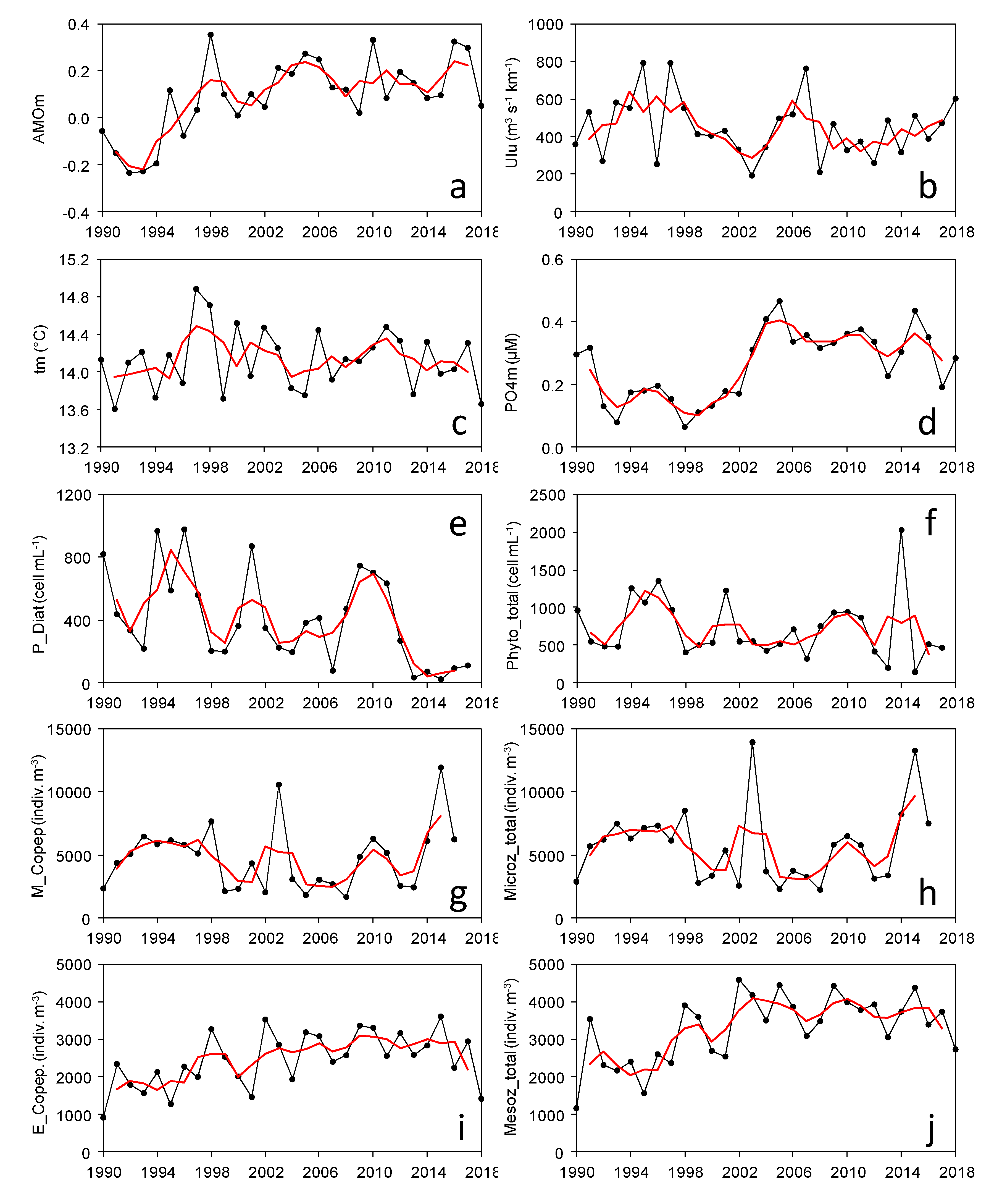
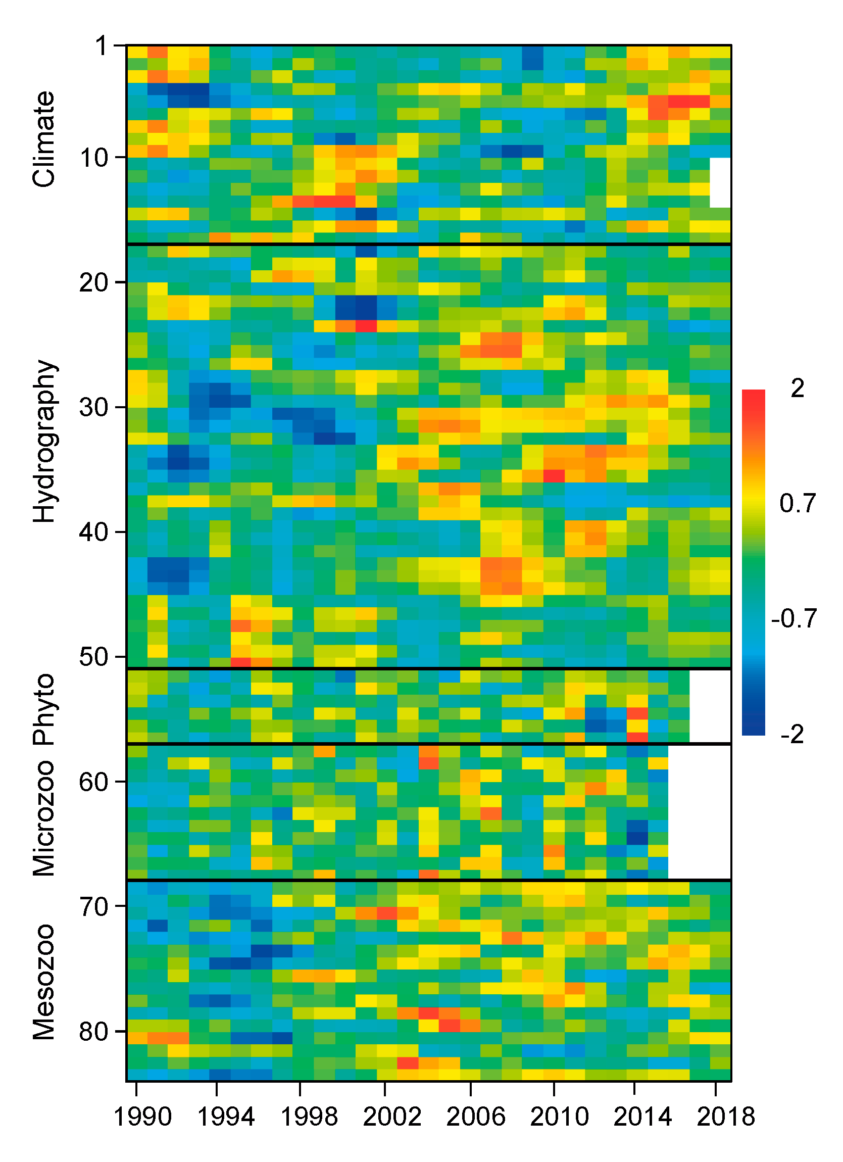
3.1. Multiannual Variability of Series
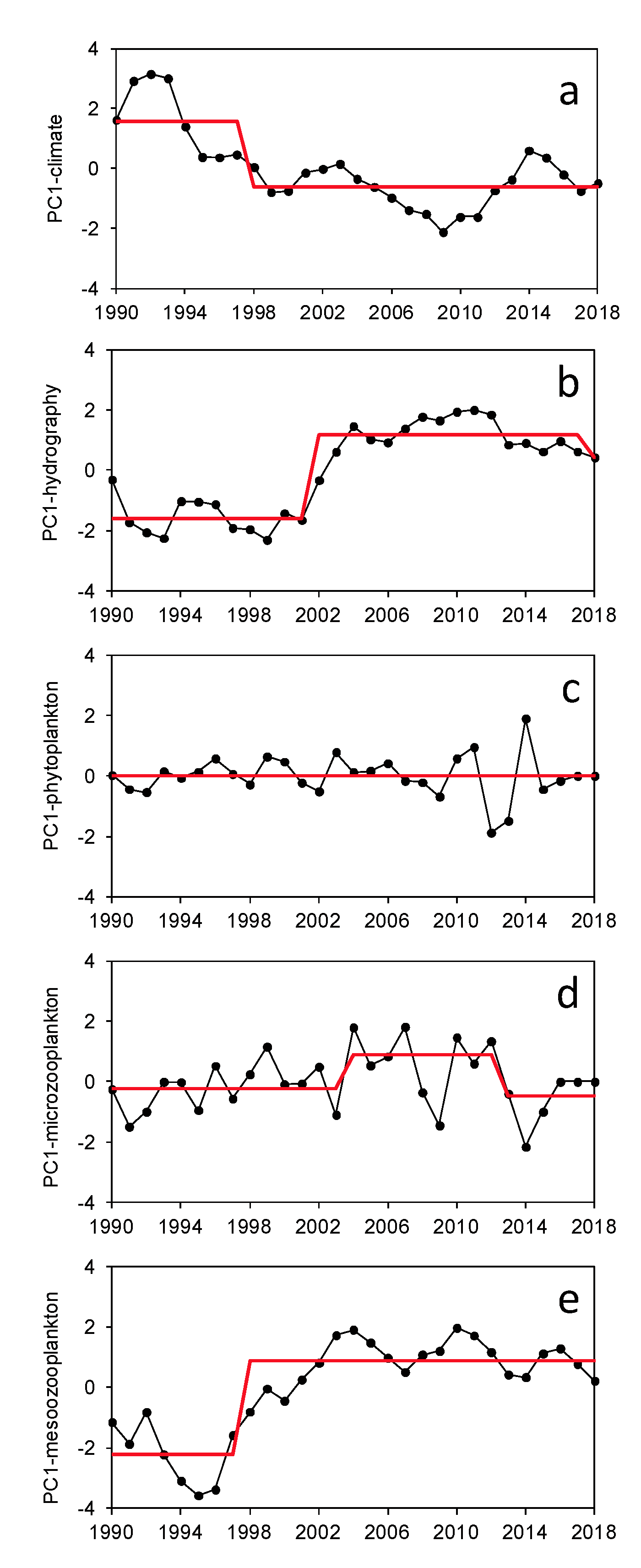
Large year-to-year variability was observed in all series (e.g., selected series in Figure 1), with significant trends in some of them (see Supplementary Tables S1 and S2), which suggests multiannual phases. For instance, there was a significant increase in climatic indices, such as AMO from 1990 to mid-2000, and also rises in GLOTI and SUNSP (Supplementary Table S1). In other cases, there were quasi-decadal oscillations, as observed for UI. In the case of hydrography series, there was a significant increase in phosphate and silicate but a decrease in the mean oxygen concentrations after 2000 (Supplementary Table S1). Moreover, there was a significant rise in primary production throughout the series. Phytoplankton series showed a significant decrease in the total abundance of diatoms, while overall abundance did not show a clear trend (Figure 1). Microzooplankton abundance displayed wide oscillations in total abundance, mainly due to copepods, while other groups (e.g., medusae and Siphonophora) became less abundant. In turn, mesozooplankton showed a clear increase in the abundance of almost all groups, but particularly of copepods, Bivalvia, Euphausiacea, Cladocera, Gastropoda and Chaetognatha, after 2000 (Supplementary Table S1). All series showed relative maxima and minima clustered in periods of several years (Figure 2). For instance, climate series showed positive anomalies at the beginning and end of the 1990s, but some series also showed these anomalies after 2012 (e.g., NAO, AMO, PDO, AO). Most hydrography series changed from negative to positive anomalies around 2002. However, phytoplankton series did not show a clear trend, while microzooplankton series showed a general dominance of positive anomalies after 2002, and almost all mesozooplankton series concentrated positive anomalies after 1998.

3.2. Regime Shifts

The two first components of the PCA accounted for 56.08–66.37% of the total variance for the different series types (Supplementary Table S3). For climatic–meteorological series, the highest correlations with the first component (PC1) included the summer NAO, El Niño index (positive) and AMO, GLOTI and the mean precipitation at A Coruña (negative). For hydrography series, phosphate and silicate concentrations and primary production were the main variables with positive values of correlation with PC1, while oxygen and particulate organic carbon and nitrogen had the highest values of negative correlation. The abundance of flagellates, Cryptophycea and other taxa were the main contributors to the positive values of the PC1 for phytoplankton series, while diatoms and dinoflagellates contributed to negative values. Copepods generally dominated the positive correlations with PC1 for both micro- and mesozooplankton series, the latter showing negative correlations with other groups, such as Foraminifera and Annelida.
Most of the PC1 for each series type showed significant regime shifts (Figure 3). In the case of climate series, the shift was between 1997 and 1998 (p < 0.01), while it was between 2001 and 2002 (p < 0.001) for hydrography series. No shift was found for phytoplankton series. In contrast, microzooplankton showed shifts between 2003 and 2004 (p < 0.05) and between 2012 and 2013 (p < 0.05). One shift between 1997 and 1998 was determined for mesozooplankton series (p < 0.001). Few additional shifts were found for the second principal component (PC2) of all series (Supplementary Table S3, Supplementary Figure S2). For instance, there was a shift in climate PC2 between 2013 and 2014, related to the positive correlations of this component with GLOTI and the negative correlations with SUNSP. Mesozooplankton PC2 (positively correlated with Cnidaria and negatively with Euphausiacea) also showed shifts between 2006 and 2007, and between 2016 and 2017.

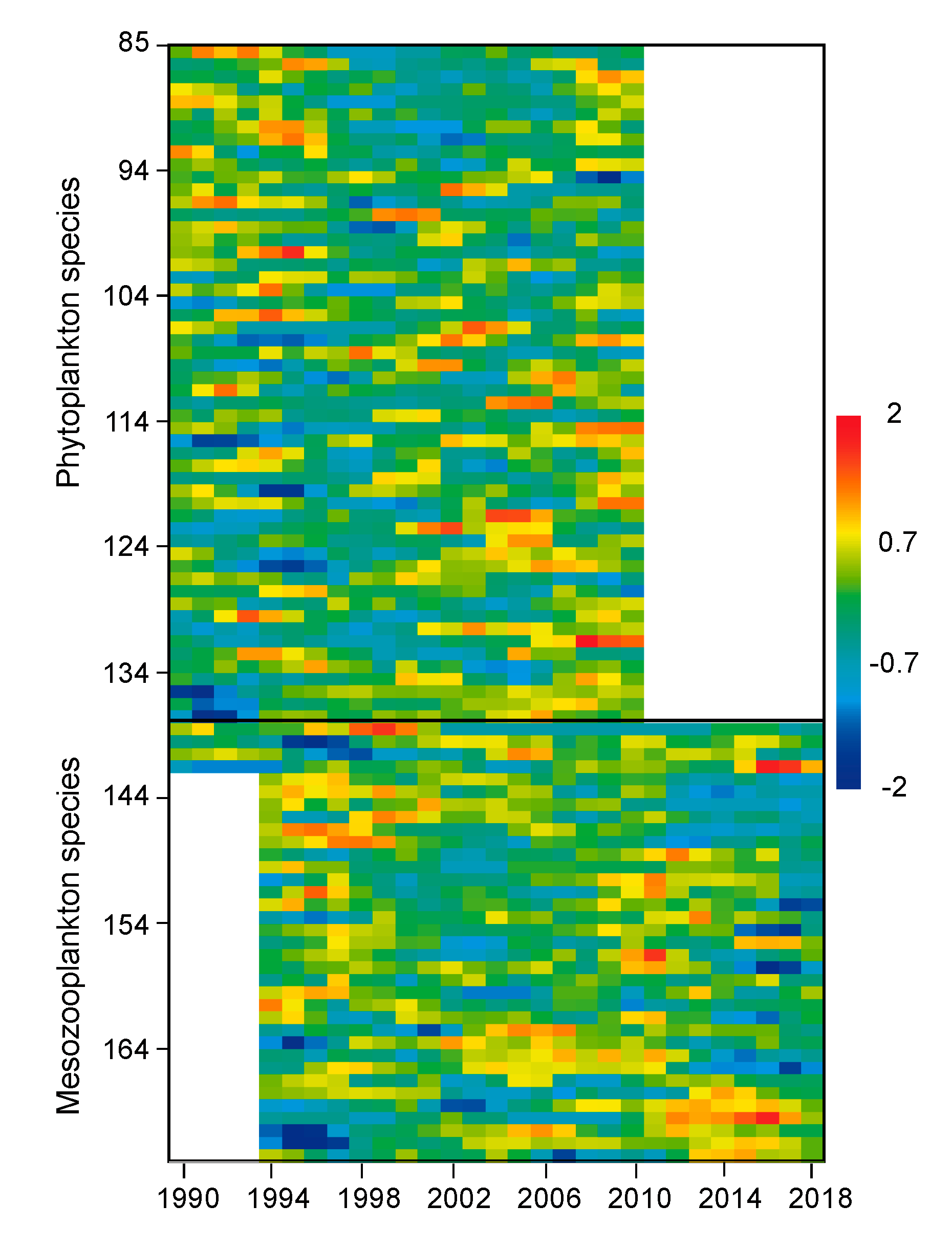
3.3. Regimes in Plankton Species Assemblages

Detailed taxa series showed different patterns among groups of taxa: (Figure 4 and Supplementary Table S2). In the case phytoplankton, positive anomalies prevailed either at the beginning or at the end of the series. Those prevailing mainly at the beginning were mostly diatoms (e.g., Chaetoceros socialis, Ch. gracilis, Ch. decipiens, Lauderia annulata, Skeletonema costatum) but also taxa from Dictyochophyceae (Octactis speculum), dinoflagellates (Tripos lineatus) or Euglenophyceae (Eutreptiella spp.). Those prevailing at the end were dinoflagellates (e.g., Gyrodinium spirale, Heterocapsa niei) but also diatoms (e.g., Pseudo-nitzschia delicatissima, Navicula transitans, other Chaetoceros and Nitzschia spp., Thalassiossira levanderi) and Dictyochophyeace (Dictyocha fibula). For mesozooplankton, positive anomalies clustered before or after approximately 2002. Before 2002, the dominant taxa were Cladocera (Penilia avirostris) and copepods (e.g., Centropages chierchiae, Ctenocalanus vanus, Temora spinifera, T. longicornis). After 2002, there was a change in the dominant taxa of Cladocera (Evadne spinifera) and copepods (e.g., Centropages typicus, Oithona nana, Corycaeus spp.).
For both phytoplankton and mesozooplankton, two main temporal regimes were identified by MDS and cluster analysis (Figure 5 and Supplementary Figure S2). Phytoplankton showed a first regime for the period 1990–1996, correlated positively with climate PC1 and negatively with the first component of the other series. The second phytoplankton regime (1997–2010) was negatively correlated with climate PC1 and positively with the first component of the other series. Diatoms (N. transitans, P. delicatissima, Chaetoceros spp.), dinoflagellates (Torodinium robustum, H. niei), and Dictyochophyceae (D. fibula) were the main taxa that increased from the first to the second regime (Table 1). In turn, taxa with decreasing abundances were mainly diatoms (L. annulata, S. costatum, several spp. of Chaetoceros).
Mesozooplankton regimes spanned the periods 1994–2001 (with a positive correlation with PC1 of climate, and a negative correlation with the other series, except phytoplankton) and 2002–2018 (with negative correlations with climate PC1 and positive correlations with other series, except phytoplankton). The main discriminating taxa for these periods were those increasing their abundance between regimes, such as some copepods (Oithona similis, O. nana) and Cladocera (Podon intermedius, Evadne nordmani), and those decreasing, such as the copepods C. vanus, T. stylifera, T. longicornis, or the Cladocera P. avirostris (Table 2).

4. Discussion

4.1. Regime Shifts in NW Iberia

This study reports, for the first time, multiple regime shifts in plankton assemblages off NW Iberia for the last 29 years. The lack of a long enough series may explain why previous studies in this region focused on continuous trends [22,23,25], or only on some components such as zooplankton [20,21,22], phytoplankton [40], or primary production [24,27]. The new approach revealed a differential influence of climatic and local conditions on plankton assemblages, thus providing a general framework for the changes previously identified not only in this region, but also in the whole NE Atlantic. For instance, our results agree with the observed reorganization of marine ecosystems related to major climate and oceanographic changes after 1990 [7,8,34].
Considering only the first principal component of each series (there were less significant shifts when using the second component), two major types of regime shifts were found in this study. First, the shift between 1997 and 1998 was related to climate and meteorological variables (Figure 6a). Climatic indices for the 1990–1997 period were characterized by relatively low values of AMO, but high values of NAO, ENN and SUNSP, associated to a predominating cold and dry conditions over the NE Atlantic [48,49,50], as indicated by the relatively low precipitation recorded in A Coruña during the spring in this period. Conversely, warm and wet conditions prevailed in the period 1998–2018, when a positive phase of AMO started [51]. In this analysis, the various metrics of the upwelling influence did not show particular correlations with the shift. This result may appear unexpected because of the dependence of the wind regime on major climatic conditions, such as NAO [52]. However, most of the changes in upwelling intensity off Galicia were observed at the seasonal scale (e.g., [44]). For instance, modeling studies found differential changes in upwelling-favorable winds in spring–summer vs. autumn–winter seasons [30], changes that could be largely buffered at the annual scale used in this study. This fact does not imply that upwelling is unimportant in regional oceanography, but simply indicates that its significance is mainly manifested at seasonal and lower time scales, as shown by previous studies [25,29,44].
Second, another type of regime shift was found between 2001 and 2002. In this case, the shift was observed in local oceanographic conditions (Figure 6b). The first period (1990–2001) was characterized by relatively low concentration values of some nutrients, such as phosphate and silicate, and high dissolved oxygen and particulate organic matter, compared with converse conditions in the second period (2002–2018). This suggests either a major oceanographic change (e.g., in the water masses) or enhanced remineralization after 2001. For the Eastern North Atlantic Central Waters (ENACW), the main water mass affected by coastal upwelling in this region, increased inputs of saline and warm subtropical waters in the NE Atlantic have been attributed to negative values of NAO, while cooler and less saline waters prevailed in years of high positive NAO values [53]. These extremes correspond to the southern and northern components of ENACW [54], with the former having a higher proportion of nutrients derived from in situ remineralization than the latter, being more dependent on the mixing depth during winter [55]. This would explain the lower oxygen and organic matter content of waters observed at St. E2CO after 2002, along with changes in the proportion of inorganic nutrients (Figure 2). However, the characteristics of water over the shelf are also affected by processes other than upwelling. For instance, the input of continental waters may alter both thermohaline properties and the nutrient content of shelf waters, particularly in this region because of the high concentrations of some nutrients, such as phosphate and silicate ([28]), both showing a relative excess after 2002 (Figure 2). Such inputs are favored by increased precipitation [56] and a previous study on the primary production series at St. E2CO pointed out the association of rainy periods during the spring, high phosphate concentrations and increased production [27]. Similarly, the analysis of a multidecadal series of zooplankton and precipitation from Vigo (ca. 1° S of Sta. E2CO) found a significant shift in zooplankton assemblages after 2001 related to changes in local precipitation [21]. It is probable that both mechanisms (i.e., change in water masses and variations in runoff) contributed to the observed changes in local oceanography.
Detecting regime shifts, such as those outlined above, is very dependent on the length and quality of the series. One major recommendation is the use of multivariate series, instead of single series, as the former can evidence the interaction of multiple variables [57]. However, even when we have used a collection of multivariate series consistently recorded for nearly three decades, there are several issues that could affect their interpretation. Methodological variations along the recording period can be generally solved through corrections and calibration. For instance, changes in the method for analyzing chlorophyll after 2000 required the application of a correction factor to earlier measurements [27]. In other cases, such as the changes in the experts’ identifications of plankton, there were different solutions. These changes did not affect the abundance counts of major taxa; however, some differences were found in the recognition of phytoplankton (but not zooplankton) species between the different teams of participating experts. For this reason, the analysis of regime shifts in plankton used major taxa (e.g., diatoms, copepods), while the analyses of assemblages were restricted to the species unequivocally recognized for all experts for the longest period available in each case. In addition, there were statistical constraints, mainly related to the significance of the shifts and the length of the regimes than can be detected using a particular time series. The use of principal components, rather than individual variables, allowed for the extraction of the main signal of abrupt change in different types of series and for analyzing their relationships [14,15]. The significance of the shifts in the components was analyzed using a sequential test that enhances its detection at the ends of time series [45]. In addition, the error in the identification due to serial correlation was reduced by estimating and removing the red noise from the series [58]. However, it must be noted that we only analyzed shifts based on abrupt changes in the mean value of the component series, and that different regimes may also result from shifts in the variance and frequency structure [59]. Finally, the series must express a significant proportion of regional variability that can be distinguished from local causes. This is the case of the series observed at the station used in this study, which is well connected to the dynamics of the upwelling transition zone on the NW Iberian coast [20,22,23,24].

4.2. Shifts Related to Climate

The start of a warm period of AMO in 1995 was identified as one of the main drivers of regime shift in many components of the marine ecosystems of the NE Atlantic [31]. Climate-related regime shifts between 1997 and 1999 were reported for plankton in the North Sea [16] and in the Bay of Biscay [15], but were also found in other ecosystem components as pelagic and demersal fish in the North Sea [34] and in Galicia [9], and in birds and cetaceans in the Bay of Biscay [14]. Other studies of plankton series in the NE Atlantic also reported major shifts in this period, but attributed them mainly to changes in local oceanography [60,61,62]. Local conditions also affected plankton regimes detected in this study, as evidenced by their correlations with PC1 of the hydrography series (Figure 5). In any case, even when the exact identification of timing in these multiannual shifts varied according to the series selected and the strength of the coupling between climatic and regional or local oceanographic variables (e.g., [15]), there were similar characteristics shared for the different regimes in all zones.
In this study, the phytoplankton assemblages for the regime prior to 1997 were characterized mainly by chain-forming diatom species, of small individual sizes, and of cylindrical or oval cellular shape. In contrast, after 1997, the characterizing species were from more diverse groups, in addition to diatoms (as dinoflagellates and Dyctiochophyeae), had, in general, larger individual sizes, and more diverse cellular shapes. These characteristics can be assimilated with life traits [60,61] illustrating the different compositions of the assemblages for each regime (Figure 6). Similar results were reported for phytoplankton regimes in the North Sea, where an enlargement in niche size and shifts in niche position were described after 1997, and the dominance of typical cold water species (e.g., S. costatum) in the previous regime [62]. However, despite sharing some characteristics (e.g., dominance of diatoms in cold, low NAO periods), local changes in the coastal regions may be different, as illustrated by the increase in the prymnesiophyte Phaeocystis globosa after 1999 on the Dutch coast ([16]) and the relative decrease in dinoflagellates in other areas [63]. The species composition for the regimes described here was advanced in a previous analysis which was part of the same series, highlighting the diversity of trends in the annual series of individual species [40], and the rapid response of small-sized species (particularly diatoms) to cold water, high-nutrient conditions [61]. A sharp increase in primary production and chlorophyll in the studied station after 1998 was also reported [27].
The climate-related regimes for zooplankton were expressed mainly as a change in the abundance ratio of major groups (Figure 3), rather than individual species. However, climatic effects may have favored the composition of the first regime (1994–2001) for zooplankton species, as suggested by the position of PC1 for climate in Figure 5. Prior to 1998, there was a dominance of holoplanktonic groups (e.g., copepods) over those of meroplankton (e.g., larvae of bivalve and gasteropod mollusks), and a converse situation thereafter. Pronounced changes were also reported for zooplankton in other regions in the NE Atlantic, mainly for copepods. For instance, after 1997, there was a reduction in the total abundance of copepods, due mainly to a decrease in neritic species and a relative increase in small-sized, subtropical species in the North Sea [63,64] and in the Bay of Biscay [15]. All these changes were linked to an enhanced input of warm ocean waters in the period dominated by positive AMO and decreasing NAO conditions, thus pointing to a major role of climate-induced oceanographic processes in the control of zooplankton assemblages, at least at the level of major taxonomic groups. As similar and concurrent shifts were found in upper trophic levels, such as planktivorous fish [7,9], birds and cetaceans [14], these changes are indicative of a major role of bottom-up control of the corresponding regimes described for plankton. A top-down control by their predators (or trophic cascade) cannot be excluded, but this mechanism is more likely to operate in semi-enclosed seas [16].

4.3. Shifts Related to Local-Oceanography

Major shifts in plankton were found for most of the NE Atlantic between 1999 and 2002. Most of them were related to local and sub-regional changes in hydrography and nutrients, but, in contrast to climate-related shifts, all cases reported preferentially affected coastal zones. Changes in phytoplankton included an increase in the most recent regime of at least some species of diatoms (e.g., Pseudo-nitzschia spp.), dinoflagellates, including in other groups (e.g., Phaeocystis globosa) in areas of the North Sea [15,16,64], and also in the English Channel [6,18,19], with noticeable reductions (extensions) in spring (autumn) blooms. There were also reported shifts in zooplankton in this period, mostly related with the increase in coastal locations of small copepods (e.g., Oithona, Oncaea), a decrease in Calanoida, particularly in those of relatively large size (e.g., Paracalanus, Pseudocalanus, Temora), and a general increase in species diversity in areas of the North Sea and the English Channel [6,18,19,64]. In southern regions, such as the Bay of Biscay [26] and Galicia [21] there was an increase in total abundance and biomass. In all reported cases, these shifts were mainly related to local and regional hydrographic conditions.
In our study, the observed shifts in plankton after 2001 were attributed mainly to changes in nutrients and primary production (Figure 6). These shifts appeared in the zooplankton taxa but not in the phytoplankton ones. In the case of microzooplankton, there was a general increase in abundance for all taxa after 2001; however, such an increase was not detected for mesozooplankton general taxa, but for individual species instead. The species increasing their abundance displayed a larger variety of life traits and smaller size than those of the previous regime. The former included ambush-feeding omnivores (O. similis, O. nana, O. media), filter-feeding herbivores (Pseudocalanus elongatus, Podon intermedius, Evadne nordmanni), omnivores (C. typicus), and ambush-feeding carnivores (Corycaeus spp.), according to general trophic classifications (e.g., [65]). Those species with a higher abundance prior to 2002 were, in general, of larger size and with more specialized feeding behaviors, such as filter-feeding herbivores (P. avirostris, T. stylifera, T. longicornis) or omnivores (C. vanus). Similar variations in traits were described for zooplankton series in the North Pacific after the 1997–1998 El Niño [65], thus suggesting that functional diversity may represent a better tracer of community shifts than taxonomic diversity, at least in some ecosystems.

5. Conclusions

The shift in plankton regimes around the turn of the century described in this study implied an increase in complexity of the ecosystem, with a higher number of traits, small-sized species, and a likely increase in diversity. The fact that some of the shifts were mainly related to climate, while others were concurrent with changes in local oceanographic variables, may be due to time lags in the response of the ocean, but also to the particular conditions of the studied sites. For instance, most of the shifts related to changes in currents, nutrients or salinity occurred in coastal zones. This local effect appears to be a characteristic of the response of marine ecosystems to climate change (e.g., [66]), in contrast with terrestrial ecosystems where the effect of climate change may be more direct ([5]). Trophic cascades, however, cannot be discarded as they have been shown to trigger regime shifts in semi-enclosed seas ([16]). In addition, the diversity of variables affecting these shifts supports the hypothesis of a predominant role of non-stationary effects of the climate on oceanographic variables, including plankton ([6]). In this way, the response of the ecosystem would be triggered mainly by the variance in the climate rather than by specific changes in the mean value of a particular index. The recognition of non-stationarity in climate responses would have major implications for future models of climate change, which are currently driven by stationary dynamics (e.g., [67]).
The described regimes appeared synchronized across the NE Atlantic ([7]), and even at larger spatial scales ([17]), supporting the major role of warming and of variations in atmospheric pressure fields on ocean currents and concomitant effects on ecosystems, even when modulated by local factors. The consideration of these biological teleconnections would affect our understanding of the relative importance of climatic vs. local factors in marine ecosystems. Future projections of ecosystem change and management policies (such as the European Marine Strategy Framework Directive) may benefit from considering the diversity of life traits, as a measure of ecosystem complexity, non-stationary effects of climate, and teleconnections across the ocean. All these factors, however, cannot be assessed without the continuation of long-term, multidisciplinary time series of observations, such as the ones used in this analysis.

Supplementary Materials

The following are available online at https://www.mdpi.com/2673-1924/1/4/14/s1, Figure S1: Pearsons’ r correlations between series within each type, Figure S2: Time series of the second principal component of the PCA on each type of series. Figure S3: Cluster of annual series of phytoplankton or mesozooplankton taxa. Table S1: List of original series along with mean, sd and trends. Table S2: List of original series of plankton taxa along with mean, sd and trends. Table S3: Loadings of the first (PC1) and second (PC2) principal components of the PCA for each type of series.

Author Contributions

Conceptualization, A.B.; methodology, A.B., M.Á., M.Á.L., M.R.-V., M.M.V.; formal analysis, A.B.; investigation, L.M.G.G.; data curation, A.B., M.Á., M.Á.L., M.R.-V., M.M.V.; writing—original draft preparation, A.B.; writing—review and editing, A.B., M.Á., L.M.G.G., M.Á.L., M.N.-C., M.R.-V., M.M.V.; visualization, A.B., M.Á.L., M.N.-C.; project administration, A.B.; funding acquisition, A.B., M.R.-V. All authors have read and agreed to the published version of the manuscript.

Funding

This research was funded by the RADIALES project of the Instituto Español de Oceanografia (IEO), with additional funds from the MarRisk project (Interreg POCTEP Spain–Portugal; grant number: 0262 MARRISK 1 E), as well as from the Contrato-Programa Axencia Galega de Innovación (GAIN)-IEO grant (grant number: IN607A 2018/2) of the Axencia Galega de Innovación (GAIN, Xunta de Galicia, Spain).

Acknowledgments

We are grateful for the dedicated work of the many ship crews, technicians, and scientists that made the collection of the time series observations employed in this study possible. Particularly, we thank David Marcote and Ángel F. Lamas (CTD), Nicolás González, Rosario Carballo, and Mónica Castaño (nutrient analysis), Fernando Rozada (POM), Manuel Varela and Jorge Lorenzo (phytoplankton), and Maite Álvarez-Ossorio and Elena Rey (zooplankton) for the initiation and maintenance of the series.

Conflicts of Interest

The authors declare no conflict of interest. The funders had no role in the design of the study; in the collection, analyses, or interpretation of data; in the writing of the manuscript, or in the decision to publish the results.

References

  1. Möllmann, C.; Folke, C.; Edwards, M.; Conversi, A. Marine regime shifts around the globe: Theory, drivers and impacts. Phil. Trans. R. Soc. B 2015, 370. [Google Scholar] [CrossRef] [Green Version]
  2. Conversi, A.; Dakos, V.; Gardmark, A.; Ling, S.; Folke, C.; Mumby, P.J.; Greene, C.; Edwards, M.; Blenckner, T.; Casini, M.; et al. A holistic view of marine regime shifts. Phil. Trans. R. Soc. B 2015, 370. [Google Scholar] [CrossRef] [Green Version]
  3. Reid, P.C.; Edwards, M.; Beaugrand, G.; Skogen, M.; Stevens, D. Periodic changes in the zooplankton of the North Sea during the 20th century linked to oceanic inflow. Fish. Oceanogr. 2001, 12, 260–269. [Google Scholar] [CrossRef] [Green Version]
  4. Beaugrand, G. Long-term changes in copepod abundance and diversity in the North-East Atlantic in relation to fluctuations in the hydroclimatic environment. Fish. Oceanogr. 2003, 12, 270–283. [Google Scholar] [CrossRef]
  5. Hallett, T.B.; Coulson, T.; Pilkington, J.G.; Clutton-Brock, T.H.; Pemberton, J.M.; Grenfell, B.T. Why large-scale climate indices seem to predict ecological processes better than local weather. Nature 2004, 430, 71–75. [Google Scholar] [CrossRef]
  6. Molinero, J.C.; Reygondeau, G.; Bonnet, D. Climate variance influence on the non-stationary plankton dynamics. Mar. Environ. Res. 2013, 89, 91–96. [Google Scholar] [CrossRef]
  7. Alheit, J.; Gröger, J.; Licandro, P.; McQuinn, I.H.; Pohlmann, T.; Tsikliras, A.C. What happened in the mid-1990s? The coupled ocean-atmosphere processes behind climate-induced ecosystem changes in the northeast atlantic and the mediterranean. Deep-Sea Res. II 2019, 159, 130–142. [Google Scholar] [CrossRef]
  8. Möllmann, C.; Conversi, A.; Edwards, M. Comparative analysis of european wide marine ecosystem shifts: A large-scale approach for developing the basis for ecosystem-based management. Biol. Lett. 2011, 7, 484–486. [Google Scholar] [CrossRef] [Green Version]
  9. Kraberg, A.C.; Wiltshire, K.H. Regime shifts in the marine environment: How do they affect ecosystem services. In The Mediterranean Sea: Its History and Present Challenges; Goffredo, S., Dubinsky, Z., Eds.; Springer Science + Business Media: Dordrecht, The Netherlands, 2014; pp. 499–504. [Google Scholar]
  10. Beaugrand, G. The North Sea regime shift: Evidence, causes, mechanisms and consequences. Prog. Oceanogr. 2004, 60, 245–262. [Google Scholar] [CrossRef]
  11. McQuatters-Gollop, A.; Vermaat, J.E. Covariance among North Sea ecosystem state indicators during the past 50 years—Contrasts between coastal and open waters. J. Sea Res. 2011, 65, 284–292. [Google Scholar] [CrossRef]
  12. Peperzak, L.; Witte, H. Abiotic drivers of interannual phytoplankton variability and a 1999–2000 regime shift in the North Sea examined by multivariate statistics. J. Phycol. 2019, 55, 1274–1289. [Google Scholar] [CrossRef] [PubMed]
  13. Cabrero, Á.; González-Nuevo, G.; Gago, J.; Cabanas, J.M. Study of sardine (Sardina pilchardus) regime shifts in the Iberian Atlantic shelf waters. Fish. Oceanogr. 2019, 28, 305–316. [Google Scholar] [CrossRef]
  14. Hemery, G.; D’Amico, F.; Castege, I.; Dupont, B.; D’Elbee, J.; Lalanne, Y.; Mouches, C. Detecting the impact of oceano-climatic changes on marine ecosystems using a multivariate index: The case of the Bay of Biscay (North Atlantic-European ocean). Glob. Chang. Biol. 2008, 14, 27–38. [Google Scholar] [CrossRef]
  15. Luczak, C.; Beaugrand, G.; Jaffré, M.; Lenoir, S. Climate change impact on Balearic shearwater through a trophic cascade. Biol. Lett. 2011, 7, 702–705. [Google Scholar] [CrossRef] [PubMed]
  16. Pershing, A.J.; Mills, K.E.; Record, N.R.; Stamieszkin, K.; Wurtzell, K.V.; Byron, C.J.; Fitzpatrick, D.; Golet, W.J.; Koob, E. Evaluating trophic cascades as drivers of regime shifts in different ocean ecosystems. Phil. Trans. R. Soc. B 2015, 370. [Google Scholar] [CrossRef] [Green Version]
  17. Kröncke, I.; Neumann, H.; Dippner, J.W.; Holbrook, S.; Lamy, T.; Miller, R.; Padedda, B.M.; Pulina, S.; Reed, D.C.; Reinikainen, M.; et al. Comparison of biological and ecological long-term trends related to northern hemisphere climate in different marine ecosystems. Nat. Conserv. 2019, 34, 311–341. [Google Scholar] [CrossRef]
  18. Hernández-Fariñas, T.; Soudant, D.; Barillé, L.; Belin, C.; Lefebvre, A.; Bacher, C. Temporal changes in the phytoplankton community along the French coast of the Eastern English Channel and the Southern Bight of the North Sea. ICES J. Mar. Sci. 2014, 71, 821–833. [Google Scholar] [CrossRef] [Green Version]
  19. Reygondeau, G.; Molinero, J.C.; Coombs, S.; MacKenzie, B.R.; Bonnet, D. Progressive changes in the western English Channel foster a reorganization in the plankton food web. Prog. Oceanogr. 2015, 137, 524–532. [Google Scholar] [CrossRef]
  20. Bode, A.; Alvarez-Ossorio, M.T.; Miranda, A.; Ruiz Villarreal, M. Shifts between gelatinous and crustacean plankton in a coastal upwelling region. ICES J. Mar. Sci. 2013, 70, 934–942. [Google Scholar] [CrossRef] [Green Version]
  21. Buttay, L.; Miranda, A.; Casas, G.; González-Quirós, R.; Nogueira, E. Long-term and seasonal zooplankton dynamics in the northwest Iberian shelf and its relationship with meteo-climatic and hydrographic variability. J. Plankton Res. 2016, 38, 106–121. [Google Scholar] [CrossRef] [Green Version]
  22. Valdés, L.; López-Urrutia, A.; Cabal, J.; Alvarez-Ossorio, M.; Bode, A.; Miranda, A.; Cabanas, M.; Huskin, I.; Anadón, R.; Alvarez-Marqués, F.; et al. A decade of sampling in the Bay of Biscay: What are the zooplankton time series telling us? Prog. Oceanogr. 2007, 74, 98–114. [Google Scholar] [CrossRef]
  23. Bode, A.; Alvarez-Ossorio, M.T.; Cabanas, J.M.; Miranda, A.; Varela, M. Recent trends in plankton and upwelling intensity off Galicia (NW Spain). Prog. Oceanogr. 2009, 83, 342–350. [Google Scholar] [CrossRef]
  24. Bode, A.; Anadón, R.; Morán, X.A.G.; Nogueira, E.; Teira, E.; Varela, M. Decadal variability in chlorophyll and primary production off NW Spain. Clim. Res. 2011, 48, 293–305. [Google Scholar] [CrossRef] [Green Version]
  25. Pérez, F.F.; Padin, X.A.; Pazos, Y.; Gilcoto, M.; Cabanas, M.; Pardo, P.C.; Doval, M.D.; Farina-Bustos, L. Plankton response to weakening of the Iberian coastal upwelling. Glob. Chang. Biol. 2010, 16, 1258–1267. [Google Scholar] [CrossRef] [Green Version]
  26. González-Gil, R.; González Taboada, F.; Höffer, J.; Anadón, R. Winter mixing and coastal upwelling drive long-term changes in zooplankton in the Bay of Biscay (1993-2010). J. Plankton Res. 2015, 37, 337–351. [Google Scholar] [CrossRef]
  27. Bode, A.; Álvarez, M.; Ruíz-Villarreal, M.; Varela, M.M. Changes in phytoplankton production and upwelling intensity off A Coruña (NW Spain) for the last 28 years. Ocean Dyn. 2019. [Google Scholar] [CrossRef] [Green Version]
  28. Alvarez-Salgado, X.A.; Beloso, S.; Joint, I.; Nogueira, E.; Chou, L.; Pérez, F.F.; Groom, S.; Cabanas, J.M.; Rees, A.P.; Elskens, M. New production of the NW Iberian shelf during the upwelling season over the period 1982–1999. Deep Sea Res. 2002, 49, 1725–1739. [Google Scholar] [CrossRef] [Green Version]
  29. Beca-Carretero, P.P.; Otero, J.; Land, P.E.; Groom, S.; Alvarez-Salgado, X.A. Seasonal and inter-annual variability of net primary production in the NW Iberian margin (1998–2016) in relation to wind stress and sea surface temperature. Prog. Oceanogr. 2019, 178. [Google Scholar] [CrossRef]
  30. Casabella, N.; Lorenzo, M.N.; Taboada, J.J. Trends of the Galician upwelling in the context of climate change. J. Sea Res. 2014, 93, 23–27. [Google Scholar] [CrossRef]
  31. Available online: http://www.seriestemporales-ieo.net (accessed on 24 September 2020).
  32. Available online: https://psl.noaa.gov/gcos_wgsp/Timeseries/ (accessed on 30 March 2020).
  33. Available online: https://crudata.uea.ac.uk/cru/data/nao/ (accessed on 25 March 2020).
  34. Edwards, M.; Beaugrand, G.; Helaouet, P.; Alheit, J.; Coombs, S. Marine ecosystem response to the Atlantic multidecadal oscillation. PLoS ONE 2013, 8, e57212. [Google Scholar] [CrossRef] [Green Version]
  35. Available online: https://opendata.aemet.es/ (accessed on 15 March 2020).
  36. González-Nuevo, G.; Gago, J.; Cabanas, J.M. Upwelling index: A powerful tool for marine research in the nw iberian upwelling system. J. Oper. Oceanogr. 2014, 7, 45–55. [Google Scholar] [CrossRef]
  37. Available online: http://www.indicedeafloramiento.ieo.es/ (accessed on 15 March 2020).
  38. Available online: https://doi.org/10.1594/PANGAEA.885413 (accessed on 24 September 2020).
  39. Available online: https://doi.pangaea.de/10.1594/PANGAEA.919082 (accessed on 24 September 2020).
  40. Bode, A.; Estévez, M.G.; Varela, M.; Vilar, J.A. Annual trend patterns of phytoplankton species abundance belie homogeneous taxonomical group responses to climate in the NE Atlantic upwelling. Mar. Environ. Res. 2015, 110, 81–91. [Google Scholar] [CrossRef] [PubMed]
  41. Available online: https://doi.org/10.1594/PANGAEA.908815 (accessed on 24 September 2020).
  42. Available online: https://doi.pangaea.de/10.1594/PANGAEA.919081 (accessed on 24 September 2020).
  43. Available online: https://doi.pangaea.de/10.1594/PANGAEA.919080 (accessed on 24 September 2020).
  44. Nogueira, E.; Perez, F.F.; Rios, A.F. Seasonal patterns and long-term trends in an estuarine upwelling ecosystem (Ria de Vigo, NW Spain). Estuar. Coast. Shelf Sci. 1997, 44, 285–300. [Google Scholar] [CrossRef] [Green Version]
  45. Rodionov, S.N. A sequential algorithm for testing climate regime shifts. Geophys. Res. Lett. 2004, 31. [Google Scholar] [CrossRef] [Green Version]
  46. Clarke, K.R.; Gorley, R.N. Primer V6: User Manual/Tutorial; PRIMER-E Ltd.: Plymouth, UK, 2006; 192p. [Google Scholar]
  47. Hammer, Ø.; Harper, D.A.T.; Ryan, P.D. Past: Paleontological statistics software package for education and data analysis. Palaeontol. Electron. 2001, 4, 9. [Google Scholar]
  48. Folland, C.K.; Knight, J.; Linderholm, H.; Fereday, D.; Ineson, S.; Hurrell, J.W. The summer North Atlantic Oscillation: Past, present and future. J. Clim. 2009, 22, 1082–1103. [Google Scholar] [CrossRef]
  49. López-Parages, J.; Rodríguez-Fonseca, B.; Dommenget, D.; Frauen, C. ENSO influence on the North Atlantic European climate: A non-linear and non-stationary approach. Clim. Dyn. 2016, 47, 2071–2084. [Google Scholar] [CrossRef]
  50. O’Reilly, C.H.; Woollings, T.; Zanna, L. The dynamical influence of the atlantic multidecadal oscillation on continental climate. J. Clim. 2017, 30, 7213–7230. [Google Scholar] [CrossRef]
  51. Knudsen, M.F.; Seidenkrantz, M.-S.; Jacobsen, B.H.; Kuijpers, A. Tracking the atlantic multidecadal oscillation through the last 8000 years. Nat. Commun. 2011, 2. [Google Scholar] [CrossRef]
  52. Marshall, J.; Kushnir, Y.; Battisti, D.; Chang, P.; Czaja, A.; Dickson, R.; Hurrell, J.; McCartney, M.; Saravanan, R.; Visbeck, M. North Atlantic climate variability: Phenomena, impacts and mechanisms. Int. J. Climatol. 2001, 21, 1863–1898. [Google Scholar] [CrossRef]
  53. Prieto, E.; Gonzalez-Pola, C.; Lavin, A.; Holliday, N.P. Interannual variability of the Northwestern Iberia deep ocean: Response to large-scale North Atlantic forcing. J. Geophys. Res. Oceans 2015, 120, 832–847. [Google Scholar] [CrossRef] [Green Version]
  54. Rios, A.F.; Pérez, F.F.; Fraga, F. Water masses in the upper and middle North Atlantic Ocean East of Azores. Deep Sea Res. 1992, 39, 645–658. [Google Scholar] [CrossRef] [Green Version]
  55. Pérez, F.F.; Mouriño, C.; Fraga, F.; Rios, A.F. Displacement of water masses and remineralization rates off the Iberian peninsula by nutrient anomalies. J. Mar. Res. 1993, 51, 869–892. [Google Scholar] [CrossRef] [Green Version]
  56. Otero, P.; Ruiz-Villarreal, M.; Peliz, A. River plume fronts off NW Iberia from satellite observations and model data. ICES J. Mar. Sci. 2009, 66, 1853–1864. [Google Scholar] [CrossRef]
  57. deYoung, B.; Jarre, A. Regime shifts: Methods of analysis. In Encyclopedia of Ocean Sciences; Cochran, J.K., Bokuniewicz, H., Yager, P., Eds.; Academic Press: London, UK, 2019; pp. 489–492. [Google Scholar]
  58. Rodionov, S.N. Use of prewhitening in climate regime shift detection. Geophys. Res. Lett. 2006, 33. [Google Scholar] [CrossRef] [Green Version]
  59. Liu, Q.; Wan, S.; Gu, B. A review of the detection methods for climate regime shifts. Discrete Dyn. Nat. Soc. 2016, 2016. [Google Scholar] [CrossRef] [Green Version]
  60. Litchman, E.; Klausmeier, C.A. Trait-based community ecology of phytoplankton. Annu. Rev. Ecol. Evol. Syst. 2008, 39, 615–639. [Google Scholar] [CrossRef] [Green Version]
  61. Otero, J.; Bode, A.; Álvarez-Salgado, X.A.; Varela, M. Role of functional traits variability in the response of individual phytoplankton species to changing environmental conditions in a coastal upwelling zone. Mar. Ecol. Prog. Ser. 2018, 596, 33–47. [Google Scholar] [CrossRef] [Green Version]
  62. Freund, J.A.; Grüner, N.; Brüse, S.; Wiltshire, K.H. Changes in the phytoplankton community at Helgoland, North Sea: Lessons from single spot time series analyses. Mar. Biol. 2012, 159, 2561–2571. [Google Scholar] [CrossRef] [Green Version]
  63. Alvarez-Fernandez, S.; Lindeboom, H.; Meesters, E. Temporal changes in plankton of the North Sea: Community shifts and environmental drivers. Mar. Ecol. Prog. Ser. 2012, 462, 21–38. [Google Scholar] [CrossRef] [Green Version]
  64. Boersma, M.; Wiltshire, K.H.; Kong, S.M.; Greve, W.; Renz, J. Long-term change in the copepod community in the Southern German Bight. J. Sea Res. 2015, 101, 41–50. [Google Scholar] [CrossRef]
  65. Pomerleau, C.; Sastri, A.R.; Beisner, B.E. Evaluation of functional trait diversity for marine zooplankton communities in the Northeast subarctic Pacific ocean. J. Plankton Res. 2015, 37, 712–726. [Google Scholar] [CrossRef]
  66. Dippner, J.W.; Kornilovs, G.; Junker, K. A multivariate Baltic Sea environmental index. Ambio 2012, 41, 699–708. [Google Scholar] [CrossRef] [PubMed] [Green Version]
  67. Chust, G.; Allen, J.I.; Bopp, L.; Schrum, C.; Holt, J.; Tsiaras, K.; Zavatarelli, M.; Chifflet, M.; Cannaby, H.; Dadou, I.; et al. Biomass changes and trophic amplification of plankton in a warmer ocean. Glob. Chang. Biol. 2014, 20, 2124–2139. [Google Scholar] [CrossRef] [PubMed]
Figure 1. Distribution of annual means of example series for each variable category (climate, hydrography, phytoplankton, microzooplankton, and mesozooplankton). (a): North Atlantic Oscillation (NAOm, relative units), (b): positive monthly values of Upwelling Index (UIu, m3, s−1, km−1), (c): water column temperature (tm, °C), (d): water column phosphate concentration (PO4m, µM), (e): photic zone diatom abundance (P_Diat, cell mL−1), (f): photic zone total phytoplankton abundance (P_Phyto_total, cell mL−1), (g): water column integrated microzooplanktonic copepod abundance (M_Cope, indiv. m−3), (h): water column integrated total microzooplankton abundance (Microz_total, indiv. m−3), (i): water column integrated mesozooplanktonic copepod abundance (E_Cope, indiv. m−3), (j): water column integrated total mesozooplankton abundance (Mesoz_total, indiv. m−3). Red lines indicate 3-year running means.
Oceans 01 00014 g001
Figure 2. Distribution of anomalies from the overall mean for climate, hydrography and plankton series employed in this study. Each series was prefiltered (±3 sd), transformed for normality, normalized, standardized and smoothed using a 3-year running mean (see Methods). Series identification is shown in Supplementary Table S1.
Oceans 01 00014 g002
Figure 3. Time series of the first principal component of the Principal Component Analysis (PCA) on each type of series. (a): Climate series, (b): hydrography series, (c): phytoplankton series, (d): microzooplankton series; (e): mesozooplankton series. The red line indicates the weighed means of the regimes determined with the Rodionov test (see Methods).
Oceans 01 00014 g003
Figure 4. Distribution of anomalies from the overall mean for series of phytoplankton and mesozooplankton species considered in this study. Each series was prefiltered (±3 sd), transformed for normality, normalized, standardized and smoothed using a 3-year running mean (see Methods). Series identification is shown in Supplementary Table S2.
Oceans 01 00014 g004
Figure 5. Plot of the values of the 2 first coordinates of the Non-Metric Multidimensional Analysis (MDS) on the annual series of phytoplankton (a) or mesozooplankton taxa (b). The correlation of the first principal component of the PCA on each type of series is indicated by the length of the vectors. The solid lines enclose the main periods detected by cluster analysis (see Methods).
Oceans 01 00014 g005
Figure 6. Schema of the main properties of the different plankton regimes identified and related to climatic (a) or local oceanography conditions (b). Relative increases (decreases) are indicated by red (blue) arrows.
Oceans 01 00014 g006
Table 1. Main phytoplankton taxa contributing to the separation between periods identified by MDS and cluster analysis. The mean values of abundance (cells mL−1), squared Euclidean distance (D2), the index of discrimination consistency (D2/sd), and the percent contribution (Contr. %) of each taxa to the separation determined by the Similarity Percentages (SIMPER) procedure between periods are given. Relatively low (blue) or high (red) mean abundances are indicated by shading. Series numbers as in Supplementary Table S2.
1990–19972000–2010
Series No.SeriesTaxonomic GroupMean Abund.Mean Abund.D2D2/sdContr. %
116Navicula transitansDiatoms0.330.822.641.615.30
126Pseudo-nitzschia delicatissimaDiatoms3.0012.932.141.164.31
108Chaetoceros spp.Diatoms6.1530.462.091.164.21
136Torodinium robustumDinoflagellates0.200.501.880.933.78
138Heterocapsa nieiDinoflagellates4.058.261.710.903.43
97Lauderia annulataDiatoms4.111.081.601.203.21
101Skeletonema costatumDiatoms42.563.211.571.043.16
120Nitzschia spp.Diatoms0.771.081.520.933.06
110Dictyocha fibulaDictyochophyceae0.050.161.291.022.58
85Bacteriastrum delicatulumDiatoms1.110.041.221.052.45
106Chaetoceros decipiensDiatoms1.150.291.181.042.38
123Prorocentrum balticumDinoflagellates1.034.471.160.852.32
132Thalassiosira levanderiDiatoms0.4920.641.150.682.31
137Gyrodinium spiraleDinoflagellates0.230.391.120.942.25
122Proboscia alataDiatoms0.872.051.110.732.22
92Chaetoceros socialisDiatoms252.08131.831.070.802.16
91Chaetoceros gracilisDiatoms3.562.301.050.842.11
Table 2. Main mesozooplankton taxa contributing to the separation between periods identified by MDS and cluster analysis. The mean values of abundance (cells mL−1), squared Euclidean distance (D2), the index of discrimination consistency (D2/sd), and the percent contribution (Contr. %) of each taxa to the separation determined by the SIMPER procedure between periods are given. Relatively low (blue) or high (red) mean abundances are indicated by shading. Series numbers as in Supplementary Table S2.
1994–20012002–2018
Series No.SeriesTaxonomic GroupMean Abund.Mean Abund.D2D2/sdContr. %
173Oithona similisCopepoda34.12133.022.801.047.63
172Oithona nanaCopepoda8.4827.822.270.926.18
139Penilia avirostrisCladocera0.440.021.871.285.10
140Podon intermediusCladocera66.51126.591.720.864.68
141Evadne nordmaniCladocera25.8983.631.431.013.89
144Ctenocalanus vanusCopepoda28.3714.541.391.213.78
148Temora styliferaCopepoda18.454.751.371.083.74
164Oncaea mediaCopepoda238.55438.451.330.753.62
168Pseudocalanus elongatusCopepoda134.46152.581.291.093.50
170Centropages typicusCopepoda2.879.231.261.203.42
171Corycaeus spp.Copepoda0.121.171.240.843.39
147Temora longicornisCopepoda74.1447.801.210.953.29

