Fisher Information as the Squared Lorentz Factor: Conformal Equivalence of the Bures and Beltrami–Klein Metrics on the Qubit Bloch Ball

Abstract

Three results. (1) We prove the tensor-level conformal identity $d{s}_{\mathrm{BK}}^2=4{\gamma }^2\left(r\right) d{s}_{\mathrm{Bures}}^2$ between the Bures metric and the Beltrami–Klein metric on the open qubit Bloch ball, where ${\gamma }^2\left(r\right)=1/(1-r^2)$ is the squared Lorentz factor. (2) For the visibility coordinate $V=2p-1$ of a binary quantum measurement, the classical Bernoulli Fisher information takes the closed form $I\left(V\right)=1/(1-V^2)={\gamma }^2\left(V\right)$. (3) The conformal structure is special to qubits; for $N\ge 3$, the Bures metric on full-rank density matrices has a non-constant sectional curvature at the maximally mixed state and hence a non-vanishing Weyl tensor and no conformal equivalence to any constant-curvature hyperbolic model (Theorem 2). We outline an experimentally testable operational consequence where sequential non-collinear weak measurements on a qubit predict a Thomas–Wigner rotation with a closed-form purity dependence that deviates from the Pancharatnam baseline at intermediate visibility.

1. Introduction

The qubit Bloch ball is the simplest quantum state space with nontrivial geometric content. It carries two canonical Riemannian metrics from distinct physical principles: the Bures metric, generated by the symmetric logarithmic derivative (SLD) Fisher information, and the Beltrami–Klein metric of hyperbolic 3-space, with which Chen and Ungar [1,2,3,4] identified the gyrovector structure of qubit states. The relationship between these two metrics has not previously been stated at the tensor level. We prove that they are conformally equivalent with a conformal factor equal to the squared Lorentz factor ${\gamma }^2\left(r\right)=1/(1-r^2)$, and this factor coincides with the classical Fisher information of a Bernoulli outcome in the visibility coordinate.

Consider a binary quantum measurement with an outcome probability p. We define the visibility as $V=2p-1\in (-1,1)$, with $V=0$ being a completely random outcome and $\left|V\right|=1$ being a deterministic one. The Fisher information of the Bernoulli model, expressed as V, satisfies

$$I\left(V\right)={\displaystyle \frac{1}{1-V^2}}={\gamma }^2\left(V\right),$$

(1)

with the squared Lorentz factor of special relativity under the identification $V\leftrightarrow \beta$. The present paper shows that Equation (1) is not a coincidence of functional form but reflects a tensor-level conformal structure on the qubit Bloch ball, grounded in the exceptional group isomorphism $\mathrm{SL}(2,\mathbb{C})\cong {\mathrm{Spin}}^{+}(1,3)$.

• Physical interpretation.

Two readings make the identity concrete. Operationally, V is the visibility of a binary measurement, and ${\gamma }^2\left(V\right)$ is its single-shot Fisher information. Thus, the statistical distinguishability of a binary quantum outcome grows with the same functional form that governs relativistic time dilation, with both being fixed by the common group $\mathrm{SL}(2,\mathbb{C})\cong {\mathrm{Spin}}^{+}(1,3)$ acting on the qubit and on spacetime. Dynamically, on a continuously monitored qubit, the unitary part of the evolution acts as a spatial rotation of the Bloch vector, while measurement backaction acts as a Lorentz boost along the measured axis. Therefore, composing two non-collinear weak measurements produces a genuine Thomas–Wigner rotation whose purity dependence (Section 10.3) is the falsifiable content of the framework. The remainder of the paper makes both readings precise and delimits their scope.

Prior work for this journal by Alsing, Cafaro, Felice, and Luongo [5] analyzed the geometric structure of mixed quantum states inside the Bloch sphere, including Bures-related quantities; the present paper is complementary, establishing the tensor-level conformal identity between two natural Bloch ball metrics and its algebraic boundary at $N\ge 3$.

1.1. Scope and Claims

This paper has two central results. First, the Bures metric and the Beltrami–Klein metric on the qubit Bloch ball are conformally equivalent, with a conformal factor ${\gamma }^2\left(r\right)=1/(1-r^2)$ equal to both the squared Lorentz factor and the Fisher information of a binary quantum measurement (Theorem 1, Equation (7)). Second, this conformal structure is special to qubits: for $N\ge 3$, the Weyl tensor of the Bures metric is non-vanishing, an obstruction to conformal equivalence with any constant-curvature model (Theorem 2). Several complementary viewpoints then situate the conformal factor operationally.

• What Is Elementary and What Is New?

We state the elementary content plainly. The identity $I\left(V\right)={\gamma }^2\left(V\right)$ is a one-line reparametrization of the Bernoulli Fisher information, and once both Bloch ball metrics are written in the radial coordinate r, the conformal factor of Theorem 1 is immediate from their ratio. What is not immediate, and what this paper contributes, is twofold. (1) The statement holds at the level of Riemannian metric tensors and not merely distance functions; it fixes all angles, sectional curvatures, volumes, and geodesics at once, which is strictly stronger than the scalar gyrovector identification of Chen and Ungar. (2) The phenomenon has a sharp boundary: it fails for every $N\ge 3$, and the failure is exhibited explicitly by an $\mathfrak{su}\left(3\right)$ sectional-curvature computation at the maximally mixed state (Theorem 2, Appendix A). The single falsifiable prediction of this paper is the purity-dependent Thomas–Wigner rotation of Equation (10).

To our knowledge, the explicit tensor-level conformal identity $d{s}_{\mathrm{BK}}^2=4{\gamma }^2 d{s}_{\mathrm{Bures}}^2$ has not been stated in the existing Bures geometry or gyrovector literatures, where related results appear at the level of either the Bures metric tensor (spherical or Uhlmann hemisphere) or hyperbolic or rapidity formulas for fidelity. The algebraic conformal factor can be inferred once both metrics are written in Bloch coordinates; our contribution is the packaging together with the sharp $N\ge 3$ obstruction and operational consequences. This paper makes no claims about quantum gravity, consciousness, or artificial intelligence.

• Novelty Statement

Building on the seminal identification by Chen and Ungar [1,2,3,4] of the Bloch vector as a gyrovector in the Beltrami–Klein model, this paper extends their algebraic result to the level of Riemannian metrics and establishes the precise algebraic boundary of the phenomenon. Chen and Ungar’s results operate at the scalar- or distance-function level (expressing Bures fidelity through Einstein velocity addition); the present paper establishes the Riemannian tensor-level conformal equivalence, which is strictly stronger. It determines all angles, sectional curvatures, volumes, and the geodesic structure simultaneously. While the individual mathematical ingredients are known, namely the Bernoulli Fisher information (textbook), the isomorphism $\mathrm{SL}(2,\mathbb{C})\cong {\mathrm{SO}}^{+}(1,3)$ (Penrose–Rindler [6]), and the Bloch ball gyrovector structure (Chen–Ungar), the technical contributions are as follows:

(1)

Metric-level conformal identity (qubit): By extending the gyrovector identification of Chen and Ungar from algebra to Riemannian geometry, we show that on the qubit Bloch ball, the Beltrami–Klein metric is conformal to the Bures metric with an explicit factor $d{s}_{\mathrm{BK}}^2=4{\gamma }^2\left(r\right) d{s}_{\mathrm{Bures}}^2$ (Equation (7)).

(2)

Sharp boundary at $\mathit{N}\ge \mathbf{3}$: We prove a conformal obstruction where for $N\ge 3$, the Bures metric is not conformally equivalent to any constant-curvature hyperbolic model, using the Weyl-tensor invariance together with an explicit sectional-curvature non-constancy at the maximally mixed state (Theorem 2).

Secondary clarifications (useful but technically elementary) include the visibility-coordinate identity $I\left(V\right)={\gamma }^2\left(V\right)$ and the Gudermannian relation $arcsin\left(V\right)=\mathrm{gd}(\mathrm{arctanh} V)$ that relates the Fisher–Rao arc-length to rapidity.

1.2. Conventions

• Factor of Four

Throughout, the quantum Fisher information (QFI) denotes the metric $g_{\mu \nu }^{\mathrm{QFI}}$ with $\mathrm{QFI}=4\times$ the Bures metric. We adopt this normalization for two reasons of consistency. First, it is the convention in which the quantum Cramér–Rao bound reads as $\mathrm{Var}(\widehat{\theta })\ge 1/\left(N{F}_Q\right)$ with no extra numerical factor. Second, restricted to pure states, the QFI equals four times the Fubini–Study metric, or equivalently the classical Fisher information metric [7]. Under this choice, the qubit radial QFI is exactly $F_Q\left(r\right)={\gamma }^2\left(r\right)=1/(1-r^2)$, while the Bures radial coefficient is $1/\left[4(1-r^2)\right]={\gamma }^2/4$. Therefore, the conformal identity may be read equivalently as $d{s}_{\mathrm{BK}}^2=4{\gamma }^2 d{s}_{\mathrm{Bures}}^2$ or $d{s}_{\mathrm{BK}}^2={\gamma }^2 d{s}_{\mathrm{QFI}}^2$. Every place the factor of four enters is flagged in situ.

• Conformal Relation

The central metric result $d{s}_{\mathrm{BK}}^2=4{\gamma }^2·d{s}_{\mathrm{Bures}}^2$ uses the Bures metric. Equivalently, $d{s}_{\mathrm{BK}}^2={\gamma }^2·d{s}_{\mathrm{QFI}}^2$.

• Notation

V = visibility $=2p-1\in (-1,1)$ (open interval; regularity conditions exclude $V=\pm 1$ where Fisher information diverges). $r=\left|\overrightarrow{r}\right|$ = the Bloch ball radial coordinate $=\left|V\right|$ for the 1D Bernoulli manifold. $\xi =\mathrm{arctanh}\left(V\right)$ = rapidity. $\gamma =1/\sqrt{1-V^2}$ = the Lorentz factor. $I\left(V\right)={\gamma }^2\left(V\right)$ throughout.

2. The Identity: Complete Derivation

2.1. Classical Fisher Information

For a Bernoulli distribution with a parameter $p\in (0,1)$, the Fisher information is $I\left(p\right)=1/\left[p\right(1-p\left)\right]$. Reparameterizing via $p=(1+V)/2$ with Jacobian $dp/dV=1/2$ yields

$$I\left(V\right)=I\left(p\right)·{\left({\displaystyle \frac{dp}{dV}}\right)}^2={\displaystyle \frac{1}{p(1-p)}}·{\displaystyle \frac{1}{4}}={\displaystyle \frac{4}{1-V^2}}·{\displaystyle \frac{1}{4}}={\displaystyle \frac{1}{1-V^2}}={\gamma }^2\left(V\right).$$

(2)

2.2. Quantum Fisher Information

For a qubit state $\rho =(I+\overrightarrow{r}·\overrightarrow{\sigma })/2$ with a Bloch vector $\overrightarrow{r}$, the quantum Fisher information with respect to the radial parameter $r=\left|\overrightarrow{r}\right|$ is

$$F_Q\left(r\right)={\displaystyle \frac{1}{1-r^2}}={\gamma }^2\left(r\right).$$

(3)

This equals $4\times$ the Bures metric radial coefficient: $g_{rr}^{\mathrm{Bures}}=1/\left[4(1-r^2)\right]={\gamma }^2/4$.

3. The Geometry: Spherical Information, Hyperbolic Kinematics

3.1. The Classical 1D Bernoulli Manifold

The Fisher–Rao line element on the 1D Bernoulli manifold parameterized by V is

$$d{s}_{\mathrm{FR}}^2=I\left(V\right) d{V}^2={\displaystyle \frac{d{V}^2}{1-V^2}}.$$

(4)

The Fisher–Rao geodesic distance from $V=0$ to V is $d_{\mathrm{FR}}(0,V)=arcsin\left(V\right)$. When writing this spherical arc length as $\theta$ and the rapidity as $\xi =\mathrm{arctanh}\left(V\right)$, the two are related through the Gudermannian function by

$$\theta =\mathrm{gd}\left(\xi \right),sin\theta =tanh\xi =V,\mathrm{equivalently}\theta =arcsin\left(V\right).$$

Thus, $\theta$ is the spherical distance whose sine is the visibility V, and $\xi$ is the hyperbolic (rapidity) distance; the Gudermannian maps one onto the other.

3.2. The Bloch Ball with the QFI Metric

The Bures metric on the interior of the Bloch ball $B^3=\{r<1\}$ is

$$d{s}_{\mathrm{Bures}}^2={\displaystyle \frac{d{r}^2}{4(1-r^2)}}+{\displaystyle \frac{r^2}{4}} d{\mathsf{\Omega }}^2,$$

(5)

where $d{\mathsf{\Omega }}^2=d{\theta }^2+{sin}^2\theta d{\varphi }^2$. This is the round metric on the northern hemisphere of $S^3$ of a radius ${\displaystyle \frac{1}{2}}$ (constant positive sectional curvature $K=+4$), identified with the interior of the Bloch ball via $r=sin\chi$. The Bures geodesic distance from the center to the radius r is $d_{\mathrm{Bures}}(0,r)={\displaystyle \frac{1}{2}}arcsin\left(r\right)$; equivalently, the QFI geodesic distance is $d_{\mathrm{QFI}}(0,r)=arcsin\left(r\right)$.

3.3. The Beltrami–Klein Metric on the Bloch Ball

The Beltrami–Klein model of the hyperbolic 3-space $H^3$ on the same open ball $B^3$ is

$$d{s}_{\mathrm{BK}}^2={\displaystyle \frac{d{r}^2}{{(1-r^2)}^2}}+{\displaystyle \frac{r^2}{1-r^2}} d{\mathsf{\Omega }}^2.$$

(6)

This has a constant negative sectional curvature $K=-1$. The geodesic distance is $d_{\mathrm{BK}}(0,r)=\mathrm{arctanh}\left(r\right)$.

3.4. The Conformal Equivalence

Theorem 1

(Conformal equivalence on the qubit Bloch ball). On the open Bloch ball $B^3=\{r<1\}$, the Beltrami–Klein metric is conformally equivalent to the Bures metric with a conformal factor $4{\gamma }^2\left(r\right)=4/(1-r^2)$:

$$d{s}_{\mathrm{BK}}^2=4{\gamma }^2\left(r\right)·d{s}_{\mathrm{Bures}}^2.$$

(7)

Equivalently, $d{s}_{\mathrm{BK}}^2={\gamma }^2·d{s}_{\mathrm{QFI}}^2$.

Proof. 

Dividing Equation (6) by Equation (5) component-wise yields

$$\begin{array}{cc}\hfill \text{Radial:}& {\displaystyle \frac{d{r}^2/{(1-r^2)}^2}{d{r}^2/\left[4(1-r^2)\right]}}={\displaystyle \frac{4}{1-r^2}}=4{\gamma }^2\left(r\right),\hfill \\ \hfill \text{Angular:}& {\displaystyle \frac{r^2 d{\mathsf{\Omega }}^2/(1-r^2)}{r^2 d{\mathsf{\Omega }}^2/4}}={\displaystyle \frac{4}{1-r^2}}=4{\gamma }^2\left(r\right).\hfill \end{array}$$

Both components yield the same factor; the relation is therefore a genuine conformal equivalence of Riemannian metrics and not a coordinate identification. □

Remark 1

(Ricci flow context). The Beltrami–Klein metric $g_{\mathrm{BK}}$, being Einsteinian with $\mathrm{Ric}\left(g_{\mathrm{BK}}\right)=-2g_{\mathrm{BK}}$, is a fixed point of volume-normalized Ricci flow. In three dimensions, the Weyl tensor vanishes identically, and conformal flatness is controlled by the Cotton tensor; our conformal relation Equation (7) is an explicit global identity and not an automatic consequence of the dimension. This perspective also illuminates the $N\ge 3$ obstruction: in dimensions $\ge 4$, the non-vanishing Weyl tensor provides a conformal invariant that obstructs equivalence to constant-curvature models.

4. Six Complementary Perspectives

4.1. Dependency Structure

The six perspectives are complementary viewpoints rather than strictly independent derivations. Perspectives 2–5 are closely related representations of the same underlying structure (the Bloch or gyrovector picture and the $\mathrm{SL}(2,\mathbb{C})\cong {\mathrm{SO}}^{+}(1,3)$ correspondence), while Perspectives 1 and 6 provide operational and information-geometric context. We order them by historical lineage and increasing abstraction.

4.2. Perspective 1: Stokes–Minkowski Polarization Optics

The Stokes parameters $(S_0,S_1,S_2,S_3)$ form a Minkowski four-vector. Mueller matrices preserving the Stokes cone are Lorentz transformations. For a degree of polarization $V=\left|\overrightarrow{S}\right|/S_0$, the transformation from unpolarized to polarized is a Lorentz boost with $\beta =V$, yielding $I\left(V\right)={\gamma }^2\left(V\right)$.

4.3. Perspective 2: Bloch Ball Gyrovector Algebra

Chen and Ungar [1,3] proved that Bloch vectors are composed via Einstein velocity addition. Chen, Fu, Ungar, and Zhao [8] provided the rapidity parametrization and hyperbolic-triangle interpretation of Bures fidelity. The Bloch ball under this composition is a gyrovector space, the natural algebraic framework for hyperbolic geometry. The identification $V\leftrightarrow \beta$ is an algebraic isomorphism.

4.4. Perspective 3: SLD Quantum Fisher Information

The symmetric logarithmic derivative (SLD) Fisher information for a qubit state gives $F_Q\left(r\right)=1/(1-r^2)={\gamma }^2\left(r\right)$. This is the Petz-distinguished monotone metric [9]. Under the Petz classification, the SLD (Bures) metric is the minimal element in the family of quantum monotone metrics; it gives the tightest quantum Cramér–Rao bound and is operationally optimal for quantum state estimation.

4.5. Perspective 4: Burns–Greenfield–Dressel Measurement Dynamics

Burns, Greenfield, and Dressel [10] established that the combined group of unitary evolution and non-unitary measurement backaction on a continuously monitored qubit is $\mathrm{SL}(2,\mathbb{C})$: unitary rotations → spatial rotations in $\mathrm{SO}\left(3\right)$; measurement-induced state changes → Lorentz boosts. We cite Burns, Greenfield, and Dressel for the $\mathrm{SL}(2,\mathbb{C})$/Lorentz group action correspondence; our metric identity is independent. The measurement strength maps to rapidity $\xi =\mathrm{arctanh}\left(V\right)$.

4.6. Perspective 5: Chentsov Uniqueness and the Petz Classification

Proposition 1

(Chentsov necessity of the ${\gamma }^2$ form). Let g be any Riemannian metric on the Bernoulli manifold $\mathcal{B}=\left\{\mathrm{Bernoulli}\right(p):p\in (0,1\left)\right\}$ that is invariant under Markov morphisms and expressed in the visibility coordinate $V=2p-1$. Then, $g=c·d{V}^2/(1-V^2)$ for some constant $c>0$, with the standard normalization $c=1$, $I\left(V\right)={\gamma }^2\left(V\right)$.

At the quantum level, the Petz classification [9] identifies a continuous family of monotone metrics. The SLD (Bures) metric is the minimal element, operationally optimal for quantum estimation via the quantum Cramér–Rao bound.

4.7. Perspective 6: Cramér–Rao Bound

The quantum Cramér–Rao bound gives $\mathrm{Var}\left(\widehat{V}\right)\ge 1/[N·F_Q\left(V\right)]$. Substituting $F_Q\left(V\right)={\gamma }^2\left(V\right)$ yields

$$\mathrm{Var}\left(\widehat{V}\right)\ge {\displaystyle \frac{1-V^2}{N}}={\displaystyle \frac{1}{N {\gamma }^2\left(V\right)}}.$$

(8)

As $V\to 1$, the estimator variance $(1-V^2)/N$ trends toward zero, and thus the precision improves without bound; the qubit Cramér–Rao bound is saturable via maximum-likelihood estimation.

Remark 2

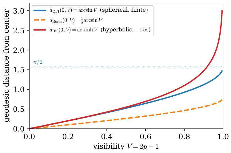
(Coordinate nature of the divergence). It is important to separate two distances. The Mandelstam–Tamm speed limit $\tau \ge \pi \hslash /(2\Delta E)$ measures state evolution in the Bures metric [11,12], and the Bures (equivalently Fisher–Rao) distance from the center of the ball to its boundary is finite, where $d_{\mathrm{QFI}}(0,r)=arcsin\left(r\right)\to \pi /2$ and $d_{\mathrm{Bures}}(0,r)\to \pi /4$ as $r\to 1$. A pure state is therefore reached and distinguished from an orthogonal pure state in a finite time. What diverges is only the Beltrami–Klein (hyperbolic) distance $\mathrm{artanh}\left(r\right)\to \infty$, and it does so because the Beltrami–Klein model represents hyperbolic space on a bounded ball whose boundary $r=1$ sits at an infinite hyperbolic radius. The relation $d{s}_{\mathrm{BK}}=2\gamma d{s}_{\mathrm{Bures}}$ shows the conformal factor rescaling arc length between the two representations. The $\gamma \to \infty$ behavior near purity is thus a property of the hyperbolic coordinate mapping and not a physical restriction on state transitions. Figure 1 makes the contrast explicit.

5. The Group-Theoretic Bridge

5.1. The Isomorphism

The special linear group $\mathrm{SL}(2,\mathbb{C})$ is the double cover of the proper orthochronous Lorentz group: $\mathrm{SL}(2,\mathbb{C})\cong {\mathrm{Spin}}^{+}(1,3)$. This is a textbook result (Penrose–Rindler [6], Ch. 1). Qubit states transform under $\mathrm{SL}(2,\mathbb{C})$; unitary operations ($\mathrm{SU}\left(2\right)\subset \mathrm{SL}(2,\mathbb{C})$) are spatial rotations, and non-unitary operations are boosts.

5.2. Invariant Content

The invariant content of $I\left(V\right)={\gamma }^2$ is that the Chentsov-unique Fisher–Rao metric on the Bernoulli manifold, expressed in the coordinate that $\mathrm{SL}(2,\mathbb{C})$ identifies as a velocity-like parameter, takes the form of the squared Lorentz factor. Both sides are determined by the same group.

5.3. What the Identity Does Not Claim

The identity does not claim (1) that the qubit state space “is” Minkowski spacetime; (2) that measurement “causes” relativistic effects; (3) that Fisher information replaces the energy–momentum tensor; or (4) that the correspondence extends to gravitational physics.

5.4. The Curvature Clarification

The Bures metric on the 3D Bloch ball has constant sectional curvature $K=+4$ (hemisphere of $S^3$ with a radius of ${\displaystyle \frac{1}{2}}$); equivalently, the QFI metric (= $4 \times$ Bures) has $K=+1$. The Beltrami–Klein metric has $K=-1$ ($H^3$). The correspondence operates at the 1D level (no curvature ambiguity) and at the group level. The 3D metrics are related by conformal equivalence (Equation (7)) and not isometry. The Gudermannian function provides the bridge; with $\theta =\mathrm{gd}\left(\xi \right)$ and $sin\theta =tanh\xi =V$, the hyperbolic geodesic distance $\xi =\mathrm{artanh}\left(V\right)$ and the spherical geodesic distance $\theta =arcsin\left(V\right)$ are Gudermannian conjugates.

6. The Measurement–Relativity Dictionary

Table 1. Measurement–relativity dictionary.

Measurement Domain	Relativity Domain	Bridge
Visibility V	Velocity $\beta$	$V\leftrightarrow \beta$
Fisher info $I\left(V\right)$	${\gamma }^2$	Equation (1)
Rapidity ${\xi }_{\mathrm{meas}}$	$\xi =\mathrm{arctanh}\left(\beta \right)$	Identical
Bures metric (spherical)	–	Equation (5)
Beltrami–Klein	Velocity space	Equation (6)
Conformal factor $4{\gamma }^2$	–	Equation (7)
Sequential measurements	Boost composition	Thomas–Wigner
$\mathrm{SL}(2,\mathbb{C})$ on Bloch ball	${\mathrm{Spin}}^{+}(1,3)$ on spacetime	Exceptional isomorphism

collects the correspondences established in the preceding sections, pairing each measurement-domain quantity with its relativistic counterpart and with the equation that links them.

7. Cross-Domain Convergence: Optics and Two-Band Systems

The identity $I\left(V\right)={\gamma }^2\left(V\right)$ is not isolated. Two well-established lines of physics realize the same $\mathrm{SL}(2,\mathbb{C})$/Lorentz/${\gamma }^2$ structure on genuine two-level or two-mode systems, where the correspondence is exact rather than analogical.

7.1. Quantum Optics: Squeezing During a Lorentz Boost

Han, Kim, and Noz [13] established that squeeze operators generate $\mathrm{SU}(1,1)\cong \mathrm{SO}(2,1)$ transformations, the 2+1D Lorentz group. In $\mathrm{SU}(1,1)$ interferometry [14], QFI for phase estimation scales as ${\gamma }^2$. LIGO’s squeezed vacuum injection [15] is a Lorentz boost on the vacuum state.

7.2. Condensed Matter: Quantum Geometric Tensor

Zanardi, Giorda, and Cozzini [16] proved that fidelity susceptibility diverges as the QFI metric coefficient at its quantum phase transitions. For two-band systems, this takes the ${\gamma }^2$ form.

• Summary.

Both lines realize the same ${\gamma }^2$ or $\mathrm{SL}(2,\mathbb{C})$/Lorentz structure on genuine two-level or two-mode systems. The identity $I\left(V\right)={\gamma }^2\left(V\right)$ is the compact algebraic signature common to them.

8. Relationship to Concurrent and Prior Work

• Relativistic and Entropic Aspects of Qubit States

The relativistic and entropic properties of qubit and Bloch ball states have an established body of research. The non-covariance of the reduced spin entropy under Lorentz boosts was established by Peres, Scudo, and Terno [17], and the operational meaning of the spin qubit in the relativistic regime was developed through the quantum reference frame program of Giacomini, Castro-Ruiz, and Brukner [18,19] and Apadula, Castro-Ruiz, and Brukner [20], with related constructions by Palge and Dunningham [21]. Entropic and entanglement measures for qubit states were treated by Wilde [22], Wootters [23], Mintert, and Buchleitner [24] and Berta, Christandl, Colbeck, Renes, and Renner [25]. The present paper is complementary; it contributes the tensor-level conformal identity between the Bures and Beltrami–Klein metrics and its sharp boundary at $N\ge 3$, rather than a statement about Lorentz transformations of encoded information.

• Relational QM and Quantum Reference Frames

The visibility parameter V is inherently relational, i.e., defined relative to a measurement basis and an observer. Adlam and Rovelli [26] argued that “information is physical” in the context of cross-perspective links, and Di Biagio and Rovelli [27] formalized relative information using Shannon theory. The identity $I\left(V\right)={\gamma }^2\left(V\right)$ provides a complementary geometric structure on this space of relative information states. Giacomini, Castro-Ruiz, and Brukner [18] showed that QM remains covariant under QRF changes, and Apadula et al. [20] extended this to Lorentz symmetry. Perche and Martín-Martínez [28] showed that spacetime geometry can be recovered from quantum measurements. The conformal mapping in Equation (7) can be interpreted as the information-geometric counterpart of switching between informational and kinematic descriptions.

9. Addressing Potential Objections

9.1. “It’s Just a Jacobian or Coordinate Artifact”

The identity $I\left(V\right)={\gamma }^2\left(V\right)$ is the Chentsov-unique metric coefficient in the visibility coordinate (Proposition 1). The choice of V is physically selected by the $\mathrm{SL}(2,\mathbb{C})$ group structure.

9.2. “The Fisher Metric Has the Wrong Signature”

The Fisher metric is positive-definite (Riemannian); the Minkowski metric is indefinite. The results operate at three levels: the group level ($\mathrm{SL}(2,\mathbb{C})$ generates both), the 1D metric level ($I\left(V\right)={\gamma }^2$), and the conformal level. At none of these does the signature play a role. Whether a Lorentzian extension exists is an open structural question for future work.

9.3. “Both Spaces Are Spherical, So Where’s the SR Connection?”

This was addressed in Section 5.4. The 3D geometries are not isometric. The correspondence operates at the 1D level and group level; the 3D metrics are related by conformal equivalence (Equation (7)).

9.4. “This Only Works for Qubits”

This is true as stated. However, (1) binary outcome measurements are ubiquitous and operationally natural (threshold detectors and yes or no POVMs); (2) many physical settings reduce to effective qubits (two-band Hamiltonians, polarization optics, with spin-${\displaystyle \frac{1}{2}}$ subspaces); and (3) the obstruction itself provides a precise boundary statement for when constant-curvature hyperbolic models fail.

Theorem 2

(Conformal non-equivalence for $N\ge 3$). For N-level quantum systems with $N\ge 3$, the Bures metric on the space of full-rank density matrices is not conformally equivalent to the Beltrami–Klein metric on any d-dimensional hyperbolic ball ($d=N^2-1$).

Proof. 

The argument proceeds in five steps.

Step 1 (Conformal invariance of the Weyl tensor). The Beltrami–Klein metric on $B^d$ has a constant sectional curvature $K=-1$ and hence a vanishing Weyl tensor $W=0$. For $d\ge 4$, the $(1,3)$-Weyl tensor is a conformal invariant [29] where if $g_1={\mathsf{\Omega }}^2{g}_2$, then $W\left(g_1\right)=W\left(g_2\right)$. Since $d=N^2-1\ge 8$ for $N\ge 3$, conformal equivalence would force $W\left(g_B\right)=0$.

Step 2 (Einstein condition at the maximally mixed state). At ${\rho }_{*}=I/N$, the group $\mathrm{SU}\left(N\right)$ acts on $T_{{\rho }_{*}}{\mathcal{D}}_N^{\circ }\cong \mathfrak{su}\left(N\right)$ via the adjoint representation, which is irreducible (since $\mathfrak{su}\left(N\right)$ is simple; equivalently, the only $\mathrm{Ad}$-invariant bilinear forms on $\mathfrak{su}\left(N\right)$ are multiples of the Killing form). Both $g_B$ and $\mathrm{Ric}$ are $\mathrm{SU}\left(N\right)$-invariant symmetric $(0,2)$ tensors. Thus, under Schur’s lemma, $\mathrm{Ric}\left({\rho }_{*}\right)=\lambda g_B\left({\rho }_{*}\right)$ for some $\lambda \in \mathbb{R}$.

Step 3 (Einstein + $\mathit{W}\mathbf{=}\mathbf{0}$ forces constant curvature). At any Einstein point ($\mathrm{Ric}=\lambda g$) with $W=0$, the standard decomposition of the Riemann tensor reduces to $R={\displaystyle \frac{\lambda }{d-1}} g\overline{)\wedge }g$, the curvature tensor of a space of a constant sectional curvature [29].

Step 4 (Nonconstant sectional curvature). Dittmann [30] proved that for $N>2$, the Bures manifold of nonsingular density matrices is not of a constant curvature and not locally symmetric. Dittmann [31] further showed that the curvature diverges near lower-rank boundaries. We verify non-constancy at ${\rho }_{*}$ explicitly via the O’Neill submersion formula [32], carried out in full in Appendix A. Since the Bures metric arises from the Riemannian submersion $\pi :S^{2N^2-1}\to {\mathcal{D}}_N^{\circ }$, $\pi \left(W\right)=W{W}^{†}$ [33], the sectional curvature at ${\rho }_{*}$ for Bures-orthonormal $X,Y\in T_{{\rho }_{*}}{\mathcal{D}}_N^{\circ }$ is

$$K_B(X,Y)=1+{\displaystyle \frac{3N^3}{64}}\left[-\mathrm{Tr}\left({[X,Y]}^2\right)\right].$$

(9)

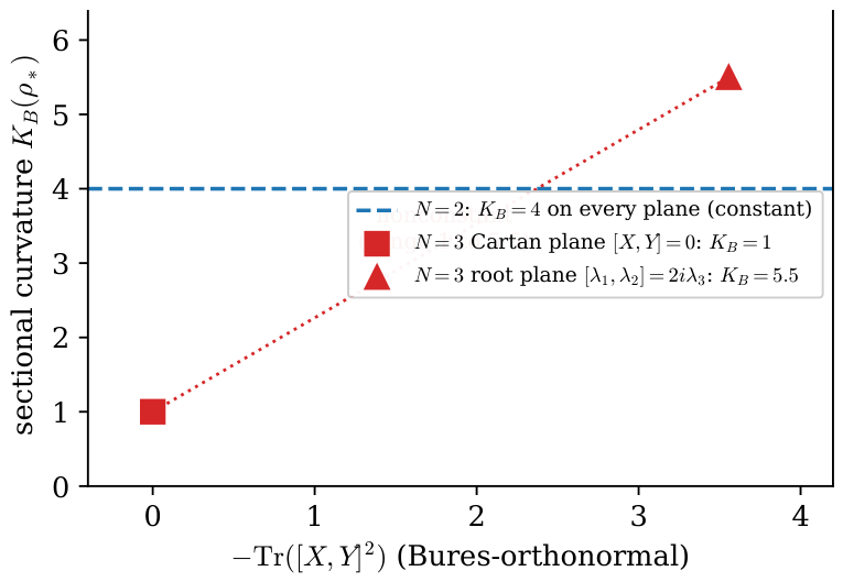
For $N=3$, the Cartan (commuting) plane $[{\lambda }_3,{\lambda }_8]=0$ gives $K_B=1$, while the root plane $[{\lambda }_1,{\lambda }_2]=2i{\lambda }_3$ gives $K_B=11/2$. The two values at the same point ${\rho }_{*}$ are computed explicitly in Appendix A. Hence, the sectional curvature at ${\rho }_{*}$ is not constant.

Step 5 (Contradiction via Riemann decomposition). At the Einstein point ${\rho }_{*}$, the Schouten tensor takes the form $S={\displaystyle \frac{\lambda }{2(d-1)}}{g}_B$, and thus its Kulkarni–Nomizu contribution to the Riemann tensor is $S\overline{)\wedge }g={\displaystyle \frac{\lambda }{d-1}}{g}_B\overline{)\wedge }{g}_B$. The standard decomposition $R=W+S\overline{)\wedge }g$ then yields $W=R-{\displaystyle \frac{\lambda }{d-1}}{g}_B\overline{)\wedge }{g}_B$. If $W\left({\rho }_{*}\right)=0$, then the Riemann tensor at ${\rho }_{*}$ would reduce to $R={\displaystyle \frac{\lambda }{d-1}}{g}_B\overline{)\wedge }{g}_B$, and the curvature tensor of a constant sectional curvature $K=\lambda /(d-1)$. However, Step 4 establishes that sectional curvatures at ${\rho }_{*}$ are not all equal. Therefore, $W\left(g_B\right)\left({\rho }_{*}\right)\ne 0$, contradicting the conformal equivalence assumption from Step 1. □

For $N=2$, every pair of Pauli matrices yields $K_B=4$ (constant curvature), consistent with the Uhlmann hemisphere ${\displaystyle \frac{1}{2}}{S}^3$ [33]. The Weyl tensor vanishes identically in dimension three, and thus no obstruction arises. Figure 2 contrasts the qubit and qutrit cases at the maximally mixed state.

9.5. The One–to–Two Dimension Jump in the Invariant Curvature Space

The obstruction has a clean representation-theoretic origin. An $\mathrm{SU}\left(N\right)$-invariant algebraic curvature tensor on $\mathfrak{su}\left(N\right)$ must be assembled from the invariant structures the algebra provides. Two are available: the Killing form, which builds the constant-curvature tensor

$$R_1(X,Y,Z,W)=\langle X,Z\rangle \langle Y,W\rangle -\langle X,W\rangle \langle Y,Z\rangle \left(\mathrm{from}g\overline{)\wedge }g\right),$$

and the commutator pairing $R_2(X,Y,Z,W)=\langle [X,Y],[Z,W]\rangle$. For $\mathfrak{su}\left(2\right)$ the Jacobi/Lagrange identity forces $R_2$ to be a fixed multiple of $R_1$ (numerically $R_2=2R_1$ on every plane), and thus the space of invariant curvature tensors is one-dimensional, where only the constant-curvature form survives and conformal flatness is automatic. For $\mathfrak{su}(N\ge 3)$, the pairing $R_2$ is linearly independent of $R_1$. Therefore, the space is two-dimensional, and under the O’Neill formula, the second component enters the Bures curvature with a strictly positive coefficient, forcing a non-vanishing Weyl part. This is verified in Appendix A, where the sectional ratio $R_2/R_1$ is constant for $\mathfrak{su}\left(2\right)$ but non-constant for $\mathfrak{su}\left(3\right)$, equal to 0 on Cartan (commuting) planes and 2 on root planes.

10. Experimental Tests

10.1. Cramér–Rao Saturation on Single Qubits

Let us prepare a qubit in state $\rho \left(V\right)=(I+V{\sigma }_z)/2$ and perform N projective measurements. The maximum-likelihood estimator variance saturates the bound $\mathrm{Var}\left(\widehat{V}\right)=(1-V^2)/N=1/\left(N{\gamma }^2\right)$, so the standard deviation scales as $\sqrt{1-V^2}/\sqrt{N}$. Because ${\gamma }^2$ diverges as $V\to 1$, the feasible window is $V\in [0,0.95]$;

Table 2. Cramér–Rao window for single-qubit visibility estimation. The single-shot Fisher information is ${\gamma }^2\left(V\right)=1/(1-V^2)$; N is the shot count for the standard deviation $\sigma =0.01$.

V	$0.00$	$0.30$	$0.60$	$0.90$	$0.95$
${\gamma }^2\left(V\right)$	$1.000$	$1.099$	$1.563$	$5.263$	$10.256$
$1-V^2$	$1.000$	$0.910$	$0.640$	$0.190$	$0.098$
N for $\sigma =0.01$	$\mathrm{10,000}$	$9100$	$6400$	$1900$	975

lists the per-shot variance factor and the shot count N needed for a target precision $\sigma =0.01$. The test is platform-independent; superconducting transmons with dispersive readout (efficiency $\eta \gtrsim 0.5$, readout ∼$0.1$–$1 \mathsf{\mu }$s), photonic polarization qubits (near-unit detection efficiency, shot-noise limited), and trapped ions (readout fidelity $>0.99$) all reach ${10}^4$ shots per point within seconds.

10.2. Two-Band Quantum Geometric Tensor

Let us measure the full QGT in a two-band system, following Kang et al. [34] and Kim et al. [35]. For two-band Hamiltonians, the QGT reduces to the qubit QFI metric. The ${\gamma }^2$ scaling with band gap closing ($V\to 1$) is a direct test.

10.3. Thomas–Wigner Rotation for Non-Collinear Measurements

Let us perform two sequential non-collinear projective measurements on a qubit. After each measurement, the Bloch vector undergoes a Lorentz-like boost. Composing two non-collinear boosts produces a Thomas–Wigner rotation. The predicted rotation angle $\mathsf{\Omega }$ is determined by the measurement visibilities $V_1,V_2$ and the angle $\theta$ between measurement axes:

$$tan{\displaystyle \frac{\mathsf{\Omega }}{2}}={\displaystyle \frac{tanh({\xi }_1/2)tanh({\xi }_2/2)sin\theta }{1+tanh({\xi }_1/2)tanh({\xi }_2/2)cos\theta }},$$

(10)

with rapidities ${\xi }_i=\mathrm{arctanh}\left(V_i\right)$ [36,37].

• Quantitative Example

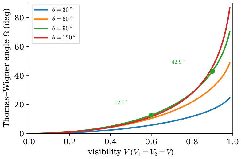
For two orthogonal measurements ($\theta ={90}^{\circ }$) with equal visibility $V_1=V_2=0.6$ (i.e., ${\xi }_1={\xi }_2=\mathrm{arctanh}\left(0.6\right)\approx 0.693$), $tanh(\xi /2)=tanh\left(0.347\right)\approx 0.333$, giving $tan(\mathsf{\Omega }/2)={0.333}^2\approx 0.111$, and hence $\mathsf{\Omega }\approx {12.7}^{\circ }$. For $V=0.9$: $\xi \approx 1.472$, $tanh(\xi /2)\approx 0.627$, giving $tan(\mathsf{\Omega }/2)\approx 0.393$, and hence $\mathsf{\Omega }\approx {42.9}^{\circ }$. The rotation grows nonlinearly with visibility, vanishes at $V=0$, and approaches $\theta$ as $V\to 1$ (pure-state limit). The deviation from the Pancharatnam prediction at the intermediate V is the measurable Beltrami–Klein signature.

• Concrete Protocol

Let us prepare a qubit in a mixed state ${\rho }_0$ with a Bloch vector of a magnitude r (purity parameter). We then perform partial measurements along $\widehat{z}$ and then $\widehat{x}$. We then reconstruct the final state via quantum state tomography. The acquired geometric rotation depends on the initial purity r according to the hyperbolic (Wigner) formula and not the spherical (Pancharatnam) formula, which applies only at $r=1$. This is achievable on superconducting qubit platforms with dispersive readout (measurement efficiency $\eta >0.5$, tomographic precision ∼$1\%$, ∼${10}^4$ shots per setting).

• Robustness to Decoherence

The rotation is set by the visibility V at each measurement. Thus, dephasing between and during the two partial measurements reduces V, and hence $\mathsf{\Omega }$, shifting the outcome toward the lower-visibility rows of

Table 3. Thomas–Wigner rotation $\mathsf{\Omega }$ from Equation (10) for equal visibilities $V_1=V_2=V$ and inter-axis angle $\theta$. Values in degrees.

$\mathit{\theta }\setminus \mathit{V}$	$0.30$	$0.60$	$0.90$	$0.95$
${30}^{\circ }$	$1.32$	$5.80$	$16.68$	$20.43$
${60}^{\circ }$	$2.31$	$10.42$	$31.75$	$39.56$
${90}^{\circ }$	$2.70$	$12.68$	$42.90$	$55.32$
${120}^{\circ }$	$2.37$	$11.64$	$45.90$	$63.19$

. The requirement is a separation of timescales; the total protocol duration ${\tau }_{\mathrm{tot}}$ (two partial measurements plus readout and reset) must satisfy ${\tau }_{\mathrm{tot}}\ll T_2$ so that the Bloch vector magnitude does not decay before tomography. For transmons with $T_2$∼$100 \mathsf{\mu }$s and dispersive readout of $0.1$–$1 \mathsf{\mu }$s, the sequence fits comfortably inside the coherence window. Because $\mathsf{\Omega }$ depends only on the instantaneous V, residual dephasing shifts the measured angle in a calculable way rather than erasing it; intermediate visibilities $V\approx 0.6$–$0.9$ are the recommended operating range.

The same dependence is plotted continuously in Figure 3, which shows how the acquired rotation grows with visibility at each inter-axis angle.

10.4. Consistency Check: ${\gamma }^2$ Scaling of Estimation Precision

Sweeping V and fitting $I\left(V\right)=a/{(1-V^2)}^b$ should return $b=1$ and $a=1$. We stress that this coincides with the prediction of standard Bernoulli estimation and therefore does not by itself distinguish the geometric interpretation from conventional quantum estimation; it is a consistency check and not a discriminating test. The genuinely discriminating prediction of this paper is the purity-dependent Thomas–Wigner rotation of Section 10.3, whose value at intermediate visibility (for example, $\mathsf{\Omega }={12.68}^{\circ }$ at $V=0.6$, $\theta ={90}^{\circ }$ and $\mathsf{\Omega }={42.90}^{\circ }$ at $V=0.9$) deviates from the pure-state Pancharatnam baseline $\mathsf{\Omega }\to \theta$ and is not reproduced by the naive $r=1$ treatment. A measured $b\ne 1$ would nonetheless falsify the underlying Fisher-information identity.

11. Status of Claims

Table 4. Claim status in this paper.

Claim	Basis	Status Here
$I\left(V\right)={\gamma }^2\left(V\right)$ (classical)	Direct computation, Section 2	Derived here
$F_Q\left(r\right)={\gamma }^2\left(r\right)$ (qubit radial QFI)	Standard qubit QFI/Bures formulas	Recalled (cited)
$d{s}_{\mathrm{BK}}^2=4{\gamma }^2\left(r\right) d{s}_{\mathrm{Bures}}^2$	Theorem 1	Derived here
Chentsov forces Fisher–Rao form in V	Proposition 1	Derived here
Bures or SLD is a distinguished monotone metric	Petz classification	Prior work (cited)
Measurement backaction generates boosts	Burns–Greenfield–Dressel	Prior work (cited)
Thomas–Wigner rotation for non-collinear updates	Cartan or boost composition + measurement model	Testable prediction
Conformal non-equivalence for $N\ge 3$	Theorem 2	Derived here
Gudermannian bridge $arcsin\left(V\right)=\mathrm{gd}(\mathrm{arctanh} V)$	Elementary identity, Section 5.4	Derived here

records the status of every claim made in this paper, separating results derived here from results recalled from the prior literature and from the single testable prediction.

12. Discussion

The identity $I\left(V\right)={\gamma }^2\left(V\right)$ is algebraically elementary. Its significance comes from four sources: Chentsov uniqueness at the classical level, the Petz classification at the quantum level (jointly establishing that ${\gamma }^2$ is the unique operationally optimal metric coefficient, up to normalization), the $\mathrm{SL}(2,\mathbb{C})\cong {\mathrm{Spin}}^{+}(1,3)$ group structure that provides the physical bridge to Lorentz kinematics, and consistency tests on existing qubit platforms.

• Completing Chen–Ungar

Chen and Ungar [1,2,3,4] identified the Bloch ball as a Beltrami–Klein model of hyperbolic geometry. This paper extends their algebraic identification to the metric level; the conformal equivalence Equation (7) quantifies the precise relationship between the two natural geometries of the Bloch ball, with the conformal factor equal to ${\gamma }^2$ and the identity between the Fisher information and the squared Lorentz factor. Han, Kim, and Noz [13,38] proved the group theory for squeezing (1988).Lévay [39] identified a connection between Thomas–Wigner rotation and Uhlmann parallel transport for qubits (2004); the present paper reframes this in terms of operationally accessible sequential measurements parametrized by visibility, yielding concrete numerical predictions (Equation (10)). Burns, Greenfield, and Dressel [10] proved the measurement dynamics (2026). The present paper provides the scalar identity and conformal equivalence linking these facets.

• Experimental Outlook

Recent experiments have brought the quantum geometric tensor and Fisher information into the laboratory. Zhao et al. [40] verified QFI–coherence factorization experimentally for qubit and qutrit systems. Sala et al. [41] reported direct measurement of the quantum metric in materials via spin-momentum-locked electrons. The ${\gamma }^2$ divergence as the band gap closes ($V\to 1$) is a testable prediction. Melo et al. [42] introduced conditional quantum Fisher information at the trajectory level. Oancea et al. [43] generalized the quantum geometric tensor using sub-bundle geometry.

13. Conclusions

We have shown that Fisher information of a binary quantum measurement equals the squared Lorentz factor: $I\left(V\right)={\gamma }^2\left(V\right)$ (Equation (1)). We proved that this identity reflects a conformal equivalence between the two natural geometries of the Bloch ball: $d{s}_{\mathrm{BK}}^2=4{\gamma }^2·d{s}_{\mathrm{Bures}}^2$ (Theorem 1). We established that this structure is algebraically special to qubits; the Weyl tensor of the Bures metric is non-vanishing for $N\ge 3$, providing a curvature obstruction to conformal equivalence with any constant-curvature model (Theorem 2). We identified the Thomas–Wigner rotation (Equation (10)) as a testable prediction for sequential non-collinear measurements.

These results complete the identification of the Bloch ball with the Beltrami–Klein model of hyperbolic geometry initiated by Chen and Ungar [1]. The conformal factor ${\gamma }^2=I\left(V\right)$ is the specific scalar relating their algebraic observation to the information-geometric structure of quantum measurement. That the same ${\gamma }^2$ and $\mathrm{SL}(2,\mathbb{C})$/Lorentz structure appears in polarization optics and in two-band condensed-matter systems for genuine two-level or two-mode states indicates that the identity is more than a formal coincidence while remaining an elementary statement about qubit geometry. The underlying framework was peer-reviewed in a companion paper on quantum-computing applications [44].

References

1. Chen, J.-L.; Ungar, A.A. The Bloch gyrovector. Found. Phys. 2002, 32, 531–565. [Google Scholar] [CrossRef] [Scilit]
2. Chen, J.-L.; Ungar, A.A. From the group SL(2, C ) to gyrogroups and gyrovector spaces and hyperbolic geometry. Found. Phys. 2001, 31, 1611–1639. [Google Scholar] [CrossRef] [Scilit]
3. Chen, J.-L.; Ungar, A.A. Introducing the Einstein metric to quantum computation and quantum information geometry. Found. Phys. Lett. 2002, 15, 189–197. [Google Scholar] [CrossRef] [Scilit]
4. Ungar, A.A. Gyrovector spaces and their differential geometry. Nonlinear Funct. Anal. Appl. 2008, 13, 295–323. [Google Scholar]
5. Alsing, P.M.; Cafaro, C.; Felice, D.; Luongo, O. Geometric aspects of mixed quantum states inside the Bloch sphere. Quantum Rep. 2024, 6, 90–109. [Google Scholar] [CrossRef] [Scilit]
6. Penrose, R.; Rindler, W. Spinors and Space-Time; Cambridge University Press: Cambridge, UK, 1984; Volume 1. [Google Scholar]
7. Wootters, W.K. Statistical distance and Hilbert space. Phys. Rev. D 1981, 23, 357–362. [Google Scholar] [CrossRef] [Scilit]
8. Chen, J.-L.; Fu, L.; Ungar, A.A.; Zhao, X.-G. Geometric observation for Bures fidelity between two states of a qubit. Phys. Rev. A 2002, 65, 024303. [Google Scholar] [CrossRef] [Scilit]
9. Petz, D. Monotone metrics on matrix spaces. Lin. Alg. Appl. 1996, 244, 81–96. [Google Scholar] [CrossRef] [Scilit]
10. Burns, L.; Greenfield, S.; Dressel, J. Delayed choice Lorentz transformations on a qubit. Quantum Stud. Math. Found. 2026, 13, 10. [Google Scholar] [CrossRef] [Scilit]
11. Pires, D.P.; Cianciaruso, M.; Céleri, L.C.; Adesso, G.; Soares-Pinto, D.O. Generalized geometric quantum speed limits. Phys. Rev. X 2016, 6, 021031. [Google Scholar] [CrossRef] [Scilit]
12. Taddei, M.M.; Escher, B.M.; Davidovich, L.; de Matos Filho, R.L. Quantum speed limit for physical processes. Phys. Rev. Lett. 2013, 110, 050402. [Google Scholar] [CrossRef] [Scilit] [PubMed]
13. Han, D.; Kim, Y.S.; Noz, M.E. Linear canonical transformations of coherent and squeezed states in the Wigner phase space. Phys. Rev. A 1988, 37, 807–814. [Google Scholar] [CrossRef] [Scilit]
14. Yurke, B.; McCall, S.L.; Klauder, J.R. SU(2) and SU(1, 1) interferometers. Phys. Rev. A 1986, 33, 4033–4054. [Google Scholar] [CrossRef] [Scilit]
15. Tse, M.; Yu, H.; Kijbunchoo, N.; Fernandez-Galiana, A.; Dupej, P.; Barsotti, L.; Blair, C.; Brown, D.; Dwyer, S.; Effler, A.; et al. Quantum-enhanced advanced LIGO detectors in the era of gravitational-wave astronomy. Phys. Rev. Lett. 2019, 123, 231107. [Google Scholar] [CrossRef] [Scilit] [PubMed]
16. Zanardi, P.; Giorda, P.; Cozzini, M. Information-theoretic differential geometry of quantum phase transitions. Phys. Rev. Lett. 2007, 99, 100603. [Google Scholar] [CrossRef] [Scilit] [PubMed]
17. Peres, A.; Scudo, P.F.; Terno, D.R. Quantum entropy and special relativity. Phys. Rev. Lett. 2002, 88, 230402. [Google Scholar] [CrossRef] [Scilit] [PubMed]
18. Giacomini, F.; Castro-Ruiz, E.; Brukner, Č. Quantum mechanics and the covariance of physical laws in quantum reference frames. Nat. Commun. 2019, 10, 494. [Google Scholar] [CrossRef] [Scilit] [PubMed]
19. Giacomini, F.; Castro-Ruiz, E.; Brukner, Č. Relativistic quantum reference frames: The operational meaning of spin. Phys. Rev. Lett. 2019, 123, 090404. [Google Scholar] [CrossRef] [Scilit] [PubMed]
20. Apadula, L.; Castro-Ruiz, E.; Brukner, Č. Quantum reference frames for Lorentz symmetry. Quantum 2024, 8, 1440. [Google Scholar] [CrossRef] [Scilit]
21. Palge, V.; Dunningham, J.A. Relativistic quantum information and time machines. Ann. Phys. 2015, 363, 275–304. [Google Scholar] [CrossRef] [Scilit]
22. Wilde, M.M. Quantum Information Theory; Cambridge University Press: Cambridge, UK, 2013. [Google Scholar]
23. Wootters, W.K. Entanglement of formation of an arbitrary state of two qubits. Phys. Rev. Lett. 1998, 80, 2245–2248. [Google Scholar] [CrossRef] [Scilit]
24. Mintert, F.; Buchleitner, A. Observable entanglement measure for mixed quantum states. Phys. Rev. Lett. 2007, 98, 140505. [Google Scholar] [CrossRef] [Scilit] [PubMed]
25. Berta, M.; Christandl, M.; Colbeck, R.; Renes, J.M.; Renner, R. The uncertainty principle in the presence of quantum memory. Nat. Phys. 2010, 6, 659–662. [Google Scholar] [CrossRef] [Scilit]
26. Adlam, E.; Rovelli, C. Information is physical: Cross-perspective links in relational quantum mechanics. Philos. Phys. 2023, 1, 4. [Google Scholar] [CrossRef] [Scilit]
27. Di Biagio, A.; Rovelli, C. Relative information, relative facts. arXiv 2025, arXiv:2510.11349. [Google Scholar]
28. Perche, T.R.; Martín-Martínez, E. Geometry of spacetime from quantum measurements. Phys. Rev. D 2022, 105, 066011. [Google Scholar] [CrossRef] [Scilit]
29. Besse, A.L. Einstein Manifolds; Springer: Berlin/Heidelberg, Germany, 1987. [Google Scholar]
30. Dittmann, J. Some properties of the Riemannian Bures metric on mixed states. J. Geom. Phys. 1994, 13, 203–206. [Google Scholar] [CrossRef] [Scilit]
31. Dittmann, J. On the Riemannian metric on the space of density matrices. Rep. Math. Phys. 1995, 36, 309–315. [Google Scholar] [CrossRef] [Scilit]
32. O’Neill, B. The fundamental equations of a submersion. Mich. Math. J. 1966, 13, 459–469. [Google Scholar] [CrossRef] [Scilit]
33. Uhlmann, A. The metric of Bures and the geometric phase. In Groups and Related Topics; Springer: Dordrecht, The Netherlands, 1992; pp. 267–274. [Google Scholar]
34. Kang, M.; Kim, S.; Qian, Y.; Neves, P.M.; Ye, L.; Jung, J.; Puntel, D.; Mazzola, F.; Fang, S.; Jozwiak, C.; et al. Measurements of the quantum geometric tensor in solids. Nat. Phys. 2025, 21, 110–117. [Google Scholar]
35. Kim, S.; Chung, Y.; Qian, Y.; Park, S.; Jozwiak, C.; Rotenberg, E.; Bostwick, A.; Kim, K.S.; Yang, B.-J. Direct measurement of the quantum metric tensor in solids. Science 2025, 388, 1050–1054. [Google Scholar] [CrossRef] [Scilit] [PubMed]
36. Rhodes, J.A.; Semon, M.D. Relativistic velocity space, Wigner rotation, and Thomas precession. Am. J. Phys. 2004, 72, 943–960. [Google Scholar] [CrossRef] [Scilit]
37. Yeh, L. Wigner rotation and Euler angle parametrization. Am. J. Phys. 2023, 91, 547–556. [Google Scholar] [CrossRef] [Scilit]
38. Baskal, S.; Kim, Y.S.; Noz, M.E. Physics of the Lorentz Group, 2nd ed.; IOP Publishing: Bristol, UK, 2021. [Google Scholar]
39. Lévay, P. Thomas rotation and the mixed state geometric phase. J. Phys. A Math. Gen. 2004, 37, 4593–4605. [Google Scholar] [CrossRef] [Scilit]
40. Zhao, X.; Yu, X.; Li, L.; Zhou, W.; Zhang, C. Factorization dynamics between quantum Fisher information and quantum coherence. Sci. Adv. 2025, 11, eadv8132. [Google Scholar] [CrossRef] [Scilit] [PubMed]
41. Sala, G.; Mercaldo, M.T.; Domi, K.; Gariglio, S.; Cuoco, M.; Ortix, C.; Caviglia, A.D. The quantum metric of electrons with spin-momentum locking. Science 2025, 389, 822–825. [Google Scholar] [CrossRef] [Scilit] [PubMed]
42. Melo, P.B.; Paraguassú, P.V.; Queirós, S.M.D.; Iemini, F.; Paternostro, M.; Morgado, W.A.M. Stochastic quantum information geometry and speed limits at the trajectory level. arXiv 2026, arXiv:2601.12475. [Google Scholar]
43. Oancea, M.A.; Mieling, T.B.; Palumbo, G. Quantum geometric tensors from sub-bundle geometry. Quantum 2026, 10, 1965. [Google Scholar] [CrossRef] [Scilit]
44. Srivats, B.G. The squared Lorentz factor in quantum computation: Grover search, quantum batteries, and the Zeno effect. Next Res. 2026, 10, 101888. [Google Scholar] [CrossRef] [Scilit]
Figure 1. Distance from the center of the Bloch ball to visibility V. The spherical Fisher–Rao distances (QFI: arcsin V π / 2 ; Bures: 1 2 arcsin V π / 4 ) remain finite as V 1 , while the hyperbolic Beltrami–Klein distance artanh   V diverges. The divergence is a property of the hyperbolic coordinate model and not a physical barrier on state transitions.
Quantumrep 08 00068 g001
Figure 2. Bures sectional curvature at the maximally mixed state ρ * = I / N (Bures-orthonormal units). For N = 2 , every plane gives K B = 4 (constant). For N = 3 , the Cartan (commuting) plane gives K B = 1 , and the root (non-commuting) plane gives K B = 11 / 2 . Thus, the curvature is non-constant, and the Weyl tensor cannot vanish (Appendix A).
Quantumrep 08 00068 g002
Figure 3. Purity-dependent Thomas–Wigner angle Ω ( V ) from Equation (10) for several inter-axis angles θ , with V 1 = V 2 = V . The rotation vanishes at V = 0 and approaches θ as V 1 ; the deviation from the pure-state (Pancharatnam) baseline at intermediate V is the measurable signature.
Quantumrep 08 00068 g003