Article

QGeo: A Python Package for Calculating Geodesic Control Functions for Quantum Computing

1
Naval Information Warfare Center Pacific, San Diego, CA 92152, USA
2
U.S. Naval Research Laboratory, Washington, DC 20375, USA
3
Mathematics Department, San Diego State University, San Diego, CA 92152, USA
*
Author to whom correspondence should be addressed.
Quantum Rep. 2026, 8(2), 30; https://doi.org/10.3390/quantum8020030
Submission received: 2 February 2026 / Revised: 24 March 2026 / Accepted: 27 March 2026 / Published: 1 April 2026

Abstract

We present a new Python package that uses the formalism of geometric quantum complexity to numerically compute metric-dependent geometric cost and control functions associated with preparing a given unitary transformation on a quantum computer. The numerical procedure we implement is presented and discussed. Analyzed quantum circuits include: the quantum Fourier transform for up to four qubits, a random circuit with depth 100, and a circuit for analyzing the evolution of a fermionic chain with several lattice sites.

1. Introduction

Quantum computers implement unitary transformations on quantum states. In practice, this is done by decomposing a target unitary transformation into a product of elementary unitary transformations called quantum gates such that the target unitary transformation can be expressed as
U T = g N g 1 .
Here the g i s are elementary quantum gates. The set of available elementary gates depends on the specific quantum computer being used. At the hardware level, the implementation of these gates is specialized (for example implementations of elementary gates on superconducting qubits, see [1]), and most mainstream platforms for quantum computation usually have a relatively small set of elementary gates available. For example, the IBM quantum computer Torino can only implement tensor products of: the identity matrix, an X gate, an SX gate, an Rz gate, and a controlled-Z gate [2].
The number of gates required to implement a target unitary is called the gate complexity [3]. Given an elementary gate set, a quantum processor, and a target unitary transformation, the problem of finding an implementation of the target unitary that minimizes the complexity is called the quantum circuit mapping problem, which is known to be difficult [4].
An alternative measure of complexity for a unitary operator is the geodesic quantum complexity [5]. In this approach, the difficulty is associated with preparing a given unitary matrix specified by a metric on the unitary group and then looking for curves of minimal length that connect the identity operator to the target unitary matrix. These minimal length curves are called geodesics and the length of the minimal geodesic is a measure of complexity. This contrasts with other optimal control methods such as the [6] Krotov that optimizes for fidelity in the presence of noise and restricted control sets.
Concretely, the evolution of the quantum state is generated by a Hamiltonian H ( t ) . This implies a unitary evolution that is given by
U ( t ) = T e i 0 t d t H ( t ) ,
T is the time-ordering operator, which orders operators in descending time order such that operators evaluated at the latest times are on the left. In (A2) it is shown that this is a solution to the Schrödinger equation.
Onto (2) we impose the boundary conditions: U ( 0 ) = I and U ( T ) = U T . This evolution defines a path γ , in the unitary group, and the length of that path is specified by a phenomenologically motivated real-valued, symmetric, inner product defined by
H , J = 1 2 n tr H G ( J ) ,
where J is another Hamiltonian operator, n is the number of qubits and the map G is a super-operator defined in Equation (6) that penalizes operations that have weight greater than two. This is a highly idealized proxy for conditions where the implementation of three- or more-qubit gates is difficult. The length of the path is given by (4). The length of the path that minimizes (4) is interpreted as the complexity of the target unitary, with respect to this metric.
C [ γ ] = 0 T H ( t ) , H ( t ) 1 / 2 d t .
Paths on which this complexity is stationary are called geodesics. While geodesic paths may not be global minima of the complexity, the global minimum will correspond to a geodesic path. Since its inception, geodesic complexity has been applied across multiple areas, including quantum information and quantum gravity [3,7,8,9,10,11,12,13].
Part of the original motivation for formulating the notion of geodesic quantum complexity was to put lower bounds on the exact gate complexity, and an upper bound on the approximate gate complexity associated with preparing U. To our knowledge, however, it has not been applied to its original purpose of bounding gate complexities of operationally relevant unitary matrices. The purpose of this article it to apply the formalism of geometric complexity to several examples, including the quantum Fourier transform. In Section 2, the problem is defined more concretely and strategy for solving it is discussed. In Section 3, analytic approximations to the problem are discussed. The numerical implementation of the strategy and specific calculations of geodesic complexities are then presented in Section 4.

2. Approach

In this section, we discuss a numerical approach for calculating the geodesic quantum complexity of a given unitary operator, and a particular metric. Essentially, our problem consists of calculating solutions of the Schrödinger-geodesic equation, which is a coupled set of ordinary differential equations that are discussed below. Our solutions are subject to the boundary conditions U ( 0 ) = I , and U ( T ) = U T . This is a boundary value problem. A standard tool for numerically solving this kind of problem is shooting [14]. However, because the dimensionality of our problem is very high, shooting is no longer effective and other approaches must be used. We approach this problem as in [15]. To keep this report self-contained we reproduce details of this method here.
The Schrödinger-geodesic equation is derived by Dowling and Nielsen [15] and is given by:
U ˙ t + i H t U t = 0 , H ˙ + i F H , G H = 0 ,
Again, subject to the boundary conditions: U ( 0 ) = I , and U ( T ) = U T . The solutions of this system of equations will be curves on S U 2 n . Moreover, solving this system give us the tangent vectors/Hamiltonian H that can then be used in (4) to calculate the complexity of this path. The super-operator G , and its inverse super-operator F are:
G = P + q Q , F = P + q 1 Q .
P is the identity map on generators of one- and two-qubit operations and the zero map on generators of three- and higher-qubit operations. The map Q is the zero map on one and two qubit operations, and the identity map on three and higher qubit operations. The parameter q is a factor that penalizes operations corresponding to more than two qubits. This is to mimic conditions where operations spanning more than two qubits must be synthesized from two-qubit gates. It is therefore useful for studying algorithms that must be phrased in terms of gates with two or fewer gates from a geometric perspective. q = 4 n is a regime of computational interest, which was used in the original iteration of this algorithm because it was observed that complexities and initial values of control functions converged [15].
We set the initial condition in Equation (5) to be H 0 = V 0 i σ i , where V 0 i are real constants, and i σ i is a basis for su 2 n . The σ i are constructed from taking n 1 Kronecker products of the Pauli matrices in su 2 .

Solution Strategy

Having stated the problem, we discuss the strategy for constructing a solution to the boundary value problem specified at (5). Given a solution to the problem for a given penalty factor, q, it is possible to construct the solution for, q + Δ when Δ is small enough. This is because for this regime, the problem can be linearized, and then analyzed more easily. Using this perturbative approach, a solution to (5) can be constructed for arbitrarily large penalty factor, including the regime where q 4 n . The base case for this procedure is the q = 1 case. As will be discussed later, this case can be solved analytically, and therefore serves as a good starting point. Given a solution to (5) for a given q, U q ( t ) , we model the solution at q + Δ as:
U q + Δ = U q ( t ) e i Δ J ( t ) .
This implies a perturbation to the Hamiltonian that can be found by computing the quantity: i U ˙ U . This is found to be
i U ˙ U = H q + Δ = H q + Δ U q ( t ) J ˙ ( t ) U q ( t ) + O ( Δ 2 ) = H q + Δ K ( t ) + O ( Δ 2 ) .
where we have defined K ( t ) = U q ( t ) J ˙ ( t ) U q ( t ) . To constrain that H q + Δ is still a solution to the geodesic equation, we plug it into (5), and expand to first order in Δ . To first order in Δ , we find the constraint on K:
0 = K ˙ + i F ( K , G ( H q ) + H q , G ( K ) + Q ( F ( G ( H q ) , H q ) ) + H q , Q ( H q ) ) = K ˙ + i F K , G ( H q ) + H q , G ( K ) + i F 2 P ( H q ) , Q ( H q ) .
We used the fact that P Q = 0 , P 2 = P , Q 2 = Q . This is the so called “lifted” Jacobi equation. It is an inhomogeneous linear system, and so its general solution can be written as:
K ( t ) = K t ( K ( 0 ) ) K t 0 t d τ K t 1 ( C ( τ ) ) .
where K t is a linear operator, which propagates the initial value of K ( 0 ) such that it solves the homogeneous part of the (9), and C = i F 2 P ( H q ) , Q ( H q ) is the inhomogeneous part of (9). By expressing this equation in terms of coordinates, it turns out to be possible to derive an expression for K t . Expressing the homogeneous part of (9), in terms of coordinates we find:
0 = K ˙ i j + i F i j k l ( K k α G α l β δ H β δ ( q ) G k α β δ H β δ ( q ) K α l + H k α ( q ) G α l β δ K β δ G k α β δ K β δ H α l ( q ) ) = K ˙ i j + i F i j k l ( δ k β G δ l γ ϵ H γ ϵ ( q ) G k β γ ϵ H γ ϵ ( q ) δ δ l + H k α ( q ) G α l β δ G k α β δ H α l ( q ) ) K β δ = K ˙ i j i A i j β δ K β δ .
Here we are using Einstein summation notation, and we have defined the tensor:
A i j β δ = F i j k l δ k β G δ l γ ϵ H γ ϵ ( q ) G k β γ ϵ H γ ϵ ( q ) δ δ l + H k α ( q ) G α l β δ G k α β δ H α l ( q ) .
The homogeneous propagator can then be expressed as an ordered exponential:
K ( t ) i j k l = T e i 0 t d t A ( t ) i j k l ,
where we are suppressing indices inside of the time-ordering operator for notational convenience. We can think of this as a normal matrix equation where the first two indices of A correspond to the first index of a matrix and the last two indices of A correspond to the last index of a matrix. From this flattened perspective, A takes the form:
A = F [ ( I L L T I ) + ( H T I I H ) G ] .
Note that in the equation above, we have replaced super-operators F and G with their matrix representations,
F = 1 2 n β 1 g ( β ) σ β σ β , G = 1 2 n β g ( β ) σ β σ β , g ( β ) = 1 if β 2 , q else .
This matrix representation is an eigen-decomposition of the relevant super-operators. We require that the lifted Jacobi field has boundary conditions J ( 0 ) = J ( T ) = 0 , so the boundaries of the geodesic stay fixed. To accomplish this observe the relationship:
J ( T ) = 0 T d t J ˙ ( t ) = 0 T d t U K ( t ) U = 0 T d t U K t ( K ( 0 ) ) U 0 T d t U K t 0 t d τ K t 1 ( C ( τ ) ) U = J T J ˙ ( 0 ) 0 T d t U K t 0 t d τ K t 1 ( C ( τ ) ) U .
where we have identified J ˙ ( 0 ) = K ( 0 ) . J ( 0 ) is set to zero here as an initial condition for K. Because we need J ( T ) = 0 , we set it to zero in the above equation, and solve for J ˙ ( 0 ) . The result is:
J ˙ ( 0 ) = J T 1 0 T d t U K t 0 t d τ K t 1 ( C ( τ ) ) U .
This gives us a way to update our initial Hamiltonian from q to q + Δ because according to (8):
J ˙ ( 0 ) = H q ( 0 ) q H q + Δ ( 0 ) H q ( 0 ) Δ .
The right-hand side (RHS) of (16) simplifies and finally, a calculation shows:
d H q ( 0 ) d q = J T 1 ( 0 T d t U ( t ) i t [ P ( H ) , Q ( H ) ] U ( t ) ) , q = 1 , ( J T 1 ( L ( 0 ) ) T L ( 0 ) ) / q ( q 1 ) , q > 1 ,
where L ( 0 ) = G ( H ( 0 ) ) . The base case for this update rule is given when q = 1 . In this case it is especially easy to calculate solutions to (5) because the metric and its inverse are identity operators on the Lie algebra. Concretely for this case we have:
U ˙ t + i H t U t = 0 H ˙ = 0 ,
which is still subject to the boundary condition: U ( 0 ) = I , and U ( T ) = U T . In this case, the Hamiltonian is a constant and its initial value is given by H 1 ( 0 ) = i T log U T . A derivation of this solution will be presented in the analytical section. Given this initial Hamiltonian and the update rule given at (18) it is possible to construct solutions that hit the target unitary for arbitrarily large penalty factors.

3. Analytic Approximations

In this section, we consider analytic solutions and approximations to our problem. Analytic solutions and approximations give context for our full numerical solutions. In the 1- and 2-qubit cases, su 2 and su 4 , the geodesic equation simplifies to H ^ ˙ = 0 because G is the identity operator on traceless 2-qubit operations. This gives us analytic values on the complexities that we can then compare to our numerical solutions.
When H ^ ˙ = 0 , we have the solution on the interval 0 , T
U ( t ) = e i H ^ t I ,
where we are imposing the boundary conditions: U ( 0 ) = I , and U ( T ) = U T . The boundary condition at time T fixes the Hamiltonian in this case:
H ^ = i T log U T .
Here we are computing logarithms of matrices by first diagonalizing the matrix and taking the logarithm of the eigenvalues. Because U T is a unitary matrix, the eigenvalues are complex phases. When we take logarithms, we compute the phase such that they are on the principal branch, i.e., they take values between π , π . Any other branch choice introduces some spurious cost. To mitigate unitary drift, eigenvalues are normalized to have absolute value one, ensuring that small numerical errors in the eigenvalues do not affect the logarithm. This uniquely determines the Hamiltonian despite the ambiguity associated with the logarithm. From here, plugging into (3) and (4), we find the approximate complexity to be
C 1 2 n tr log U T G log U T .
This is the complexity associated with a straight line path from the identity operator to the target unitary. For one and two qubits it is an exact value of the complexity and for high numbers of qubits it serves as an approximation to which we can compare our exact answers.

3.1. One Qubit

In the case of one qubit, the Lie algebra is s u ( 2 ) , with three dimensions spanned by σ x , σ y and σ z . General elements in this algebra are given by H = V i σ i , and the inner product simplifies to:
H , J = 1 2 t r H G ( J ) = H i J j 1 2 t r ( σ i σ j ) = g i j H i J j .
where we have defined
g i j = 1 0 0 0 1 0 0 0 1 .
This is the normal inner product one uses on Euclidean space. In the following, we consider the target unitary matrix, which corresponds to the quantum Fourier transform on one qubit:
U T = i 2 1 1 1 1 .
To construct a geodesic that hits this target, we first compute the matrix logarithm to obtain the Hamiltonian. This is most easily done using computer algebra and the result is:
H = π 2 2 1 1 1 1 .
Now to obtain the geodesic connecting the identity and target, we need to solve the Shrödinger equation: U ˙ = i H U . Because the Hamiltonian is a constant here, this can be done using the matrix exponential: U = e i H t . Computing this quantity and simplifying, we find:
U t = α t β t β t β t α t + β t α t = cos π 2 t β t = i 2 sin π 2 t .
Finally, it is possible to compute the complexity. It is given by C = 1 2 t r ( H H ) = π 2 2 .

3.2. Two Qubits

In the case of two qubits, the Lie algebra we work with is s u ( 4 ) and it is spanned by Kronecker products of at most two Pauli matrices. This space is 15-dimensional and the different basis elements are shown in (A7), and because no three-qubit operations are allowed at this stage, the super-operator G is still an identity operation on traceless unitary matrices. Because of this, the metric tensor is given by:
g i j = δ i j .
where δ i j is the normal Kronecker delta, corresponding to a Euclidean inner product on this 15-dimensional space.
We consider now the following target unitary matrix, which corresponds to the two-qubit quantum Fourier transform:
U T = 1 2 n 1 1 1 1 1 ω ω 2 ω 3 1 ω 2 1 ω 2 1 ω 3 ω 2 1 .
where we have defined the variable:
ω = e π i / 2 .
As in the previous section, we then compute the Hamiltonian using matrix logarithms, and use that Hamiltonian in a matrix exponential to construct the geodesic path to the target unitary matrix. Up to a global phase, we find that path is given by:
U t = 1 4 ω 3 4 t α γ γ γ γ β δ ϵ γ δ α δ γ ϵ δ β , α = ω 2 t + 3 , β = 1 + ω t 2 , γ = 1 ω 2 t , δ = ω 2 t 1 , ϵ = ω t 1 2 .
Again, we can compute the complexity according to C = 1 4 t r ( H H ) = 11 π 16 .
For the gate set mentioned earlier: G = X , S x , R z ( θ ) , C z the complexities can be computed analytically and the results are:
C ( X ) = π 2 , C ( S x ) = π 4 , C ( R z ( θ ) ) = abs atan 2 sin ( θ ) , cos ( θ ) , C ( C Z ) = 3 π 4 .
These gate results will be used later on in order to create a point of comparison by transpiling circuits into the gate set G, and then the complexity of each gate is computed using these analytic formulas and summed. This is the gate-sum complexity and in Section 5 it is used to benchmark the geodesic compilation of full circuits.

3.3. Several Qubits

When we have more than two qubits, the solution to the geodesic equation is no longer a constant Hamiltonian; this makes the unitary evolution determined by Schrödinger’s Equation (19) much more difficult to calculate analytically. As a first approximation, in this section, we consider paths in the unitary group corresponding to constant Hamiltonians that hit the target. These paths are not geodesic and so do not minimize the complexity, but they do put upper bounds on the complexity that can be used to give our numerical solutions context. Here we call paths with a constant Hamiltonian simple.
Our procedure for doing this is the same as the two previous subsections. Starting with the target unitary matrix, we first compute the Hamiltonian using matrix logarithms. After that, the path in the unitary group is found by computing the Matrix exponential: U = e i H t . Finally, the complexity is computed according to the formula C H , H 1 / 2 . We have computed this simple-path complexity for the quantum Fourier transform for up to 10 qubits. The results are shown in the Figure 1, which also contains numerically computed geodesic complexities for up to four qubits and the corresponding gate-sum complexities.

4. Numerical Analysis

In this section we discuss the details associated with creating a numerical program that can compute quantum computational geodesics.
To make unitary matrices that correspond to quantum circuits we use a package in qiskit that has built-in functionality to do this. For example, constructing the N-qubit quantum Fourier transform matrix representation can be accomplished with the commands:
Quantumrep 08 00030 i001
This procedure is quite general and can be used to construct the matrix representation of any qiskit circuit object. Once the target unitary operator has been obtained we then compute the Hamiltonian H 0 for the desired unitary at time T = 1 in the case where q = 1 , taking a matrix logarithm as suggested by (A3). To compute matrix logarithms, we developed our own code to have tighter controls over ambiguities associated with logarithms. In this way, we compute logarithms using the code:
Quantumrep 08 00030 i002
This logarithm works by first diagonalizing the unitary matrix and then taking the log of the eigenvalues such that they are on the principal branch, i.e., they take values between π , π . The basis is then changed to the original one and the log of the matrix is returned.
Generally, all functions we use are decorated with the @njit operator such that functions are precompiled and run much faster at runtime.
Because we are only considering target unitaries that can be generated by elements of the Lie algebra s u ( 2 n ) , we substract the zero-point energy of the Hamiltonian. This amounts to a constant shift of the energy levels of the Hamiltonian, which does not affect its dynamics. This is accomplished by: H = H 0 1 2 n t r ( H 0 ) I , where H 0 is specified according to (21) and the complex unitary log function specified earlier is used. This effectively makes the Hamiltonian traceless. Generally, we remove global phases of circuits because they are not observables. Using the chosen metric, the cost of a global phase is not defined.
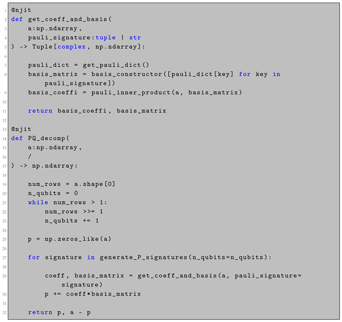
At this stage we need to compute the RHS of (18). To begin we develop a numerical implementation of the super-operators: F and, G . This can be done by implementing the super-operators P , and Q numerically. Generally, the operators P and Q operate on objects of the form V i σ i , where V i are real coefficients and σ i is a Pauli string. For three qubits, all Pauli strings are shown in (A8). From there the coefficient can be obtained from V i = 1 2 n t r ( V j σ j σ i ) , one can then count the number of Pauli matrices in a given Pauli string, which is associated with V i . This is the weight of the Pauli string. For example, P ( V i σ i ) = i w i V i σ i , where w i goes to zero if the weight is greater than 2 and one otherwise. In Python code this is implemented by:
Quantumrep 08 00030 i003
Once the super-operators P , and Q have been implemented we need to solve for the time evolution of the Hamiltonian and U ( t ) , essentially, numerically finding solutions to (5). We do this using the scipy.integrate.solve_ivp function with the “RK45” method. We solve over the range t 0 , 1 , and we record the solution value at N t linearly spaced points along this interval. These points will be used later on for computing the integrals in (18). During the solution however, solve_ivp may take as many steps as it needs to satisfy the default tolerance values for rtol and atol, which are 10 3 and 10 4 respectively. Besides the usual failure modes associated with solve_ivp, an extra condition has been implemented to check if the Jacobi propagator is well conditioned. If the condition number is above a threshold of 10 12 the solver exits and stops running.
Numerically now, we must calculate the Jacobi propagator. Again, this object is defined as
J T J ˙ ( 0 ) = 0 T d t U K t ( J ˙ ( 0 ) ) U .
Expressing this in terms of coordinates we find:
J T i j γ δ J ˙ γ δ ( 0 ) = 0 T d t U i α K t α β γ δ U β j J ˙ γ δ ( 0 ) .
The K propagator can be computed according to (13). We find it is most efficient to compute the ordered matrix exponential using a product:
K t α β γ δ = i = 1 i = t f e i Δ t i A ( t i ) .
where values for A are determined from our solutions for H, and U, which have been recorded on N t linearly spaced points on 0 , 1 . Numerically, we implement (35) directly as written. Concretely, A is calculated from (12). It is understood that operators evaluated at later times are placed towards the left. Putting all of this together, we then compute J T i j γ δ = 0 T d t U i α K t α β γ δ U β j . In Python, this can be done with one line:
Quantumrep 08 00030 i004
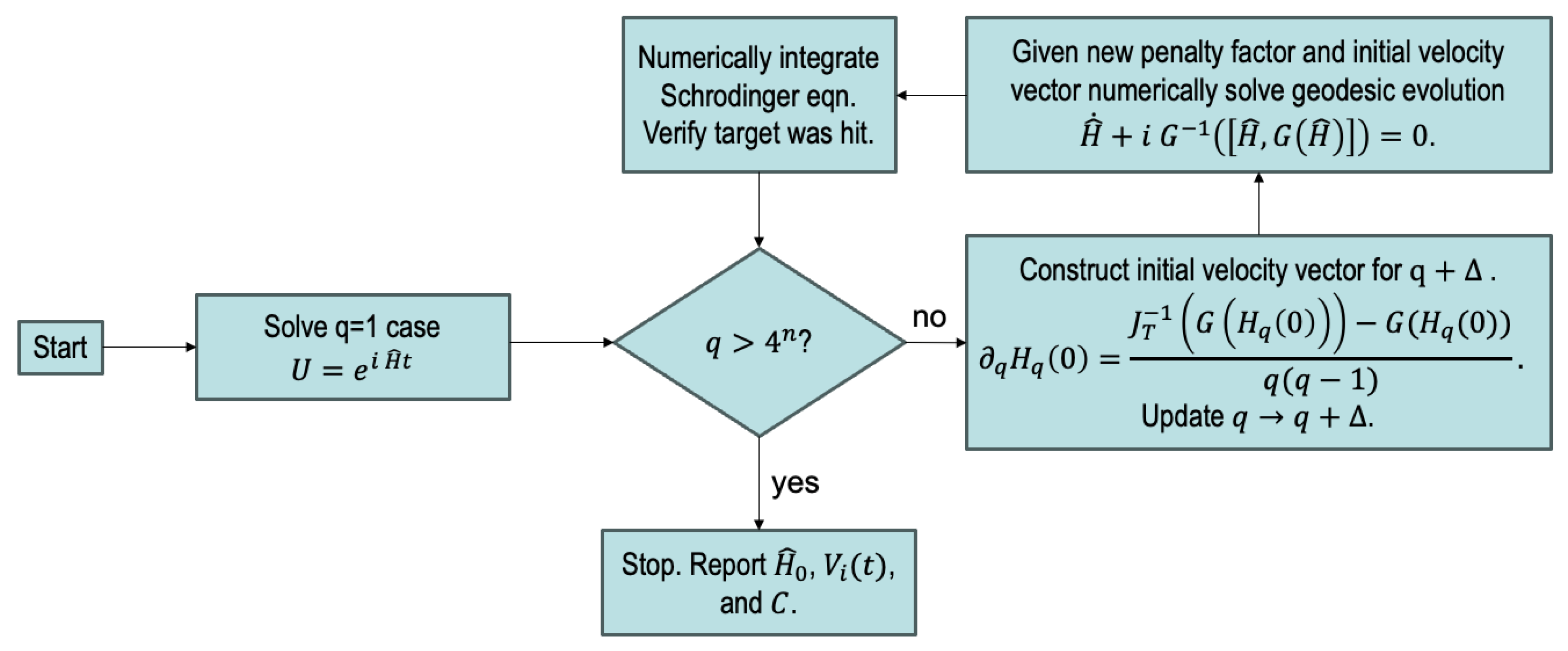
In all cases we numerically compute integrals with the trapezoid method. To obtain the inverse Jacobi propagator we reshape this tensor into a matrix and then invert it. Using this technique, we are able to evaluate (18) and we use solve_ivp to solve it as a differential equation. A flowchart summarizing the continuation scheme discussed above is shown in Figure A1.

4.1. Results

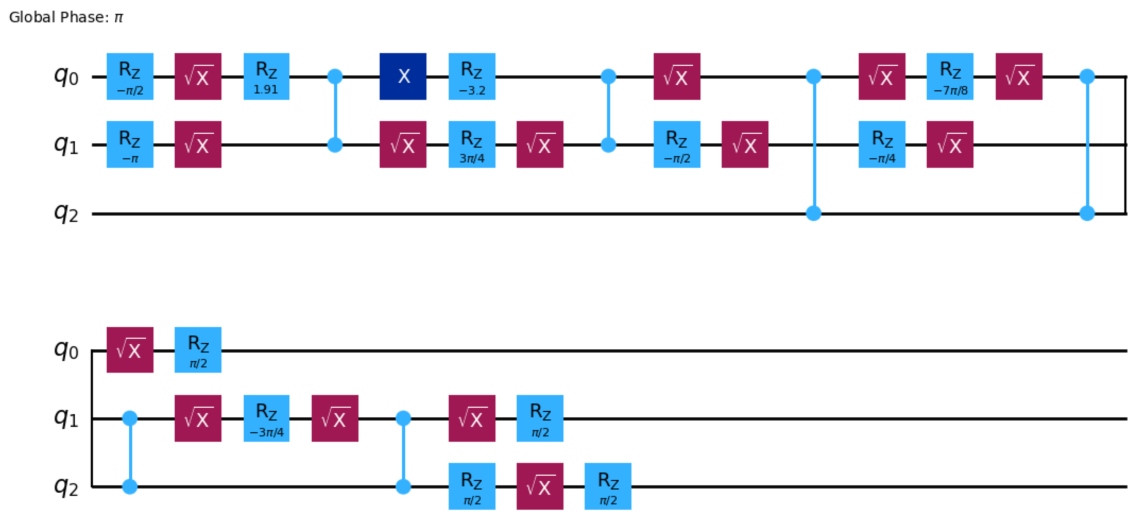
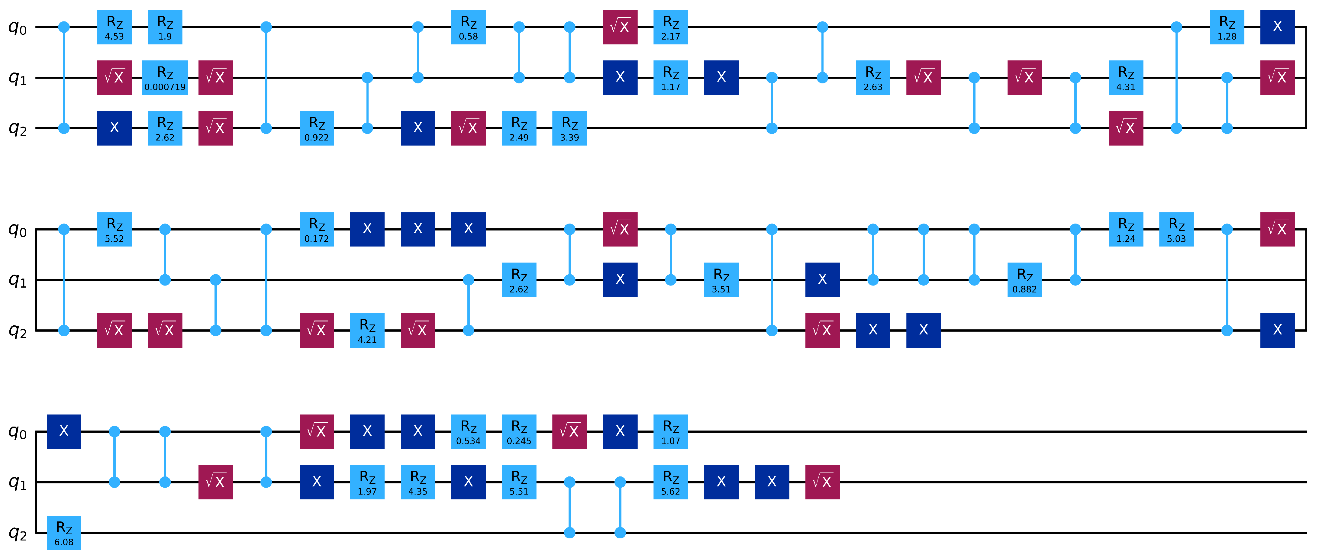
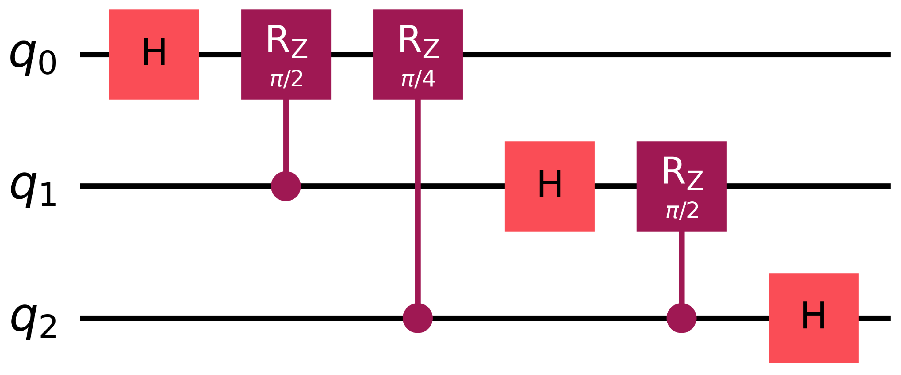
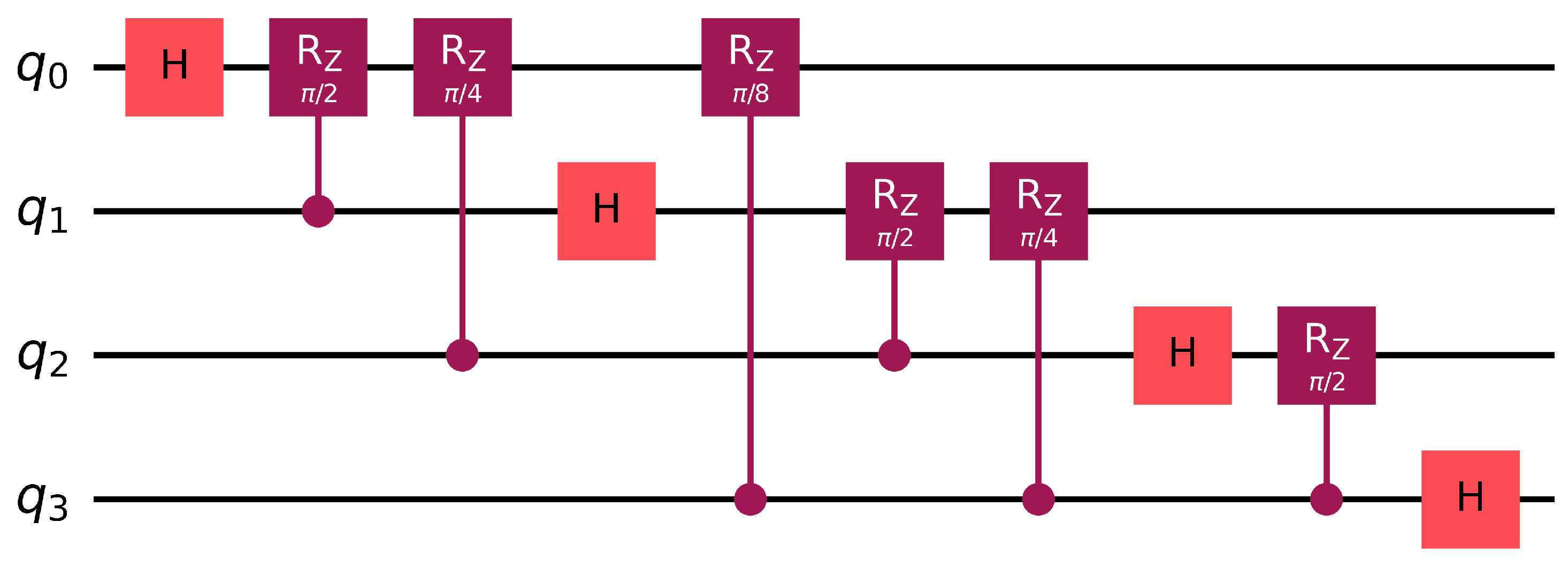
In this section we consider two numerical examples, and discuss our results. As a first numerical example, we consider the three- and four-qubit quantum Fourier transform. As a second example, we consider a randomly generated three-qubit quantum circuit with a depth of 100 gates. The randomly generated circuit can be seen in Figure A2. The three- and four-qubit quantum Fourier transform can be seen in Figure A3 and Figure A5.
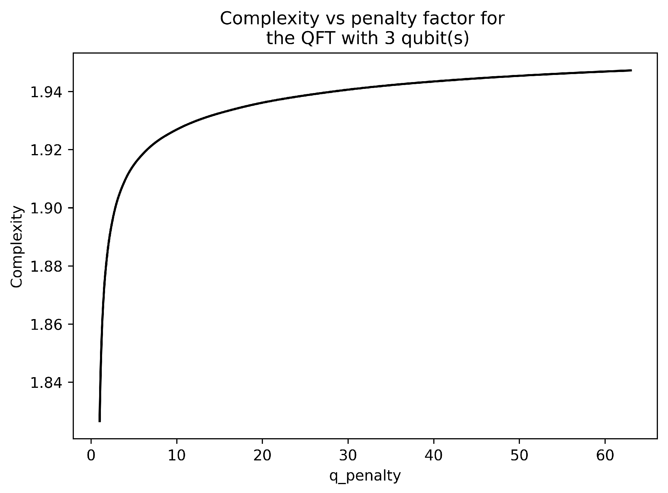
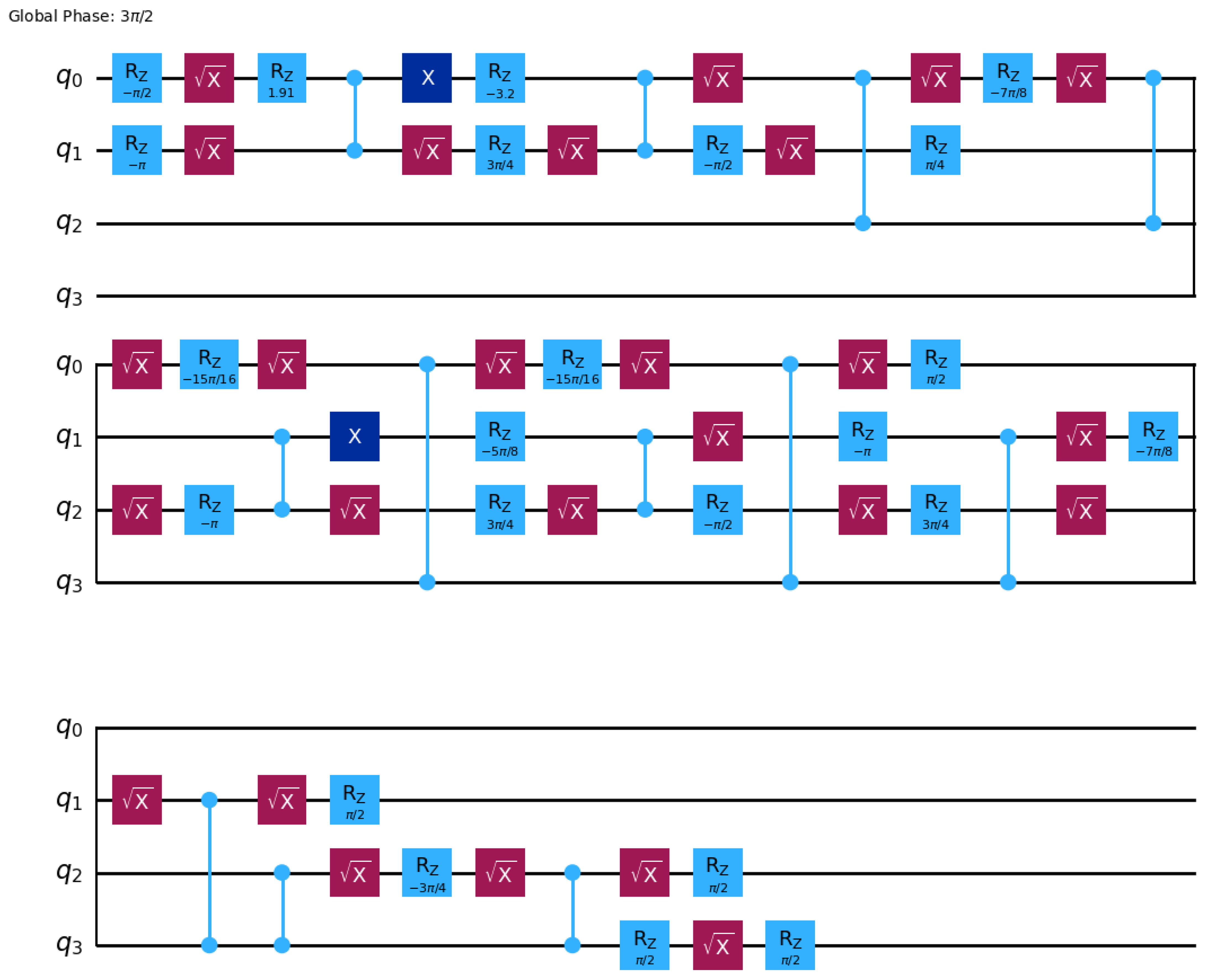
Following the procedure outlined in the previous sections, we compute the complexity of the three-qubit quantum Fourier transform. The complexity as a function of the penalty parameter can be seen in Figure 2. As the penalty parameter is increased the complexity increases also but reaches an asymptote close to C = 1.95 . As a point of comparison we have also computed the complexity of the three-qubit QFT by first transpiling to the gate set G = X , S x , R z ( θ ) , C z and using precomputed values of the complexity for these elementary gates to compute a baseline complexity. We call this the gate-sum complexity. The gate-sum complexity for the the three-qubit QFT has been numerically computed and is: C gatesum = 33.6 . The cost improvement gained by using a geometric compilation on the whole circuit instead of each individual gate and summing is 17.2 . The transpilation step for calculating the gate-sum complexity is done with the qiskit transpile function with optimization level = 3 and seed = 1 . The transpiled three-qubit QFT is shown in Figure A4.
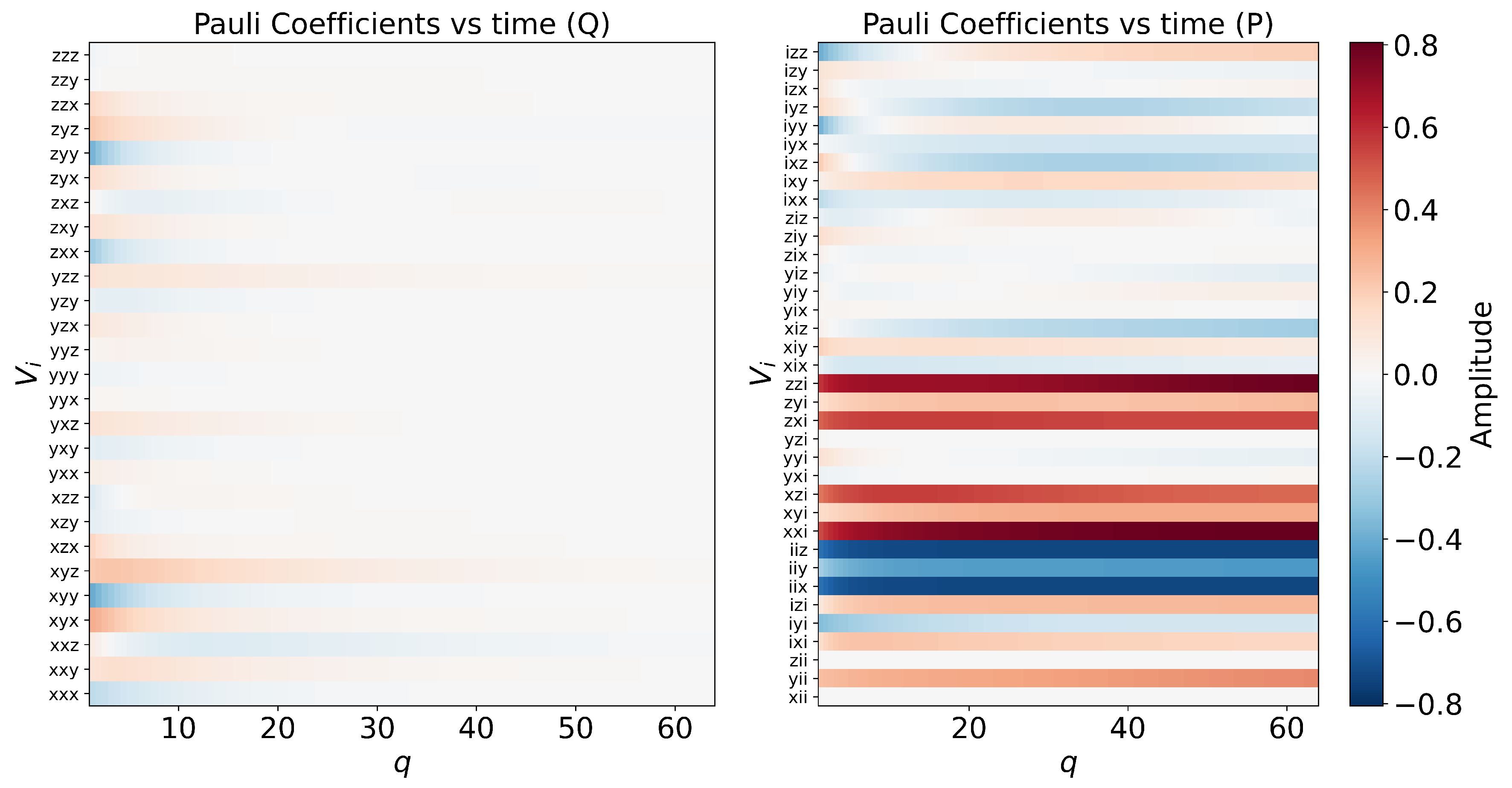
The initial Pauli coefficients for our Hamiltonian as a function of the penalty factor can be seen in Figure 3. In this figure, Pauli strings with weight higher than two are shown in red and labeled “Q”. We notice that as the penalty factor increases these penalized generators have shrinking amplitudes indicating that they are in fact being penalized by the algorithm. Moreover we note that the initial coefficients seem to be reaching steady-state values indicating our cutoff value for q is a reasonable one.
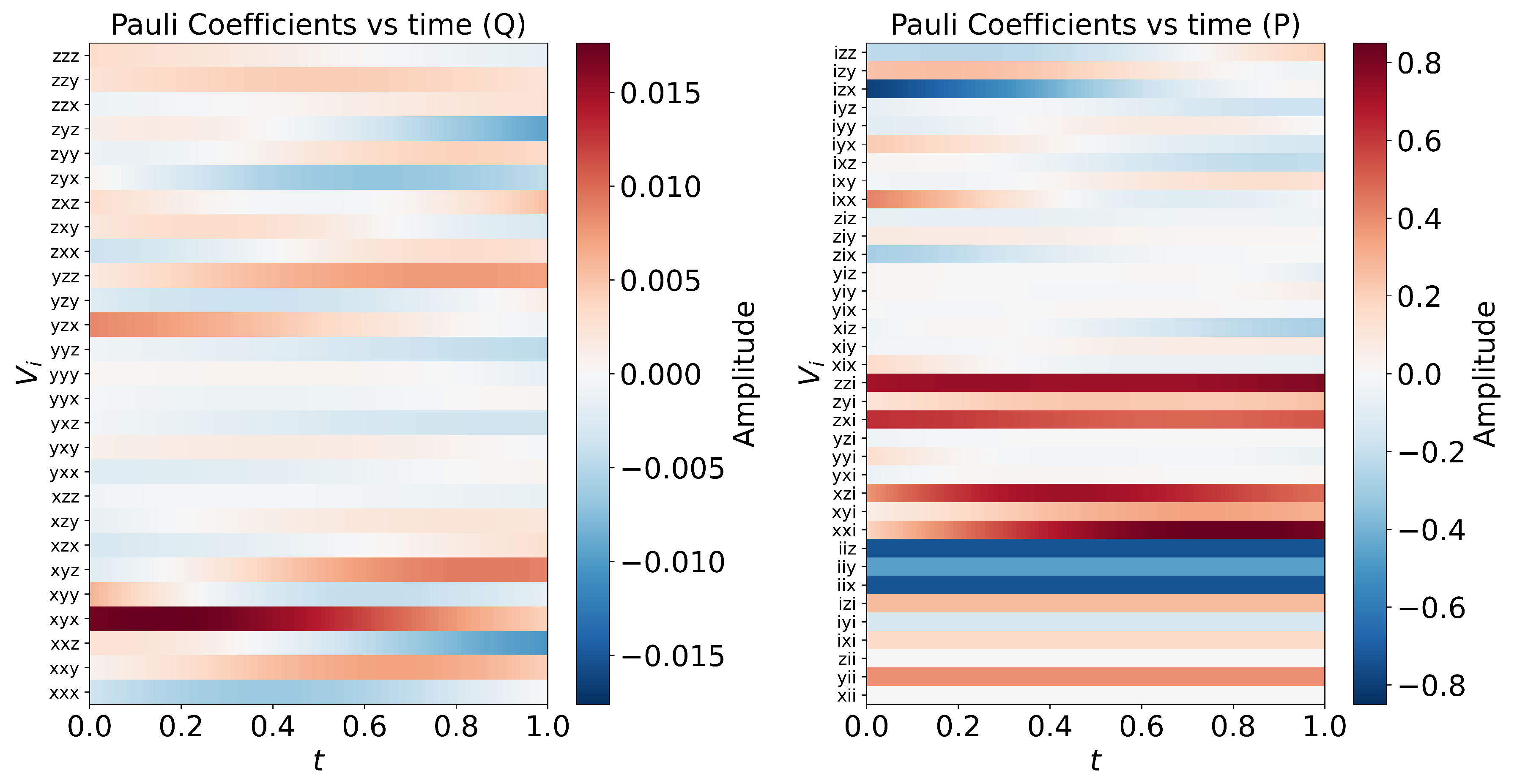
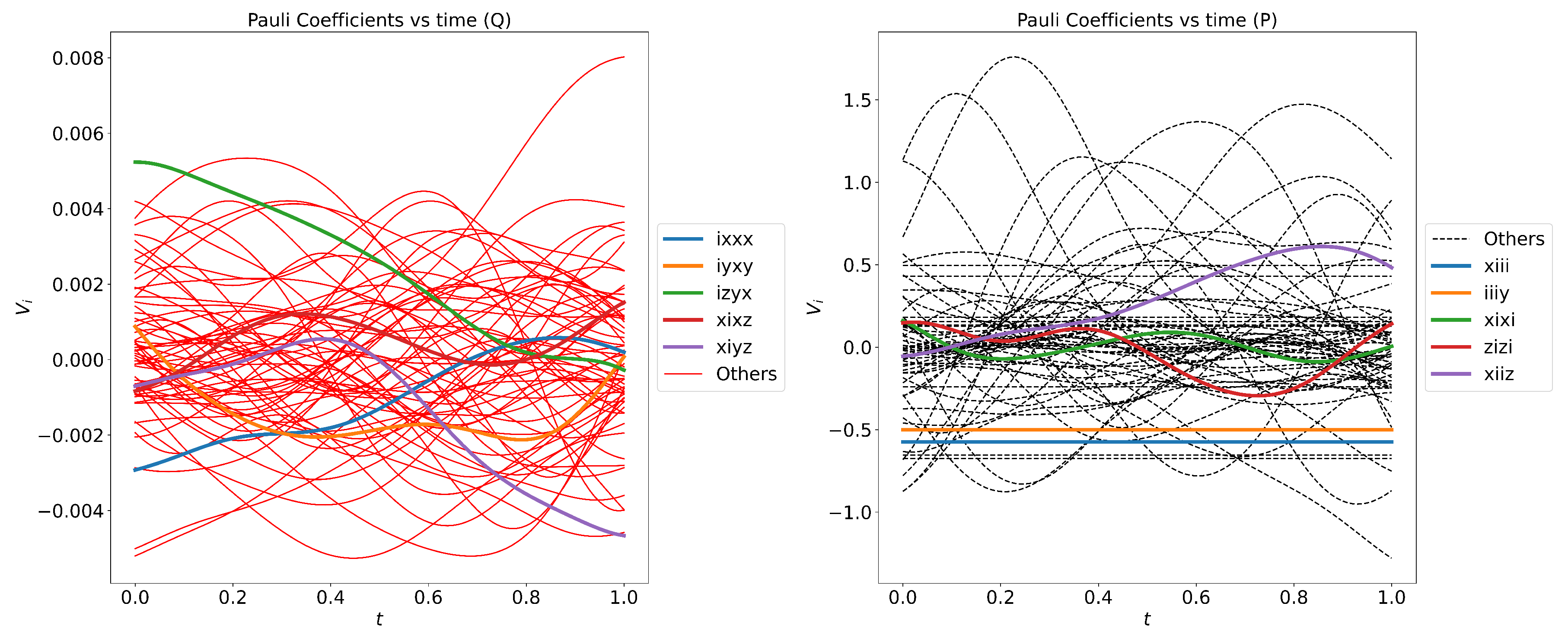
After having found the correct initial coefficients for our Hamiltonian, the geodesic equation can then be solved to obtain the time-dependent Hamiltonian coefficients. For this particular example the time-dependent coefficients can be found below in Figure 4. Geometrically these coefficients are interpreted as tangent vectors; from a quantum control perspective they are interpreted as control functions.
A concrete implementation of these coefficients on a quantum computer would require a quantum processor that is well modeled by the metric used here, or an adaptation of the code base to a metric that integrates more physical details of existing processors. A physical realization of such a procedure is beyond the scope of this report and we reserve it for later.
We have also repeated this analysis for the four-qubit quantum Fourier transform, which is shown in Figure A5. A transpilation of this circuit for the gate set G is shown in Figure A6. We find the complexity to be 3.29 and the control functions are shown in Figure 5. The gate-sum complexity of the transpiled circuit is 65.1. The gate-sum cost is a factor of 19.8 more than the geodesic compilation.
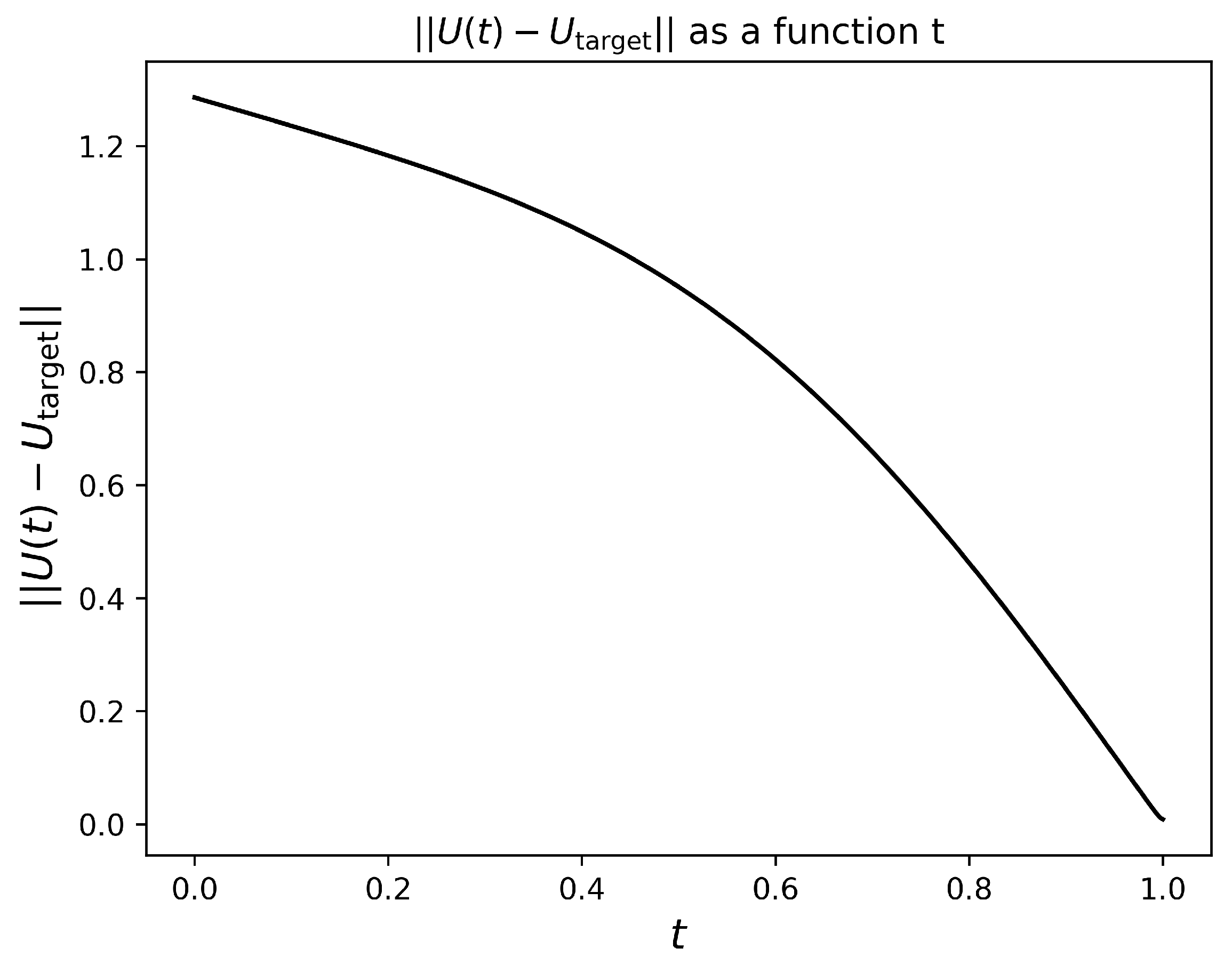
As a final step, we verify that the geodesic evolution of our unitary matrix indeed hits the target unitary. This can be checked by computing the rms deviation of our time-dependent unitary with the target unitary. That is, we compute | | U ( t ) U Target | | = 1 4 n U ( t ) U Target U ( t ) U Target for t 0 , 1 . Finally, we then plot this error function as a function of time. This plot can be seen below in Figure 6. We notice that the rms deviation approaches zero as time goes to 1, indicating that we are indeed hitting the target.
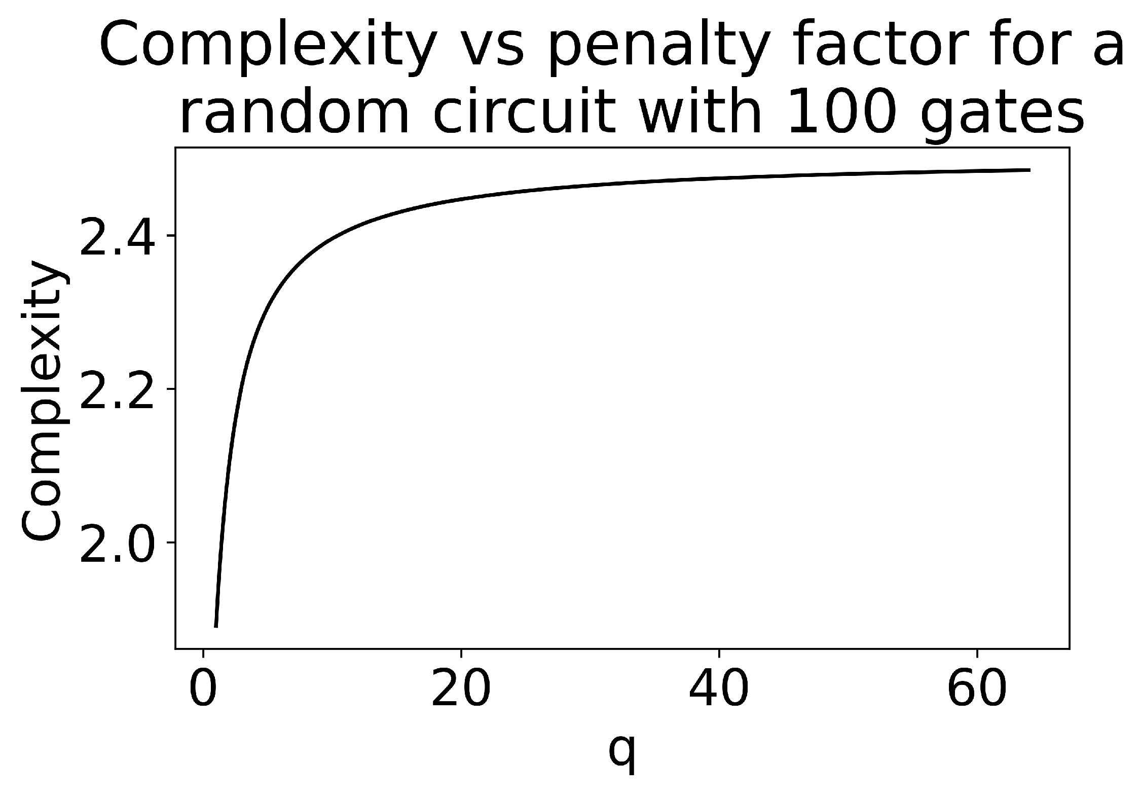
As a second example, we compute the complexity of a randomly generated quantum circuit with 3 qubits and a depth of 100, which can be seen in Figure A2. The circuit is composed of gates drawn from the gate set G. Gates and target qubits are drawn from this gate set with a uniform probability distribution specified by the numpy choice function. The seed for the choice function was set to be one. Our computation of the complexity of this quantum circuit as a function of the penalty factor can be seen below in Figure 7. We notice that the complexity is increasing with increasing penalty factor and reaches an asymptote close to C = 2.48 . Because this circuit is already expressed in terms of gates from G, no transpilation is needed and the gate-sum complexity is easy to compute. The gate-sum complexity of this circuit is found to be C RAND = 127.5 . So despite the perceived complexity of the circuit shown in Figure 7, it can actually be implemented with a 98 % cost reduction by compiling the whole circuit into geodesic control functions instead of compiling each gate independently. The saturation of the cost close to this low value is due to the dimension of the Hilbert space being only 2 3 for this three-qubit system.
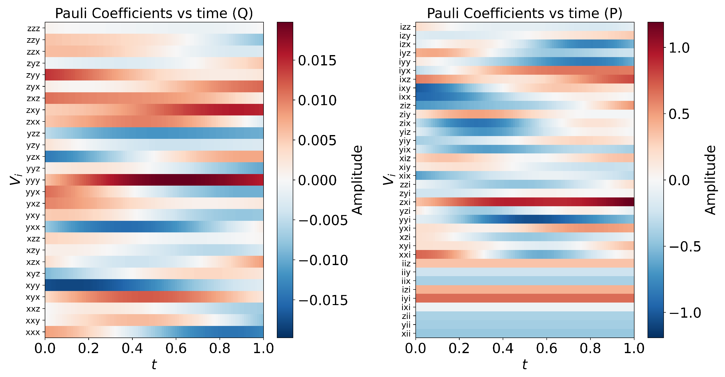
After having determined the initial values of the Hamiltonian for this randomly generated circuit, we then time-evolve the Hamiltonian to obtain its time evolution. The time evolution of the Hamiltonian coefficients can be seen in Figure 8. These coefficients are considerably more complicated-looking than the ones found in the case of the quantum Fourier transform, and have a larger amplitude, resulting in a complexity that is larger.
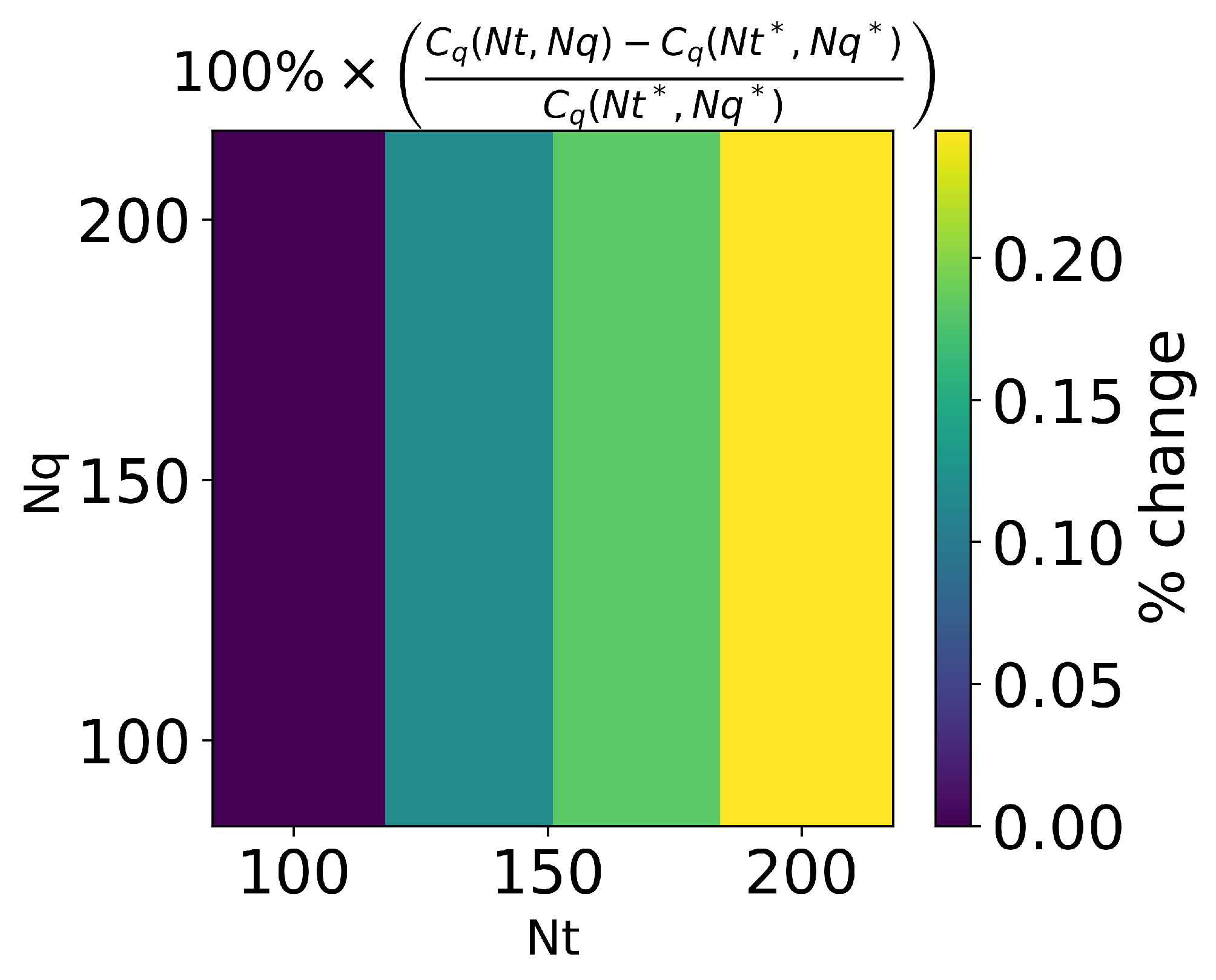
Convergence testing for this circuit was performed and it was found that the results did not change appreciably when the hyperparameters N q , N t , rtol and atol were varied. N q was varied from 100 to 200 and N t was varied from 101 to 201. Over this section of the parameter space, the obtained value of the complexity varied by less than a quarter of a percent (see Figure A8). Additionally, rtol and atol were decreased by an order of magnitude, from 10 3 to 10 4 and 10 6 to 10 7 respectively. It was found that the complexity did not change appreciably under this parameter shift.
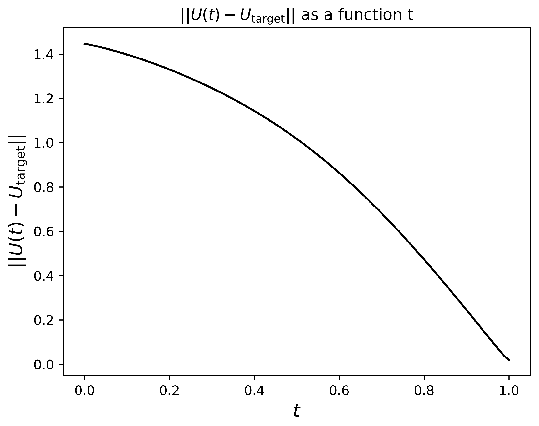
Finally, we compute the RMS deviation of our time-dependent unitary with the target unitary. The time-dependent RMS deviation can be seen below in Figure 9. Again, we are able to hit the target.

4.2. Fermion Chain Evolution

As a final example of our implementation of this algorithm, we calculate the quantum complexity of parts of a quantum circuit, which is used to calculate the evolution of a Hubbard model on a fermion chain. QGeo can only process a small number of qubits. However, we can use our method to reduce the depth of a large circuit if the circuit can be built by combining smaller circuits. As an example, let us consider a fermionic chain. In the case of non-interacting fermions, this chain is described by the Hamiltonian:
H Fermion = h i c i c i + 1 + c i + 1 c i .
Using the Jordan–Wigner transformation it is possible to express this Hamiltonian in terms of Pauli matrices acting at different sites, allowing for an implementation on a quantum computer. This transformation is given by:
c j = 1 2 σ j x i σ j y i < j σ i z , c j = 1 2 σ j x + i σ j y i < j σ i z .
we can represent the Hamiltonian in terms of Pauli operators
H Fermion = h 2 i σ i x σ i + 1 x + σ i y σ i + 1 y .
The time-evolution operator U ( T ) = e i H T can be approximated using Trotter–Suzuki decimation
U ( T ) t = 1 T / dt i e i h dt 2 σ i x σ i + 1 x e i h dt 2 σ i y σ i + 1 y ,
where the error in the approximation is O ( dt 2 ) . The evolution operator can be written in terms of commonly used quantum gates
U ( T ) t = 1 T / dt i R i , i + 1 x x ( h dt ) R i , i + 1 y y ( h dt ) .
The order of the products in Equation (40) can be rearranged without incurring error greater than O ( dt 2 ) . Circuits typically perform better if the gates are rearranged as
U ( T ) t = 1 T / dt ( i odd R i , i + 1 x x ( h dt ) R i , i + 1 y y ( h dt ) × i even R i , i + 1 x x ( h dt ) R i , i + 1 y y ( h dt ) ) .
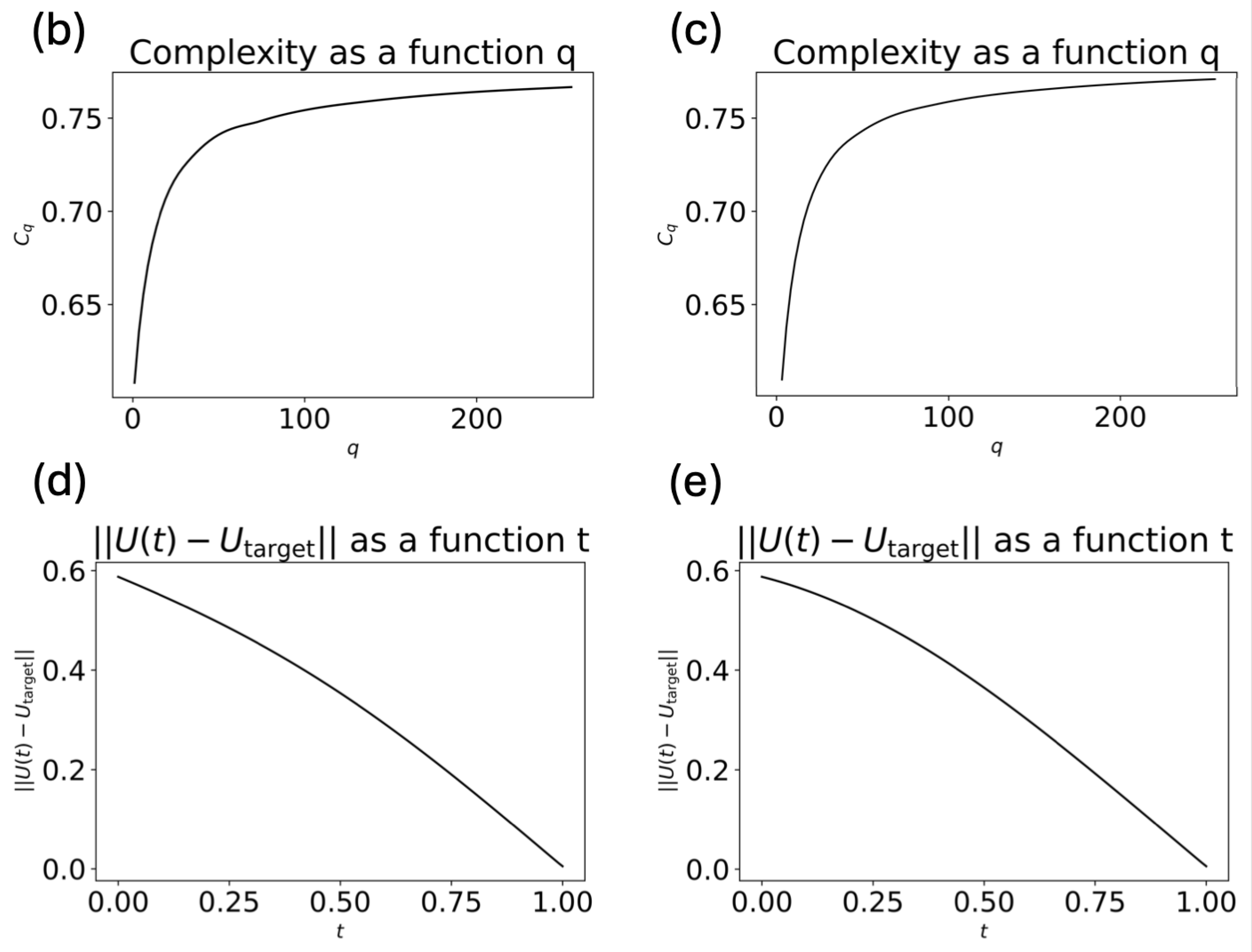
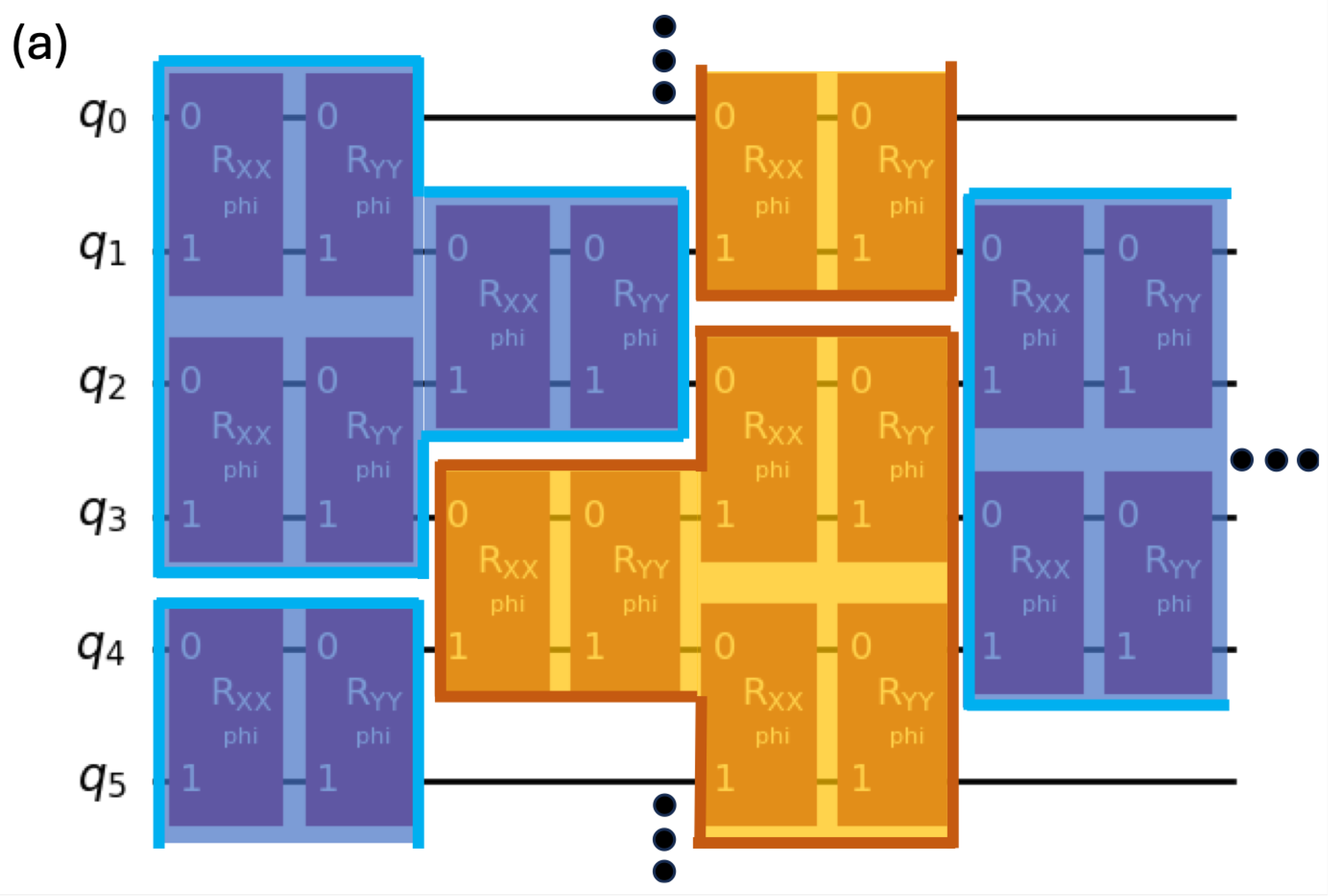
Figure 10a shows the corresponding quantum circuit. The circuit can be constructed out of two basic blocks shaded blue and yellow. By transpiling to the gate set, G, each R x x and R y y gate can be constructed using two CZ gates and several single-qubit gates. The transpilation of R x x is shown below in Figure A7. By using the analytic results from (32) it is possible to compute the gate-sum complexity analytically. We have C gate sum ( R x x ( θ ) ) = 6 π + 3 2 π + atan 2 sin ( θ ) , cos ( θ ) . Because each block in the Trotterized circuit consists of three R x x gates and R y y gates, the gate-sum complexity of the whole block is 6 × C gate sum ( R x x ( θ ) ) . For θ = 1 2 , the gate-sum complexity of the block therefore evaluates to C gate sum Block ( θ = 1 2 ) = 36 π + 3 3 π + 3 132.4 . However, from Figure 10b,c we see that when compiled with QGeo the entire block has a cost of only 0.77 . This is much lower than the calculated gate-sum complexity, highlighting inefficiencies for the naive implementation with respect to this metric. QGeo has the capability to detect such inefficiencies. The complexity of each block is reduced to only 0.6 % of the gate-sum complexity. This reduction carries over to the the full circuit. Thus, by building the circuit out of the reduced blocks, we are able to time-evolve fermionic chains for many more Trotter steps than would otherwise be possible in a time-constrained environment. Finally, in Figure 10d,e we see that the error from using the reduced block goes to zero.

5. Conclusions

In conclusion, we have developed a modern Python implementation of a method specified in [5,15] for determining geodesic control functions of quantum algorithms, called QGeo. Numerical methods must be used because analytic methods that can analyze geodesic complexities for circuits with more than two qubits are not available. Nevertheless, analytic methods are useful for obtaining complexities of one- and two-qubit gates, which can give context to the full numerical solutions. This implementation has been used to determine whether more efficient versions of quantum algorithms are available. Efficiency gains are quantified by comparing the geometric cost of the whole circuit with respect to the chosen metric, and the sum of the geometric costs of all gates in the circuit. In the case of the quantum Fourier transform, this Python package has shown cost reductions are available that can reduce complexities by about an order of magnitude compared with the textbook implementation. For quantum simulation of a fermionic chain, QGeo has been used to determine that more efficient implementations of Trotter blocks exist, which have a cost that is 99.4 % lower than the gate-sum complexity of the original implementation of the circuit. Therefore, while it is prohibitive to assess circuits with more than six qubits using QGeo, it is still possible to analyze and optimize circuits that have many more qubits, provided that they have a block type structure. In the case of the randomly generated circuit, our procedure was able find an implementation of the circuit that lowered the associated cost by two orders of magnitude.
These cost reductions can be realized at the abstract level where the metric used here is reasonable, however physical realizations are a current limitation. How one can implement an actual geodesic algorithm on an existing quantum processor is still not known. However, using the control functions obtained by QGeo and mapping them to existing quantum processors may be possible using more detailed knowledge of the actual processor architecture. This would however require modifications to the super-operator, G , to reflect characteristics of a given processor. These characteristics may include processor topology, error rates, practicality of pulses, robustness to noise, of pulses’ availability of single- and two-qubit Pauli strings, and mappings from RF pulses to Pauli strings. For example, processor topology could be implemented by penalizing Pauli strings corresponding to links outside the topology in the same way that three-qubit operations are penalized. This would likely lead to higher values of circuit complexities.
Extensions of QGeo that have better scaling properties to more qubits may be possible. This is because the space of tangent vectors with weight less than three only scales quadratically, whereas the full tangent space scales exponentially. This extension would require constrained optimization where tangent vectors are constrained to be on the space of two or fewer weight Pauli strings. However, a realization of better scaling is beyond the scope of this report and we reserve it for future work.   

Author Contributions

Conceptualization, S.T.C., J.P.T.S., J.N.P. and D.G.; Methodology, J.P.T.S.; Software, S.T.C., Z.L.B., J.A.D. and S.K.; Validation, J.P.T.S., S.K. and D.G.; Formal analysis, S.T.C. and J.J.L.; Investigation, S.T.C., J.P.T.S., Z.L.B., J.A.D. and D.G.; Writing—original draft, S.T.C., J.P.T.S., Z.L.B., J.A.D., J.N.P. and D.G.; Writing—review and editing, S.T.C., J.P.T.S., Z.L.B., J.A.D., J.N.P. and D.G.; Visualization, S.T.C.; Supervision, S.T.C.; Project administration, S.T.C. Funding acquisition, S.T.C. All authors have read and agreed to the published version of the manuscript.

Funding

This research was funded by Naval Information Warfare Center Pacific, grant number NISE Project 247.

Data Availability Statement

The original contributions presented in this study are included in the article. Further inquiries can be directed to the corresponding author. The Python package can be found at https://doi.org/10.5281/zenodo.19206495.

Acknowledgments

This work was funded by the NISE program at NIWC PAC. This work has also been supported by the Office of Naval Research (ONR) through the U.S. Naval Research Laboratory (NRL). We acknowledge QC resources from IBM through a collaboration with the Air Force Research Laboratory (AFRL).

Conflicts of Interest

The authors declare no conflicts of interest.

Appendix A

Generally solutions to the Schödinger equation can be found from:
U t = 1 + n = 1 i n 0 t d t 1 0 t 1 d t 2 0 t n 1 d t n H t 1 H t 2 H t n .
This can also be expressed as a time-ordered exponential that is a solution because:
i d U ^ d t = i d d t T e i 0 t d t H ^ ( t ) = i d d t T 1 + n = 1 n = 1 n ! ( i ) n 0 t d t 1 0 t d t n H ^ ( t 1 ) H ^ ( t n ) = i T n = 1 n = 1 n ! ( i ) n d d t 0 t d t 1 0 t d t n H ^ ( t 1 ) H ^ ( t n ) = i T n = 1 n = i = 1 i = n 1 n ! ( i ) n 0 t d t 1 0 t d t i 1 0 t d t i + 1 0 t d t n H ^ ( t 1 ) H ^ ( t i 1 ) H ^ ( t ) H ^ ( t i + 1 ) H ^ ( t n ) = H ^ ( t ) + H ^ ( t ) n = 2 n = 1 ( n 1 ) ! ( i ) n 1 0 t d t 1 0 t d t n 1 T H ^ ( t 1 ) H ^ ( t n 1 ) = H ^ ( t ) 1 + n = 1 n = 1 ( n ) ! ( i ) n 0 t d t 1 0 t d t n T H ^ ( t 1 ) H ^ ( t n ) = H ^ ( t ) U ^ .
Also, solutions to Schrödinger’s equation can be simplified through several different assumptions such as: 1. H is independent of time; 2. H is time-dependent but the Hs at different times commute; and the general case, case 3. The Hs at different times do not commute. Case 1 takes the form:
U t = exp i t t 0 H U 0 .
Case 2 takes the form:
U t = exp i t 0 t H t d t U 0 .
Case 3 takes the form:
U t = 1 + n = 1 i n 0 t d t 1 0 t 1 d t 2 0 t n 1 d t n H t 1 H t 2 H t n .
We usually will have each of the cases we have beginning at time t = 0 .
Finally, we list here the basis elements for Hamiltonians living in s u ( 2 ) , s u ( 4 ) and s u ( 8 ) . For notational convenience we suppress Kronecker products and sigmas. So for example in our notation we have x = σ x , and x I z = σ x I σ z . Given this notation we have the following basis sets:
x y z
I x I y I z x I x x , x y x z y I y x y y , y z z I z x z y z z
I I x I I y I I z I x I I x x I x y I x z I y I I y x , I y y I y z I z I I z x I z y I z z x I I x I x x I y , x I z x x I x x x x x y x x z x y I x y z x y y x y z , x z I x z x x z y x z z y I I y I x y I y y I z y x I , y x x y x y y x z y y I y y x y y y y y z y z I y z x , y z y y z z z I I z I x z I y z I z z x I z x x z x y , z x z z y I z y x z y y z y z z z I z z x z z y z z z
Figure A1. A flowchart showing the steps QGeo takes to calculate geodesics with respect to the metric G = P + q Q .
Quantumrep 08 00030 g0a1
Figure A2. A randomly generated circuit. Gates were drawn from the gate set G, with a uniform probability distribution. The numpy choice function was used to select gates from this set and also to select target qubits.
Quantumrep 08 00030 g0a2
Figure A3. The three-qubit quantum Fourier transform.
Quantumrep 08 00030 g0a3
Figure A4. The three-qubit quantum Fourier transform, transpiled into the gate set G, specified earlier. The qiskit transpile function was used to transpile the circuit in Figure A3 with optimization level 3 and seed equal to one.
Quantumrep 08 00030 g0a4
Figure A5. The four-qubit quantum Fourier transform.
Quantumrep 08 00030 g0a5
Figure A6. The four-qubit quantum Fourier transform, transpiled into the gate set G, specified earlier. The qiskit transpile function was used to transpile the circuit at Figure A5 with optimization level 3 and seed equal to one.
Quantumrep 08 00030 g0a6
Figure A7. A transpilation of the R XX θ into the gate set G.
Quantumrep 08 00030 g0a7
Figure A8. A sweep of of the hyperparameters, N t and N q , and the corresponding change in complexity. Complexity changes are measured relative to the complexity obtained at N t = 101 and N q = 100 .
Quantumrep 08 00030 g0a8

References

  1. Krantz, P.; Kjaergaard, M.; Yan, F.; Orlando, T.P.; Gustavsson, S.; Oliver, W.D. A Quantum Engineer’s Guide to Superconducting Qubits. Appl. Phys. Rev. 2019, 6, 021318. [Google Scholar] [CrossRef] [Scilit]
  2. IBM Quantum—IBM Torino. Available online: https://quantum.ibm.com/services/resources?tab=systems&system=ibm_torino (accessed on 26 February 2025).
  3. Brown, A.R.; Susskind, L. Complexity Geometry of a Single Qubit. Phys. Rev. D 2019, 100, 046020. [Google Scholar] [CrossRef] [Scilit]
  4. Wille, R.; Burgholzer, L. Machine Learning for Quantum Circuit Reliability. In 2023 International Symposium on Physical Design; IEEE: New York, NY, USA, 2023; pp. 198–204. [Google Scholar] [CrossRef] [Scilit]
  5. Nielsen, M.A.; Dowling, M.R.; Gu, M.; Doherty, A.C. Quantum Computation as Geometry. Science 2006, 311, 1133. [Google Scholar] [CrossRef] [Scilit] [PubMed]
  6. Goerz, M.H.; Basilewitsch, D.; Gago-Encinas, F.; Krauss, M.G.; Horn, K.P.; Reich, D.M.; Koch, C.P. Optimizing Quantum Control with Krotov’s Method. SciPost Phys. 2019, 7, 080. [Google Scholar] [CrossRef] [Scilit]
  7. Chowdhury, S.; Bojowald, M.; Mielczarek, J. Upper Bounds on Quantum Complexity of Time-Dependent Oscillators. arXiv 2024, arXiv:2407.01677. [Google Scholar] [CrossRef] [Scilit]
  8. Hackl, L.; Myers, R.C. Circuit Complexity of Free Scalar Fields. J. High Energy Phys. 2018, 2018, 139. [Google Scholar] [CrossRef] [Scilit]
  9. Camargo, H.A.; Hackl, L.; Heller, M.P.; Jahn, A.; Takayanagi, T.; Windt, B. Entanglement and Complexity of Purification in (1+1)-Dimensional Free Conformal Field Theories. Phys. Rev. Res. 2021, 3, 013248. [Google Scholar] [CrossRef] [Scilit]
  10. Chandra, A.R.; de Boer, J.; Flory, M.; Heller, M.P.; Hörtner, S.; Rolph, A. Spacetime as a quantum circuit. J. High Energy Phys. 2021, 2021, 207. [Google Scholar] [CrossRef] [Scilit]
  11. Flory, M.; Miekley, N. Complexity Change under Conformal Transformations. J. High Energy Phys. 2019, 2019, 003. [Google Scholar] [CrossRef] [Scilit]
  12. Flory, M.; Heller, M.P. Conformal field theory complexity from Euler-Arnold equations. J. High Energy Phys. 2020, 2020, 091. [Google Scholar] [CrossRef] [Scilit]
  13. Flory, M.; Heller, M.P. Conformal Field Theory Complexity and Holography. Phys. Rev. Res. 2020, 2, 043438. [Google Scholar] [CrossRef] [Scilit]
  14. Press, W.H.; Teukolsky, S.A.; Vetterling, W.T.; Flannery, B.P. Numerical Recipes: The Art of Scientific Computing, 3rd ed.; Chapter 18.1, The Shooting Method; Cambridge University Press: New York, NY, USA, 2007. [Google Scholar]
  15. Dowling, M.R.; Nielsen, M.A. The Geometry of Quantum Computation. Quantum Inf. Comput. 2008, 8, 861. [Google Scholar] [CrossRef] [Scilit]
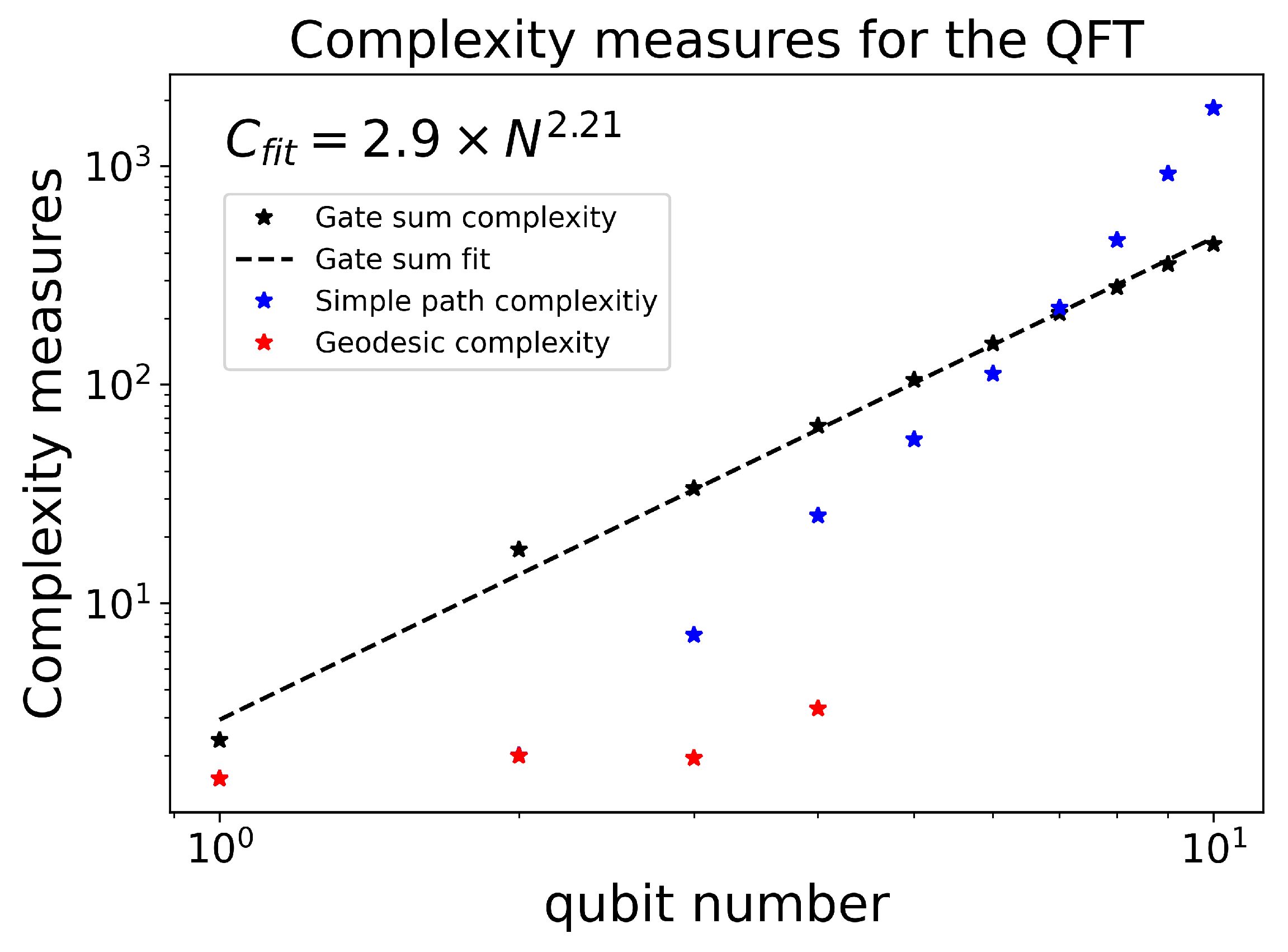
Figure 1. Comparison of simple complexity, numerical complexity ( q = 4 n case), and the gate-sum complexity for the quantum Fourier transform as number of qubits varies. The gate-sum complexity follows a trendline of C fit N 2.21 ± 0.06 . The computation for the three-qubit QFT ran in 17 s with a memory usage of 91 MB. The four-qubit QFT ran in 2100 s with a memory usage of 584 MB. Exponential scaling in time is expected because of the exponential size of the Hilbert space. All computations were performed on a Macbook Pro with an Apple M4 Max processor and 128 GB of RAM.
Quantumrep 08 00030 g001
Figure 2. The complexity of the three-qubit QFT as a function of the penalty factor. The complexity starts at a lower value corresponding to the simple-path complexity and then rises to an asymptote for higher penalty values.
Quantumrep 08 00030 g002
Figure 3. Initial coefficients of the Hamiltonian as a function of q, for the three-qubit QFT. These coefficients are such that under geodesic evolution the target unitary will be hit. Higher-weight qubit operators are being penalized and this is evidenced by their lowering amplitude as the penalty increases.
Quantumrep 08 00030 g003
Figure 4. Pauli coefficients of the Hamiltonian vs. time for q = 4 3 . The first pane shows Pauli coefficients that are penalized by the metric. These have a small amplitude, showing that they are being penalized. The second pane shows the unpenalized coefficients. These have a larger magnitude. In this pane a selection of Pauli coefficients are highlighted. We notice that two-qubit coefficients have non-trivial behavior and that single-qubit operations remain constant generally.
Quantumrep 08 00030 g004
Figure 5. Pauli coefficients of the Hamiltonian vs. time for q = 4 4 for the case of the four-qubit quantum Fourier transform. Again, higher weight Pauli coefficients are being penalized and so they have a lower amplitude. A selection of Pauli coefficients is highlighted in the second pane. We notice that two-qubit operations have non-trivial behavior and that single-qubit coefficients are constants.
Quantumrep 08 00030 g005
Figure 6. Verifying that the U ( t ) numerical solution evolves to U ( T ) = U ( 1 ) = U t a r g e t for the case of the three-qubit quantum Fourier transform when q = 4 3 .
Quantumrep 08 00030 g006
Figure 7. Complexity as a function of penalty factor for the randomly generated three-qubit, 100-gate circuit shown in Figure A2.
Quantumrep 08 00030 g007
Figure 8. Geodesic time evolution of the Hamiltonian coefficients at q = 4 3 for the randomly generated circuit shown in Figure A2. A consistency check here is that the penalized Pauli coefficients in the first pane have a small amplitude and the unpenalized coefficients in the second pane generally have a large amplitude. A selection of Pauli coefficients is highlighted. Two-qubit operations are generally non-trivial and single-qubit operations are generally constants.
Quantumrep 08 00030 g008
Figure 9. Verifying that the U ( t ) numerical solution evolves to U ( T ) = U ( 1 ) = U t a r g e t for the randomly generated three-qubit, 100-gate circuit shown in Figure A2.
Quantumrep 08 00030 g009
Figure 10. (a) Trotterized fermionic evolution circuit. The circuit is divided into two types of blocks. Block 1 is shaded blue and block 2 is shaded orange. (b) Complexity of the block 1 circuit as a function of q. (c) Complexity of the block 2 circuit as a function of q. (d) Error of the block 1 circuit as a function of time. (e) Error of the block 2 circuit as a function of time.
Quantumrep 08 00030 g010aQuantumrep 08 00030 g010b
Disclaimer/Publisher’s Note: The statements, opinions and data contained in all publications are solely those of the individual author(s) and contributor(s) and not of MDPI and/or the editor(s). MDPI and/or the editor(s) disclaim responsibility for any injury to people or property resulting from any ideas, methods, instructions or products referred to in the content.