Abstract
The nearest convex hull (NCH) classifier is a promising algorithm for the classification of biosignals, such as electroencephalography (EEG) signals, especially when adapted to the classification of symmetric positive definite matrices. In this paper, we implemented a version of this classifier that can execute either on a traditional computer or a quantum simulator, and we tested it against state-of-the-art classifiers for EEG classification. This article addresses the practical challenges of adapting a classical algorithm to one that can be executed on a quantum computer or a quantum simulator. One of these challenges is to find a formulation of the classification problem that is quadratic, is binary, and accepts only linear constraints—that is, an objective function that can be solved using a variational quantum algorithm. In this article, we present two approaches to solve this problem, both compatible with continuous variables. Finally, we evaluated, for the first time, the performance of the NCH classifier on real EEG data using both quantum and classical optimization methods. We selected a particularly challenging dataset, where classical optimization typically performs poorly, and demonstrated that the nearest convex hull classifier was able to generalize with a modest performance. One lesson from this case study is that, by separating the objective function from the solver, it becomes possible to allow an existing classical algorithm to run on a quantum computer, as long as an appropriate objective function—quadratic and binary—can be found.
1. Introduction
A promising study [1] established, for the first time, a method to produce accurate results with a 127-qubit computer. That work paved the way for near-term quantum applications and a new period, which is sometimes referred to as the “quantum utility era.” Quantum computing has provided similar or better results, compared to classical approaches, for certain optimization problems.
For example, ref. [2] demonstrated that quantum optimization can integrate with the Rosetta software for molecular design. In pharmacology, it is challenging to find a molecule that has the desired effect without any side effects and that is also easy to package and produce. The problem becomes exponentially complex as the size of the molecule increases. In contrast, quantum optimization performs consistently, regardless of the molecule’s size.
Quantum optimization yields distinct classification outcomes compared to its classical counterpart. In ref. [3], the authors studied the feasibility of quantum technology to detect fraudulent micropayment transactions. They identified the transactions for which classical and quantum classifiers disagreed and utilized those instances to train a meta-classifier. The meta-classifier was then used to select the preferred prediction in situations where the predictions from the quantum and classical classifiers differed. A key takeaway from the study is that quantum and classical approaches can detect different types of relationships. As a result, combining these approaches can enhance the classification performance.
Quantum machine learning has also provided excellent results in healthcare when classifying diabetes or heart disease, analyzing the impact of stress on mental health, and detecting Alzheimer’s or schizophrenia [4]. In ref. [4], it was shown that a quantum support vector machine (QSVM) using the correct set of hyperparameters—specifically, the feature map that determined the quantum kernel’s type—achieved a high classification score for detecting schizophrenia, based on an electroencephalogram (EEG) analysis.
Also in the domain of EEG analyses, ref. [5] demonstrated that quantum classification achieved excellent results when classifying resting states. Different resting states were induced by asking subjects to open or close their eyes. The algorithm then categorized the EEG signal epochs recorded during the two experimental conditions. The algorithm achieved a 99 % accuracy using only five qubits and limited preprocessing steps. Classification was performed on a time-sample-by-time-sample basis, and a principal component analysis (PCA) was used for a dimensionality reduction.
Similarly, ref. [6] provided a proof of concept for the quantum classification of EEG signals by computing symmetric positive definite (SPD) matrices and processing them using Riemannian geometry. The study focused on the P300, a potential elicited in the brain in response to a stimulation, which has a lower signal-to-noise ratio than data from resting states. The tangent space method based on Riemannian geometry was employed to generate feature vectors for each EEG trial epoch [7]. The feature vectors underwent an additional PCA to reduce their dimensions. The classifier was able to generalize, with results that were close to, but slightly lower than, those of the state-of-the-art linear discriminant analysis (LDA).
In this article, we focus on another classifier, called nearest convex hull (NCH) [8], which has been adapted to SPD matrices [9]. This is a supervised classifier where the label of a trial for classification is determined by calculating the Riemannian distance between the trial and the convex hull of the training trials. More precisely, the unidentified trial is assigned the label of the nearest hull in the Riemannian manifold. The optimization problem involves finding the point on the hull that is closest to the trial. We contributed additional classification strategies to the NCH. First, instead of using all training samples, we constructed the convex hull from only the N nearest samples. Second, we constructed K convex hulls per class, each based on N randomly selected samples.
This study assessed the performance of the NCH classifier for the classification of electroencephalography signals using a classical computer and a quantum simulator. In this study, we considered the dataset [10] to be a particularly challenging classification problem. It contained EEG recordings of participants alternating between two extremely similar resting states.
Another key challenge addressed in this study is the encoding of an optimization problem with continuous variables into an objective function that is quadratic, is binary, and accepts only linear constraints—in other words, an approach suitable for variational quantum algorithms. Our approach separates the objective function from the optimization techniques and demonstrates a promising avenue for translating an existing machine learning algorithm into one that can run on a quantum computer.
Note that the quantum computer or simulator was used exclusively to solve the optimization problem at the core of the classical machine learning algorithm. This represents a narrower scope within the broader field of quantum machine learning, as only the optimization routine is replaced by a quantum method, while both the model and data remain classical.
This approach of combining classical and quantum technologies is not entirely new, and several examples exist in the state of the art. For instance, ref. [11] proposed an enhanced variational quantum algorithm aimed at simulating the time evolution of large, uniform quantum systems with repeating structures. The core idea of their method is to determine optimal weights for a variational quantum circuit on small problem instances using classical resources. Once trained, these circuits are then scaled qubit by qubit to address larger instances of the problem.
In a similar vein, ref. [12] presented a hybrid classical–quantum approach in which a classical convolutional neural network (CNN) was trained to predict expectation values from random quantum circuits. This enabled the model to generalize to larger and deeper circuits, beyond the reach of current quantum hardware. A parallel can be drawn with Mozilla’s PRESC framework (accessed on 23 October 2025) https://mozilla.github.io/PRESC/) [13], which explores how classical machine learning models can replicate behaviors originally produced by black-boxed systems. While PRESC is typically applied in more traditional domains, ref. [12] embodied a similar philosophy for quantum computing. Another hybrid quantum–classical CNN approach is available in [14]. The authors proposed a framework designed to preserve image data privacy. It preserved the model’s accuracy while ensuring data privacy. These examples indicate that hybrid models represent an active field of research.
This paper is structured as follows. Section 2 introduces the NCH classifier, framed as a quadratic optimization problem, and background information on the quantum approximate optimization. Section 3 highlights our contribution. In particular, it describes the implementation of the objective function using a constraint-programming model and the process to solve this model using quantum optimization. Section 4 contains an experimental validation of the NCH on EEG data. Section 5 presents the results in comparison to the state-of-the-art method. In Section 6, we provide a comprehensive overview of our approach and recommendations, and Section 7 holds our conclusions.
2. Background
2.1. NCH Classifier
The NCH classifier [8] models each class by its convex hull. The NCH classifier is like k-NN at training time and stores only the training set in memory (Figure 1a). During classification, the matrix X to be classified is assigned to the class with the closest convex hull, denoted as :
The distance to the hull is the distance between X and the classification point . The classification point is the closest point on to X:
Note that the classification point depends on the test matrix X, as illustrated in Figure 1b, with a second test matrix.
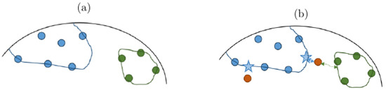
Figure 1.
Illustration of a binary classification using the NCH, where blue and green circles represent the two classes. (a) During the training phase of the NCH algorithm, the training set is stored in memory. (b) At classification time, a matrix to classify X (in orange) is assigned to the class with the closest hull. The classification point (blue star) depends on the matrix X, and is the point on the hull that is closest to X. Hulls are represented with curved lines to highlight that this NCH is applied on a Riemannian manifold.
Originally developed for Euclidean data, NCH was later extended to cover SPD matrices in [9]. Using a log-Euclidean distance, the classification problem can be explicitly written (see Equation (20) in [9]) as follows:
with and . In the above equation, denotes the matrix logarithm; X represents the matrix to be classified; is the index of the matrix belonging to class c; is the training matrix belonging to class c; and w is the weight that is optimized to find the classification point .
The objective function can be simplified as follows [9]:
as the term is constant. Note that the trace operator was omitted in Equation (21) of [9]. This objective function is a quadratic optimization problem that can be solved with constraint programming. However, it was not originally designed for EEG classification; to our knowledge, its application to an EEG analysis in this study is novel.
2.2. Quantum Approximate Optimization Algorithm
Quantum optimization algorithms are hybrid algorithms that rely partially on classical optimizers. In the field of quantum optimization, the main approaches are the variational quantum eigensolver (VQE) [15], the quantum approximate optimization algorithm (QAOA) [16], and quantum annealing (QA) [17]. The first two, VQE and QAOA, are very similar and belong to a family of variational quantum algorithms (VQAs). In contrast, QA falls under the category of simulated annealing algorithms. Strictly speaking, QA does not implement adiabatic quantum computing. More information is provided in Appendix A.
In this paper, we used QAOA as a quantum optimization algorithm. QAOA is a variational algorithm, originally designed to solve combinatory problems such as the MaxCut problem [16]. In other words, it integrates parameterized quantum circuits with classical optimization routines to solve quadratic, unconstrained, and binary optimization (QUBO) problems.
QAOA can be interpreted as a discretized approximation of adiabatic quantum computing (AQC). In particular, the unitary evolution operator derived from AQC (Equation (A3)) can be approximated using the Trotter–Suzuki expansion [18], as follows:
where and are non-commuting Hamiltonians, representing the initial (or mixer) and problem (or cost) Hamiltonians, respectively.
In QAOA, the ansatz is a parameterized quantum circuit constructed by alternating applications of the mixer and cost operators, repeated over n layers (see Figure 2). A classical optimizer is used to determine the optimal parameters and that minimize a given cost function.
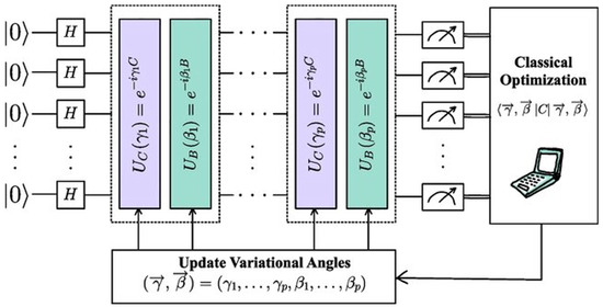
Figure 2.
Schematic representation of QAOA. The cost (C) and mixer (B) operators are illustrated in violet and cyan, respectively. Both operators are repeated p times. The terms and are the parameters. (Source: reproduced from [19].)
In the original implementation, the expectation value of the measured qubits was optimized. This expectation is always 0 and 1 on a universal computer. In contrast, the expectation can be continuous between 0 and 1 on a computer in which the registers are, or are equivalent to, harmonic oscillators, such as photonic or bosonic quantum computers. In our case, we were only interested in gate-based universal computers.
The cost operator was the Ising Hamiltonian of the QUBO problem. It was computed by mapping the terms of the objective function to a Pauli observable (i.e., a Hermitian matrix) [20], such as
We considered, as an example, the following objective function:
This Boolean function can be mapped to an Ising Hamiltonian using the following standard substitution:
where is the Pauli-Z operator acting on qubit i. The resulting Hamiltonian is
where is the identity operator acting on qubit i and ⊗ denotes the tensor product over the respective Hilbert spaces.
The mixer operator relies on the encoding scheme of the variables. As QAOA only works with QUBO problems, it is standard practice to convert integer or categorical variables into their binary form. By default, we used the X mixer, which is defined by the following Hamiltonian:
where N is the number of qubits and is the Pauli X operator acting on the ith qubit (indices starting at zero):
The X mixer performs the best when the variables are binary-encoded [21]. However, when the variables are encoded with one-hot encoding, we used the XY mixer, defined by
where is the Pauli Y operator acting on the ith qubit:
For domain-wall encoding, we used the domain-wall mixer, defined by
where is the Pauli Z operator acting on the ith qubit. Domain-wall encoding provides the best results for combinatory problems, such as workflow optimization [21].
In a quantum computer with registers functioning as harmonic oscillators, the qubit’s value oscillates between 0 and 1. Consequently, with a few adjustments to the mixer operator, one can optimize continuous variables using QAOA [22,23]. The QAOA then behaves as a quantum version of the gradient descent. On a gate-based quantum computer, this approach can be implemented by simulating registers with harmonic oscillators. An alternative method, proposed in [24], focuses on optimizing the quasi-probability distribution of the qubit rather than its expectation value. The motivation for this approach lies in the fact that the quasi-probability distribution is always continuous, whereas the expectation value on gate-based quantum computers remains binary. In the remainder of this article, we focus on this method and benchmark it against a naive implementation of QAOA for continuous variables, where continuous variables are simply encoded into binary variables and optimized using the original QAOA. These approaches are described in more detail in Section 3.3 and Section 3.4.
In conclusion, the performance of QAOA relies on the selection of both the mixer operator and classical optimizer. In [25], various classical optimizers were benchmarked for QAOA, and gradient-based algorithms such as Adam and Powell, as well as COBYLA and the SPSA, achieved solutions with the lowest energy values. SLSQP was also reported as a competitive option, being the fastest among all the tested optimizers. This speed advantage may allow SLSQP to perform more iterations within the same time budget, potentially leading to lower energy values. However, the results in [25] were obtained using a quantum simulator with only the noise model of a five-qubit quantum device (IBMQ Rome). For experiments on real quantum hardware or extremely noisy quantum simulators, a simultaneous perturbation stochastic approximation (SPSA) [26,27] may be a more suitable choice, as it is specifically designed to operate effectively in noisy environments.
3. NCH Implementation for Quantum Computing
For our quantum implementation, we employed constrained optimization methods, which enabled the use of both the naïve implementation of QAOA-CV and the QAOA-CV variant with quasi-probability distribution optimization. We used the SLSQP optimizer, except for QAOA-CV, where the SPSA algorithm was applied. In this section, we explore the NCH model and its adaptation, selecting the most suitable quantum encoding strategy. Next, we address every aspect of this implementation in detail.
3.1. Constraint-Programming Model
Constraint programming is a declarative programming paradigm for representing complex problems by defining variables and their relationships. This results in an objective function along with a set of constraints. An optimizer then searches for solutions that minimize or maximize the objective function while satisfying all constraints.
The core idea is to promote optimization expressiveness by decoupling the problem definition from the solving strategy. This separation enables the use of various, potentially novel or specialized, optimization techniques to solve the same problem formulation.
DOcplex [28] is IBM’s modeling framework, used here to define a quadratic optimization problem through constraint programming. DOcplex aids in converting a mathematical problem into an objective function that can be further optimized. The mathematical problem considered in this case was the NCH quadratic problem, which is utilized in Equation (4) with the log-Euclidean distance, where w is the variable to optimize.
This problem admits a linear constraint whereby the sum of the weights must be equal to 1. However, because QUBO problems do not support constraints, a penalty term was added to the objective function. This term heavily penalizes any violation of the constraint, so the solver is guided toward feasible solutions. We used the LinearEqualityToPenalty converter [29], which automatically converts a linear equality constraint into such a penalty term. The objective function in Equation (4) can then be rewritten as follows:
where is the penalty coefficient. The idea is that any solution for which the weights do not sum to 1 incurs a large penalty, making it unlikely to be selected when minimizing the objective function. In our case, was computed as follows:
where and denote the upper and lower bounds of the linear objective terms, and and refer to those of the quadratic terms.
This objective function is straightforward to implement with DOcplex using the sum method and DOcplex variables to represent the weights w (Listing 1). The variable type can be either continuous, integer, or binary, depending on the optimization method used (naïve QAOA, QAOA-CV, or classical).
| Listing 1. Definition of the objective function with DOcplex. |
 |
In pyRiemann-qiskit, this type is managed by an instance of pyQiskitOptimizer, which employs the correct variable type and, if necessary, converts the problem into QUBO. The convex distance of the NCH was implemented through constraint programming using DOcplex, and the implementation is available in pyRiemann-qiskit [30].
3.2. Quantum Implementations of NCH
In the NCH algorithm, each point in the training set is associated with a weight that must be optimized. Consequently, the complexity of the problem increases with the size of the training set.
In the context of quantum computing, each weight is ultimately encoded into one or more qubits, which imposes strict constraints on the size of the dataset. Quantum simulators have a maximum capacity of 36 qubits, meaning that, in the best-case scenario—where each weight is represented by a single qubit—these simulators can handle convex hulls containing up to 36 matrices. However, approaching this upper limit is not advisable, as the simulation time grows exponentially with the number of qubits, making such experiments computationally impractical.
For this reason, the NCH module in pyRiemann-qiskit implements the following two strategies to avoid estimating the hull on all matrices of each class:
- Min hull: The min hull finds the matrices closest to the test matrix and uses them to estimate the hull of the class.
- Random hull: The random hull randomly samples subsets of training matrices to construct multiple convex hulls per class, each based on fewer points. For a given test sample, the distances to all hulls within each class are computed and summed, resulting in an aggregate distance per class. The class with the minimum aggregate distance is then assigned as the label for the sample.
The number of hulls and samples per hull are controlled by the parameters of the NCH implementation.
3.3. Naïve Implementation of QAOA-CV
QAOA-CV stands for “quantum approximate optimization algorithm with continuous variables.” This version is an extension of the original QAOA that allows for handling not just binary variables, but also continuous ones. A straightforward implementation of QAOA-CV involves transforming continuous variables into binary ones.
The algorithm comprises two steps:
Step 1: Discretization of Continuous Variables
Each continuous variable in the objective function is transformed into a bounded integer variable . The lower bound of is fixed at 0, while the upper bound is arbitrarily defined and determines the precision of the representation.
Formally,
The mapping between and can be expressed as follows:
As increases, the discretization becomes finer, thereby enhancing the precision of the continuous variable’s representation.
Example 1.
Consider a continuous variable . If its integer representation is defined by , then
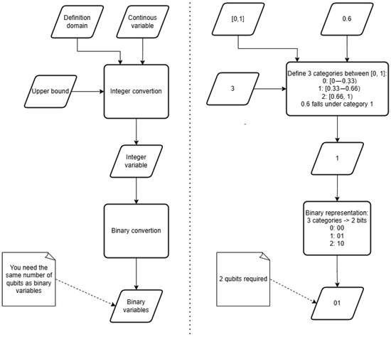
As shown in Figure 3, a value of 0.6 falls into category 1. Increasing the upper bound (e.g., from 3 to 10) allows for a more granular mapping between x and z.
Figure 3.
Flow diagram depicting the algorithm for encoding continuous variables into binary ones. First, continuous variables are mapped to integers by dividing their domain into a fixed number of intervals. This mapping depends on the definition domain of the continuous variable and the chosen number of intervals (upper bound). Second, the resulting integer values are encoded into binary ones using, for example, their binary representation. The diagram on the right illustrates how to encode the value 0.6, defined over the interval [0, 1], into a binary number using the proposed method.
Step 2: Encoding for Quantum Representation
Each integer variable is subsequently encoded into binary variables to enable processing by the QAOA. This step establishes the connection between the discretized classical variables and their quantum representation by mapping each integer value to a unique binary string. As shown in Figure 3, each category obtained in the previous step is assigned a binary representation using the binary encoding scheme, allowing QAOA to operate directly on the encoded variables.
Remark 1.
In general, the encoding can be implemented using one of several techniques, including the following:
- Binary encoding;
- One-hot encoding;
- Domain-wall encoding [21].
We selected binary encoding and now provide the rationale for this choice. Each binary variable generated through this algorithm requires a separate qubit. Consequently, the total number of qubits required by QAOA scales with both the number of discretized variables and the chosen encoding scheme. Quantum simulations typically strive to minimize the number of qubits used, which makes it crucial to select an efficient encoding strategy and set a proper upper bound. For instance, integer variables ranging from 0 to 3 (upper bound = 3) can be represented using one-hot encoding with three bits (e.g., 001, 010, 100), or more efficiently with binary encoding using only two bits (00, 01, 10, 11). In contrast, variables ranging from 0 to 15 (upper bound = 15) require 4 bits with binary encoding, but as many as 15 bits with one-hot encoding. This illustrates the importance of selecting a compact representation to balance precision and quantum resource constraints. To balance the precision and resource constraints, we adopted binary encoding and set the upper bound of the integer variable to 7 by default, allowing for eight distinct categories. This decision represents a practical compromise that ensures adequate precision while keeping the computational costs low.
Example 2
(with NCH). If there are two training points, the weight vector will consist of two variables. Each variable can take integer values between 0 and 7, requiring three qubits to encode each value ( possible values). Consequently, the total number of qubits needed is .
A notable advantage of binary encoding is its efficiency in qubit usage when the upper bound is high. For instance, representing eight categories using one-hot encoding would require eight qubits per weight. In contrast, binary encoding achieves the same representation with far fewer qubits (only three, as we saw).
In the remainder of this article, the X mixer was utilized to encode the continuous variables, and we employed the SLSQP algorithm to optimize the weights of the QAOA ansatz.
3.4. QAOA-CV with Quasi-Probability Distribution Optimization
QAOA focuses on optimizing the expectation values, which are typically and , for a universal quantum computer. The current implementation of QAOA-CV was proposed in [24] and focuses on the optimization of the quasi-probability distribution, which is continuous.
In this case, we simply replaced the continuous variables with binary ones. This is a formal modification that allows us to compute the cost operator as if the variables are binary. The cost operator is therefore the same as if the problem were just a QUBO problem. We then optimized the parameters of the circuit, based not on the expectation values, but rather on the quasi-probability distribution. For example,
- There are two variables, a and b.
- Each variable is represented by one qubit.
- The optimizer adjusts the parameters, and we measure the qubits, which yields the following distribution:
The quasi-probability of the first (resp. second) qubit being in state is 0.5 (resp. 0.6). Therefore, we retain 0.5 and 0.6, respectively, as the new values for variables a and b. This approach differs from classical QAOA, which optimizes the expectation value , where is the most probable state (e.g., ) and is the cost Hamiltonian. In our case, the expectation value becomes
where f is the cost function.
In [24], the SPSA was shown to perform well as a classical optimizer for determining the weights of the QAOA ansatz, whereas SLSQP failed to converge. This is noteworthy, as SLSQP was the recommended optimizer for the naïve implementation of QAOA-CV.
While [24] does not provide a theoretical framework to explain this discrepancy, it is important to emphasize that the cost function described above differs from that of QAOA. As a result, the implementation presented in [24] shares the ansatz and algorithm name with QAOA, but not the exact mathematical formulation.
4. Experiments
4.1. Data
The classification of resting states falls under the domain of passive brain–computer interfaces (BCIs), which involve responsive interfaces that monitor and adjust to the user’s cognitive state without requiring their active participation [31].
We utilized the Cattan2019_PHMD dataset [10] for passive music listening, accessible through MOABB [32,33]. The data comprise EEG recordings from twelve healthy subjects (three females) who had a mean age of 26.25 years (standard deviation: 2.63 years). The EEG signals were captured using the EC20 cap equipped with 16 wet electrodes (EasyCap, Herrsching am Ammersee, Germany), placed according to the 10–10 standard. The reference was placed on the right earlobe, and the ground was placed at the AFz scalp location. The amplifier was linked via a USB connection to a personal computer on which the data were recorded, using the software OpenViBE [34,35]. The data were acquired without digital filtering, using a sampling frequency of 512 samples per second.
For all participants, the experimental task involved listening to music, both with and without a passive head-mounted display. A passive head-mounted display has no electronics other than a smartphone. The experiment consisted of ten blocks: in five blocks, the smartphone was switched off, and in the other five, it was switched on. Each block consisted of 1 min of EEG data recording with the subject’s eyes open. A total of 10 min was thus recorded for each subject. The sequence of the ten blocks was randomized prior to the experiment.
The resulting dataset poses a classification challenge, as [36] found no significant differences in the power signal of the two experimental conditions for the same subject. As a result, state-of-the-art EEG classification methods (e.g., Riemannian methods like the MDM [37]) fail to distinguish epochs of signals recorded when the participant is wearing or not wearing a head-mounted display.
To provide a point of comparison for the interpretation of the results thereafter, Riemannian classification pipelines typically report area under the ROC curve (AUROC) values ranging from 0.7 to 0.95 [38], depending on the paradigm and the dataset. For the classification of resting states, the same methods achieve an AUROC close to 1 with [39]. In contrast, the AUROCs found in the Results section (Section 5), using the same methods, are low, with values reported below 0.6.
4.2. Preprocessing
The data were resampled to 128 Hz, and we applied a bandpass filter between 1 and 35 Hz. For each trial, composed of 16 channels, we extracted an epoch lasting 40 s and starting 10 s after the onset of the trial. No artifact removal was applied. The EEG epochs were transformed into SPD matrices, as detailed below.
- For each signal epoch S (n_channels x n_samples), a covariance matrix X (n_channels × n_channels) was estimated that was, by definition, symmetric:after centering the signal S. See [40] for other covariance matrix estimators.
- With sufficient time samples, the covariance matrices become SPD, or otherwise, they must be regularized. Regularization was achieved by computing the shrunk Ledoit–Wolf covariance matrix of the epoch [40].
- The space of SPD matrices is a manifold with a more intricate geometry than that of the Euclidean space.
- The manifold becomes a Riemannian manifold when endowed with an affine invariant metric, where each covariance matrix becomes a point on this manifold.
In summary, each trial was transformed into a covariance matrix of size 16 × 16. We can now apply a classifier to this manifold. In this study, we considered the NCH and two classifiers based on Riemannian geometry executed on a non-quantum computer. First, the minimum distance to mean (MDM) [37] is a popular classifier that assigns an SPD matrix to the class according to the nearest mean on the manifold. Second, tangent space + LDA (TS + LDA) [41] is a state-of-the-art classifier that projects the SPD matrices onto the tangent space of the manifold and then applies a linear discriminant analysis (LDA) for classification. The LDA projects data into a lower-dimensional space while maximizing the separability between classes, assuming that they follow a normal distribution with a common covariance matrix, which allows for a linear decision boundary. The choice of these algorithms comes from the EEG benchmark [38]. Together, these two classifiers establish a robust baseline against which the performance of our new NCH implementation can be compared.
4.3. Pipelines
We then tested the following eight different classification methods:
- NCH + MH: NCH classifier with min hull subsampling. We used SLSQP as a classical optimizer.
- NCH + RH: NCH classifier with random hull subsampling. We used SLSQP as a classical optimizer.
- NCH + MH_NAIVEQAOA: NCH classifier with min hull subsampling. We used the naïve implementation of QAOA-CV with SLSQP as an optimizer, and the mixer operator was the X mixer.
- NCH + MH_QAOACV: NCH classifier with min hull subsampling. We used QAOA-CV (with quasi-probability distribution optimization) using SPSA as an optimizer, and the mixer operator was the X mixer.
- NCH + RH_NAIVEQAOA: NCH classifier with random hull subsampling. We used the naïve implementation of QAOA-CV with SLSQP as an optimizer, and the mixer operator was the X mixer.
- NCH + RH_QAOACV: NCH classifier with random hull subsampling. We used QAOA-CV (with quasi-probability distribution optimization) using SPSA as an optimizer, and the mixer operator was the X mixer.
- TS + LDA: 16 × 16 covariance matrices were projected from the SPD manifold to the tangent space, resulting in vectors of dimension 136 = 16 × (16 + 1)/2). These vectors were then passed as input to an LDA classifier [41].
- MDM: Direct classification of 16 × 16 covariance matrices in the SPD manifold with the Riemannian mean and distance [37].
For optimizers of NCH classifiers, we set the number of maximum iterations to 100. For MIN_HULL-based NCH classifiers, we set the number of samples to six. For RANDOM_HULL-based NCH classifiers, the number of hulls and samples per hull were set to three and six, respectively. The number of repetitions for the QAOA ansatz was set to two.
4.4. Evaluation
We used a cross-subject evaluation with three splits, using the standardized implementation available in MOABB. This implementation uses group k-fold validation (non-stratified), with three folds. The AUROC was used as the classification metric.
The global seed for the Qiskit algorithm module, the random seed for the quantum transpiler (which compiles the Python code into the quantum circuit assembly) and simulator, and the seed for the NumPy and random Python modules were all set to 475,751. This seed corresponds to the one generated the first time we ran our code.
For research reproducibility, the code we used is available at https://github.com/pyRiemann/pyRiemann-qiskit/blob/main/examples/resting_states/noplot_nch_study.py (accessed on 23 October 2025). It uses pyRiemann-qiskit 0.4 [30], pyRiemann 0.8 [42], Qiskit 1.2 [43], Qiskit Optimization 6.3.1 [29], and Qiskit Machine Learning 0.7.2 [44]. We used Qiskit-Aer 0.15 [45] to simulate a quantum computer, employing an ideal quantum circuit state-vector simulator.
5. Results
Figure 4 displays the results obtained from classical optimization. The scores and times for all pipelines, shown as the averages across all sessions, are listed in Table 1.
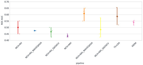
Figure 4.
Scatter plots: AUROC per pipeline. Each point represents a session in the dataset.

Table 1.
AUROC values and time (in seconds) for all pipelines, averaged across all sessions. The time is the average time by fold. All NCH pipelines were multi-threaded, with a default of 12 threads, whereas TS + LDA and MDM were single-threaded. Note that the actual time depends on the capabilities of the machine, such as the number of cores, their speed, and the available RAM.
As the dataset presents a significant classification challenge, lower performance results were anticipated.
We calculated the chance level for the Cattan2019_PHMD dataset. At an alpha value of 0.05, significance was attained when AUROC = 0.5833 or at 70 correct classifications. The significance threshold is reported here in accordance with the standards commonly used in the EEG field [46,47]. Only two pipelines, namely TS + LDA (AUROC = 0.59) and NCH + MH_NAIVEQAOA (AUROC = 0.61), were significantly better than the chance level (AUROC = 0.5833).
The main takeaways are, firstly, that NCH is able to extract valuable information from the data in cases where classes are difficult to distinguish and the MDM struggles to generalize.
Secondly, the quantum-optimized pipeline NCH + MH_NAIVEQAOA ranked first and performed slightly better than the state-of-the-art TS + LDA. While the results are encouraging, it should not be interpreted as exceeding the current state of the art.
Third, the non-quantum version of the NCH performed worse than the quantum-enhanced versions.
Considering the classification difficulty of the selected dataset, and because the observed values were close to chance and relatively similar across pipelines, we did not perform statistical significance testing—such as permutation tests—to assess the differences between them, as meaningful results were not anticipated.
The reader is referred to Appendix B to gain a deeper understanding of the behavior of the NCH algorithm when the number of hulls and samples were varied.
6. Discussion and Limitations
The approaches presented in this article warrant further investigation due to several limitations. First, the naïve QAOA approach relies on solving QUBO problems, which necessitates encoding continuous variables into binary representations. In our study, this was achieved by fixing an arbitrary precision and upper bound. While increasing the upper bound allows for finer precision, it also substantially increases the number of quantum bits required to encode the weights. Alternative encoding methods, such as fixed-point, one-hot, or domain-wall encoding [21], may offer advantages that were not explored here, given the limited scope of this article.
Secondly, the number of weights required for QAOA-CV is directly proportional to the number of samples used for training. As a result, the memory demands and computational costs increase as a function of the dataset’s size. This scaling makes the method in its current form practical only for small datasets, especially during simulation.
Third, this study employed only a quantum simulation instead of a real quantum computer. Simulations provide an understanding of the algorithm’s behavior, but they do not incorporate the practical constraints and challenges that arise when using real quantum hardware. In practice, quantum computers are subject to various sources of noise—such as topological and environmental noise—that cause the decoherence of the quantum state and introduce measurement errors. Additionally, the naïve QAOA algorithm does not scale efficiently, as the number of qubits increases exponentially with the upper bound applied during binary encoding. Consequently, QAOA is currently practical only for small datasets, whether executed on a simulator or on real quantum hardware, typically limited to 127 qubits at the time of writing. Another constraint that arises when using real quantum computers is the waiting time before a computation is executed on the quantum device. This waiting time depends on the number of concurrent users and user privileges. This limitation alone currently makes real quantum computers impractical for online classification tasks.
Fourth, these results were contingent on the random seed we chose at the beginning of the experiment, as well as the shuffle performed during the group three-fold validation. Hence, the results are only valid for a specific setup. Additionally, we utilized cross-subject validation, which involves the challenging task of transfer learning between sessions and subjects, in a dataset where the two experimental conditions are not easily distinguishable.
7. Conclusions
This paper advances the field through the following three contributions.
First, we contributed our own implementation of the nearest convex hull (NCH) algorithm, enhanced with two additional strategies for the construction of convex hulls and subsequent classification, that can better handle different datasets.
Second, we outlined the fundamental steps required to adapt an existing classical algorithm for quantum processing. Using the NCH algorithm as a case study for bio-signal data classification, we achieved this adaptation by reformulating the algorithm as an optimization problem via constraint programming. This reformulation made the algorithm compatible with the QAOA optimizer, which operates on QUBO problems. In summary, the optimization problems we defined are quadratic, accommodate only linear constraints, and involve converting continuous variables into binary ones. In addition, we also introduced an original approach to QAOA-CV, focusing on the optimization of the quasi-probability distribution of binary variables. This adaptation is versatile and can be applied to a wide range of optimization problems and domains, beyond the scope of the NCH algorithm.
Third, we also evaluated for the first time the performance of the NCH classifier on EEG data. Our results show that it is a promising algorithm for cross-subject classification with resting-state data, particularly when combined with quantum optimization. On this dataset, the NCH + MH_NAIVEQAOA variant approached the performance of the state-of-the-art TS + LDA method and performed rather better than the MDM. Note that TS + LDA operates in the tangent space of the Riemannian manifold, while both MDM and NCH perform classification directly on the manifold. There remains room for improvement, however, as both NCH + MH_NAIVEQAOA and TS + LDA achieved classification accuracies only slightly above the chance level for this dataset.
Consequently, it is difficult to draw definitive conclusions regarding the conditions under which quantum optimization may outperform its classical counterparts. We note, however, that the dataset is relatively small and that the classification task is particularly challenging. In other words, potential quantum advantages are more likely to emerge in scenarios where classical approaches struggle to provide a satisfactory performance.
It is also possible that the naïve QAOA is particularly well suited to the NCH classifier. QAOA was originally designed to address discrete combinatorial optimization problems, and in this context, it appears to be effective at identifying combinations of weights that provide an optimal classification point for the NCH.
Once again, we caution the attentive reader against drawing premature conclusions about a definitive quantum advantage of the NCH over its classical counterpart. These are encouraging, yet early, results, obtained under specific conditions—such as the use of a quantum simulator—and tailored to a particularly challenging dataset (see Section 6). In fact, these findings demonstrate that the proposed method for translating an optimization problem into a quantum classifier operates as intended, and that the resulting quantum classifier can generalize.
In summary, this study bridges the domain of BCI and quantum computing and suggests that, in the BCI domain, the NCH, when combined with quantum optimization, can be a viable alternative to classical methods in challenging scenarios. We hope this will prove beneficial to future research in both areas and beyond.
The key challenges ahead include identifying the paradigms and conditions under which the NCH and quantum approach offer a clear advantage, as well as enabling the online classification of EEG signals.
Author Contributions
Conceptualization, G.C.; methodology, G.C. and Q.B.; software, G.C. and A.A.; validation, G.C., A.A., and Q.B.; formal analysis, G.C. and Q.B.; investigation, G.C. and Q.B.; writing—original draft, G.C. and Q.B.; writing—review and editing, G.C., A.A., and Q.B.; visualization, G.C. and Q.B.; supervision, Q.B. All authors have read and agreed to the published version of the manuscript.
Funding
This research received no external funding.
Data Availability Statement
No new data were created or analyzed in this study.
Conflicts of Interest
Author Grégoire Cattan was employed by the company IBM. Author Quentin Barthélemy was employed by the company Foxstream. The remaining authors declare that the research was conducted in the absence of any commercial or financial relationships that could be construed as a potential conflict of interest.
Appendix A. Quantum Optimization
Appendix A.1. Adiabatic Quantum Computing
Adiabatic quantum computing (AQC) operates according to the adiabatic theorem, which states that a quantum system initially in its ground state will remain in the ground state if its Hamiltonian is changed slowly enough over time. This approach enables solving computational problems by reformulating them as equivalent tasks of finding the minimum energy of a function, whose optimal solutions correspond to the original problem.
First, a simple Hamiltonian is prepared for the quantum system, with a ground state that is easy to prepare, e.g., .
Second, the problem is encoded as a Hamiltonian whose ground state corresponds to the solution.
Finally, the system undergoes an adiabatic evolution, meaning a slow transition from the simple Hamiltonian to the problem Hamiltonian:
with T being the total duration of the evolution.
At the end of this process , the Hamiltonian of the system becomes , and if the evolution was slow enough, the quantum state of the system will be close to the ground state of :
The unitary operator, which evolves the quantum state over time, then becomes
where A and B are scalar coefficients reflecting the contribution of the initial and problem Hamiltonians over time.
AQC is sometimes confused with quantum annealing. In fact, AQC is a universal model of quantum computation capable of solving any problem that a quantum computer can address, given the proper Hamiltonian encoding. In contrast, quantum annealing is a subset of AQC restricted to solving specific optimization problems, as its final Hamiltonians are constrained to certain realizable forms. AQC assumes fully adiabatic evolution, ensuring that the system remains in its ground state throughout the computation. Quantum annealing, however, often does not guarantee adiabaticity, as practical implementations may allow for non-adiabatic transitions due to faster evolution or other factors.
Appendix A.2. Variational Quantum Algorithms
Variational quantum algorithms (VQAs) are a class of hybrid quantum-classical algorithms that rely on a parameterized quantum circuit (also called an ansatz) and a classical optimizer that iteratively updates the circuit parameters to minimize (or maximize) a cost function, typically derived from a quantum measurement. The principle of VQAs is depicted in Figure A1.

Figure A1.
General architecture of VQA. Application components are shown in blue and infrastructure components are shown in green. Data is entangled (quantum feature map) before being processed by a parametric circuit that runs on a quantum computer or simulator. The circuit’s parameters are optimized by a classical algorithm.
In Figure A1, the data are first encoded into qubits using a quantum feature map. The qubits are then fed into a parametric quantum circuit. The more parameters in the circuit, the more time is required to adjust them precisely (Figure A2).

Figure A2.
Artistic visualization of a parametric quantum circuit created with pyRiemann-qiskit. The number of spirals corresponds to the number of circuit parameters, each represented by a different color. The width of each spiral represents the variability of each parameter: the thinner the spiral, the faster the parameter stabilizes.
The variational quantum eigensolver (VQE) [15] is an instance of VQA. The optimization problem is encoded as a Hamiltonian H, represented as a linear combination of Pauli terms.
Consider a Hermitian operator H describing a quantum system with ground state and ground-state energy [48]. The VQE is used to approximate and . This is achieved by choosing a parametrized trial state , where denotes a set vector of parameters.
Recall that the energy of the system in the state is given by its expectation value with respect to H:
Since the ground state of the system is the lowest-energy eigenstate, by definition, it holds that
where is our cost function.
In other words, by minimizing the expectation value of the trial state , that is, by finding parameters for which the expectation value is as small as possible, we obtain an upper bound on the ground-state energy and an approximation of the ground state itself.
In summary, the general structure of VQE is as follows: we prepare a parametrized quantum state, measure it, estimate its energy, and change the parameters to minimize it; then, we repeat this process several times until some stopping criteria are met. The preparation and measurement of the state are performed by the quantum computer, whereas the energy estimation and parameter minimization are handled by a classical computer.
The VQE optimizer provides the option to use arbitrary ansatz circuits, whereas the QAOA optimizer relies on its own fine-tuned ansatz circuit. The two algorithms are highly similar, in the sense that Qiskit’s QAOA inherits programmatically from VQE.
Appendix A.3. Support Vector Machine and VQAs
The task of the SVM is to find a boundary hyperplane between two groups in such a way that the margin between the hyperplane and both groups is maximized. The outcome of this training is a decision function that indicates how close to the boundary and on which side of the plane a given sample falls. In general, the predicted label becomes less reliable (i.e., a lower confidence level) the closer a sample is to the boundary.
The training phase of the SVM algorithm can be viewed as an optimization problem because it involves finding the hyperplane with the maximum margin. It is thus pertinent to ask whether the quantum-enhanced SVM can be equated with the previously mentioned quantum optimizers. In Havlicek et al. [49], the authors included an annex dedicated specifically to “The Relationship of Variational Quantum Classifiers to Support Vector Machines”. The authors concluded that, if one takes a VQA, which is a quantum circuit with parameters, and adjusts its parameters for a binary classification task (such as distinguishing between two resting states), then the decision function of the VQA is nearly identical to that of the SVM.
Appendix B. Ablation Studies
This section demonstrates the behavior of the NCH algorithm when varying the number of hulls and samples. We used the dataset BI.EEG.2012-GIPSA from Brain Invaders [50], containing the data of twenty-six subjects (seven females) who participated in a P300 classification experiment [37]. We chose this dataset because it exhibits excellent classification results [38] and should allow the NCH to properly generalize when its parameters are altered. An evaluation was performed with a 5-fold cross-validation within-session evaluation. That is, there was no transfer learning.
For feature extraction, we first applied the xDAWN (nfilters = 4) spatial filter, and then transformed the signal epochs into simple covariance matrices. The prediction time of the NCH increased as a function of the training set; in other words, the computation took anything from a couple of hours to a couple of days as the number of samples was increased. For this reason, only the first five subjects of the dataset were used for NCH + RH (Figure A3). The whole dataset was used for NCH + MH (Figure A4).

Figure A3.
Heatmap showing the AUROC values of NCH + RH as a function of the number of hulls (n_hull) and the number of samples in each hull (n_samples).

Figure A4.
AUROC values of NCH + MH as a function of the number of samples (n_samples).
In Figure A3, we observe that adding samples and hulls improved the classification score of NCH + RH. In Figure A4, we see that adding samples improved the classification score of NCH + MH. The two figures of this ablation study are consistent in terms of insights: the more samples you use to model classes, the better the results. Furthermore, we see that, by combining multiple hulls, NCH + RH gives better results than NCH + MH. A NCH + RH with three hulls of 5 samples has a higher score than a NCH + RH with a single hull and 15 samples. Thus, with a fixed number of samples, it is better to model several hulls. A NCH classifier used with all the samples should give the best estimation of the hull, and therefore, the best results.
Note that Figure A3 and Figure A4 were generated using only the classical optimizer SLSQP, due to the computational resources required for quantum simulations using QAOACV and NAIVEQAOA (see Section 3.2). Despite this limitation, we were able to compare the performance of the three optimizers (SLSQP, NAIVEQAOA, and QAOACV) using a limited number of samples and hulls. However, because the numbers of samples and hulls were kept small, the AUROCs were low. Therefore, we report only whether the classifiers performed better than the chance level of the dataset—a criterion referred to hereafter as the generalization check. On the BI.EEG.2012-GIPSA dataset, at an alpha value of 0.05, statistical significance was reached for AUROC values above 0.5359 or below 0.4641 (corresponding to at least 412 correct classifications). It should be noted that, by applying the generalization check to AUROC values below 0.4641, we admittedly did not account for potential label inversion. Label inversion refers to a scenario in which the model captures relevant patterns in the data, but systematically mislabels the classes by reversing them.
Figure A5 shows that the random hull strategy generalizes erratically. In a two-hull setting, it performed occasionally better than the chance level—with SLSQP at six samples, with NAIVEQAOA at six and eight samples, and with QAOACV at four samples. Although we expected the NCH to generalize better with a higher number of hulls, it failed to do so at three hulls, except in the case of QAOACV with five samples. The only clear conclusion is that the random hull strategy is not a reliable subsampling method when both the number of hulls and the number of samples are low.

Figure A5.
Generalization check of NCH + RH, NCH + RH_NAIVEQAOA, and NCH + RH_QAOACV as a function of the number of hulls (2 or 3) and the number of samples (from 1 to 8). The check is green if the classifier performed better than the chance level of the dataset, and red otherwise.
In contrast, Figure A6 shows that min hull subsampling is a promising strategy when the number of samples is limited. With only one hull, it achieved a performance above the chance level with both SLSQP and NAIVEQAOA. However, in both subsampling strategies (random and min hulls), QAOACV did not appear to be a good choice—at least when the numbers of hulls and samples were small.

Figure A6.
Generalization check of NCH + MH, NCH + MH_NAIVEQAOA, and MH + RH_QAOACV as a function of the number of samples (from 1 to 8) in the hull. As a reminder, there is only one hull in the min hull subsampling. The check is green if the classifier performed better than the chance level of the dataset, and red otherwise.
References
- Kim, Y.; Eddins, A.; Anand, S.; Wei, K.X.; van den Berg, E.; Rosenblatt, S.; Nayfeh, H.; Wu, Y.; Zaletel, M.; Temme, K.; et al. Evidence for the utility of quantum computing before fault tolerance. Nature 2023, 618, 500–505. [Google Scholar] [CrossRef]
- Mulligan, V.K.; Melo, H.; Merritt, H.I.; Slocum, S.; Weitzner, B.D.; Watkins, A.M.; Renfrew, P.D.; Pelissier, C.; Arora, P.S.; Bonneau, R. Designing Peptides on a Quantum Computer. bioRxiv 2019. [Google Scholar] [CrossRef]
- Grossi, M.; Ibrahim, N.; Radescu, V.; Loredo, R.; Voigt, K.; Altrock, C.V.; Rudnik, A. Mixed Quantum-Classical Method for Fraud Detection with Quantum Feature Selection. arXiv 2022, arXiv:2208.07963. [Google Scholar] [CrossRef]
- Aksoy, G.; Cattan, G.; Chakraborty, S.; Karabatak, M. Quantum Machine-Based Decision Support System for the Detection of Schizophrenia from EEG Records. J. Med. Syst. 2024, 48, 29. [Google Scholar] [CrossRef] [PubMed]
- Aksoy, G.; Karabatak, M. Comparison of QSVM with Other Machine Learning Algorithms on EEG Signals. In Proceedings of the 2023 11th International Symposium on Digital Forensics and Security (ISDFS), Chattanooga, TN, USA, 11–12 May 2023; pp. 1–5. [Google Scholar]
- Andreev, A.; Cattan, G. Quantum Support Vector Machine Applied to the Classication of EEG Signals with Riemanian Geometry; GIPSA-Lab: Saint-Martin-d’Hères, France; IBM: New York, NY, USA, 2023. [Google Scholar]
- Barachant, A.; Bonnet, S.; Congedo, M.; Jutten, C. Classification of covariance matrices using a Riemannian-based kernel for BCI applications. Neurocomputing 2013, 112, 72–178. [Google Scholar] [CrossRef]
- Nalbantov, G.; Groenen, P.; Bioch, J. Nearest Convex Hull Classification; Econometric Institute Report EI 2006-50; Erasmus University Rotterdam, Econometric Institute: Rotterdam, The Netherlands, 2006. [Google Scholar]
- Zhao, K.; Wiliem, A.; Chen, S.; Lovell, B.C. Convex Class Model on Symmetric Positive Definite Manifolds. arXiv 2019, arXiv:1806.05343. [Google Scholar] [CrossRef]
- Cattan, G.; Rodrigues, P.L.C.; Congedo, M. Passive Head-Mounted Display Music-Listening EEG Dataset; Research Report 2; Gipsa-Lab: Saint-Martin-d’Hères, France; IHMTEK: Vienne, France, 2019. [Google Scholar]
- Mansuroglu, R.; Eckstein, T.; Nützel, L.; Wilkinson, S.A.; Hartmann, M.J. Variational Hamiltonian simulation for translational invariant systems via classical pre-processing. Quantum Sci. Technol. 2023, 8, 025006. [Google Scholar] [CrossRef]
- Cantori, S.; Vitali, D.; Pilati, S. Supervised learning of random quantum circuits via scalable neural networks. Quantum Sci. Technol. 2023, 8, 025022. [Google Scholar] [CrossRef]
- Esteva, M.R. Machine Learning Copies as a Means for Black Box Model Evaluation. Màster Oficial-Fonaments de la Ciència de Dades. 2021. Available online: https://diposit.ub.edu/dspace/handle/2445/186003 (accessed on 23 October 2025).
- Huang, S.; Chang, Y.; Lin, Y.; Zhang, S. Hybrid quantum–classical convolutional neural networks with privacy quantum computing. Quantum Sci. Technol. 2023, 8, 025015. [Google Scholar] [CrossRef]
- Peruzzo, A.; Mcclean, J.R.; Shadbolt, P.; Yung, M.H.; Zhou, X.; Love, P.; Aspuru-Guzik, A.; O’Brien, J. A variational eigenvalue solver on a photonic quantum processor. Nat. Commun. 2014, 5, 4213. [Google Scholar] [CrossRef]
- Farhi, E.; Goldstone, J.; Gutmann, S. A Quantum Approximate Optimization Algorithm. arXiv 2014, arXiv:1411.4028. [Google Scholar] [CrossRef]
- Johnson, M.W.; Amin, M.; Gildert, S.; Lanting, T.; Hamze, F.; Dickson, N.; Harris, R.; Berkley, A.; Johansson, J.; Bunyk, P.; et al. Quantum annealing with manufactured spins. Nature 2011, 473, 194–198. [Google Scholar] [CrossRef]
- Suzuki, M. Generalized Trotter’s formula and systematic approximants of exponential operators and inner derivations with applications to many-body problems. Commun. Math. Phys. 1976, 51, 183–190. [Google Scholar] [CrossRef]
- Falla, J.; Langfitt, Q.; Alexeev, Y.; Safro, I. Graph representation learning for parameter transferability in quantum approximate optimization algorithm. Quantum Mach. Intell. 2024, 6, 46. [Google Scholar] [CrossRef]
- Lucas, A. Ising formulations of many NP problems. Front. Phys. 2014, 2, 5. [Google Scholar] [CrossRef]
- Plewa, J.; Sieńko, J.; Rycerz, K. Variational Algorithms for Workflow Scheduling Problem in Gate-Based Quantum Devices. Comput. Inform. 2021, 40, 897–929. [Google Scholar] [CrossRef]
- Verdon, G.; Arrazola, J.M.; Brádler, K.; Killoran, N. A Quantum Approximate Optimization Algorithm for continuous problems. arXiv 2019, arXiv:1902.00409. [Google Scholar] [CrossRef]
- Verdon, G.; Marks, J.; Nanda, S.; Leichenauer, S.; Hidary, J. Quantum Hamiltonian-Based Models and the Variational Quantum Thermalizer Algorithm. arXiv 2019, arXiv:1910.02071. [Google Scholar] [CrossRef]
- Luna, M.; Patare, V.; Aksoy, G.; Cattan, G. Implementation of the Quantum Approximate Optimization Algorithm for Continuous Variables Using Qiskit. 2025. Available online: https://hal.science/hal-05295918 (accessed on 13 October 2025).
- Fernández-Pendás, M.; Combarro, E.F.; Vallecorsa, S.; Ranilla, J.; Rúa, I.F. A study of the performance of classical minimizers in the Quantum Approximate Optimization Algorithm. J. Comput. Appl. Math. 2022, 404, 113388. [Google Scholar] [CrossRef]
- Spall, J.C. A one-measurement form of simultaneous perturbation stochastic approximation. Automatica 1997, 33, 109–112. [Google Scholar] [CrossRef]
- Spall, J. Adaptive stochastic approximation by the simultaneous perturbation method. IEEE Trans. Autom. Control 2000, 45, 1839–1853. [Google Scholar] [CrossRef]
- IBM. Docplex.CP: Constraint Programming Modeling for Python. 2024. Available online: https://ibmdecisionoptimization.github.io/docplex-doc/cp/refman.html (accessed on 23 October 2025).
- Qiskit Community. Qiskit Optimization. 2025. Available online: https://github.com/qiskit-community/qiskit-optimization (accessed on 23 October 2025).
- Andreev, A.; Cattan, G.; Chevallier, S.; Barthélemy, Q. pyRiemann-qiskit: A Sandbox for Quantum Classification Experiments with Riemannian Geometry. Res. Ideas Outcomes 2023, 9, e101006. [Google Scholar] [CrossRef]
- Zander, T.O.; Kothe, C. Towards passive brain–computer interfaces: Applying brain–computer interface technology to human–machine systems in general. J. Neural Eng. 2011, 8, 025005. [Google Scholar] [CrossRef]
- Jayaram, V.; Barachant, A. Moabb: Trustworthy algorithm benchmarking for BCIs. J. Neural Eng. 2018, 15, 066011. [Google Scholar] [CrossRef]
- Aristimunha, B.; Carrara, I.; Guetschel, P.; Sedlar, S.; Rodrigues, P.; Sosulski, J.; Narayanan, D.; Bjareholt, E.; Quentin, B.; Schirrmeister, R.T.; et al. Mother of all BCI Benchmarks. Zenodo 2023. [Google Scholar] [CrossRef]
- Renard, Y.; Lotte, F.; Gibert, G.; Congedo, M.; Maby, E.; Delannoy, V.; Bertrand, O.; Lécuyer, A. Openvibe: An Open-Source Software Platform to Design, Test, and Use Brain–Computer Interfaces in Real and Virtual Environments. Presence Teleoperators Virtual Environ. 2010, 19, 35–53. [Google Scholar] [CrossRef]
- Arrouët, C.; Congedo, M.; Marvie, J.-E.; Lamarche, F.; Lécuyer, A.; Arnaldi, B. Open-ViBE: A Three Dimensional Platform for Real-Time Neuroscience. J. Neurother. 2005, 9, 3–25. [Google Scholar] [CrossRef]
- Cattan, G.; Andreev, A.; Mendoza, C.; Congedo, M. The Impact of Passive Head-Mounted Virtual Reality Devices on the Quality of EEG Signals. In Workshop on Virtual Reality Interaction and Physical Simulation; The Eurographics Association: Delft, The Netherlands, 2018. [Google Scholar]
- Barachant, A.; Congedo, M. A Plug & Play P300 BCI Using Information Geometry. arXiv 2014, arXiv:1409.0107. [Google Scholar]
- Chevallier, S.; Carrara, I.; Aristimunha, B.; Guetschel, P.; Sedlar, S.; Lopes, B.; Velut, S.; Khazem, S.; Moreau, T. The largest EEG-based BCI reproducibility study for open science: The MOABB benchmark. arXiv 2024, arXiv:2404.15319. [Google Scholar] [CrossRef]
- Cattan, G.; Rodrigues, P.L.C.; Congedo, M. EEG Alpha Waves Dataset. GIPSA-lab, Research Report, 2018. Available online: https://hal.archives-ouvertes.fr/hal-02086581 (accessed on 12 August 2019).
- Kalunga, E.K.; Chevallier, S.; Barthélemy, Q.; Djouani, K.; Monacelli, E.; Hamam, Y. Online SSVEP-based BCI using Riemannian geometry. Neurocomputing 2016, 191, 55–68. [Google Scholar] [CrossRef]
- Barachant, A.; Bonnet, S.; Congedo, M.; Jutten, C. Multiclass brain-computer interface classification by Riemannian geometry. IEEE Trans. Biomed. Eng. 2012, 59, 920–928. [Google Scholar] [CrossRef]
- Barachant, A.; Barthélemy, Q.; King, J.-R.; Gramfort, A.; Chevallier, S.; Rodrigues, P.L.C.; Olivetti, E.; Goncharenko, V.; Berg, G.W.; Reguig, G.; et al. pyRiemann. Zenodo 2025. [Google Scholar] [CrossRef]
- Javadi-Abhari, A.; Treinish, M.; Krsulich, K.; Wood, C.J.; Lishman, J.; Gacon, J.; Martiel, S.; Nation, P.D.; Bishop, L.S.; Cross, A.W.; et al. Quantum computing with Qiskit. arXiv 2024, arXiv:2405.08810. [Google Scholar] [CrossRef]
- Qiskit Community. Qiskit Machine Learning. 2025. Available online: https://github.com/qiskit-community/qiskit-machine-learning (accessed on 23 October 2025).
- Qiskit Aer 0.15.0. Available online: https://qiskit.github.io/qiskit-aer/ (accessed on 23 October 2025).
- Müller-Putz, G.R.; Scherer, R.; Brunner, C.; Leeb, R.; Pfurtscheller, G. Better than random? A closer look on BCI results. Int. J. Bioelectromagn. 2008, 10, 52–55. [Google Scholar]
- Maris, E.; Oostenveld, R. Nonparametric statistical testing of EEG- and MEG-data. J. Neurosci. Methods 2007, 164, 177–190. [Google Scholar] [CrossRef] [PubMed]
- Munilla, A.I. Optimization Through Quantum Computing. Master’s Thesis, Universitat Politècnica de Catalunya (UPC)-BarcelonaTech, Barcelona, Spain, 2023. [Google Scholar]
- Havlíček, V.; Córcoles, A.D.; Temme, K.; Harrow, A.W.; Kandala, A.; Chow, J.M.; Gambetta, J.M. Supervised learning with quantum-enhanced feature spaces. Nature 2019, 567, 209–212. [Google Scholar] [CrossRef] [PubMed]
- Veen, G.F.P.V.; Barachant, A.; Andreev, A.; Cattan, G.; Rodrigues, P.L.C.; Congedo, M. Building Brain Invaders: Eeg Data of an Experimental Validation; Research Report 1; GIPSA-lab: Saint-Martin-d’Hères, France, 2019. [Google Scholar]
Disclaimer/Publisher’s Note: The statements, opinions and data contained in all publications are solely those of the individual author(s) and contributor(s) and not of MDPI and/or the editor(s). MDPI and/or the editor(s) disclaim responsibility for any injury to people or property resulting from any ideas, methods, instructions or products referred to in the content. |
© 2025 by the authors. Licensee MDPI, Basel, Switzerland. This article is an open access article distributed under the terms and conditions of the Creative Commons Attribution (CC BY) license (https://creativecommons.org/licenses/by/4.0/).