1. Introduction
The progress on the experimental manipulation of quantum states and control of quantum dynamics to achieve specific tasks has been based on well-established theoretical elements that have pointed to new applications in quantum information science. One of these elements refers to the time
required by an initial pure state to reach (for the first time) an orthogonal, distinguishable state when evolved under a unitary (Hamiltonian) transformation [
1,
2,
3,
4,
5,
6,
7,
8,
9,
10,
11,
12]. This
orthogonality time represents the time required to perform an elementary computational step, and it establishes a characteristic scale for the dynamical evolution of the system. Its study has therefore both practical and fundamental implications [
13,
14,
15].
Specially relevant is the
minimal amount of time required to reach orthogonality, setting a lower bound for
known as the
quantum speed limit (QSL),
. Fundamental limitations on the QSL have been discovered [
3,
16,
17,
18,
19], particularly related to the state’s energy dispersion in the form of the Mandelstam–Tamm (MT) bound or to the state’s mean energy (relative to the minimum energy), as discovered by Margolus and Levitin (ML) [
20]. Since then, there has been an impressive progress on the investigations regarding the minimal amount of transformation linking two orthogonal states (see, e.g., the reviews [
21,
22]).
In their seminal work, Levitin and Toffoli [
6] investigated the tightness of the unified bound that encompasses the MT and the ML bound. They demonstrated that only equally-weighted superpositions of two energy eigenstates saturate both bounds
and attain the QSL, whereas for superpositions of three energy eigenstates the unified bound is tight, so
may be arbitrarily close, although not equal, to
. Further investigations consider more general situations as the case of systems of qubits [
23] or mixed quantum states [
24,
25]. More recently, an experimental confirmation of the unified bound has been observed using fast matter wave interferometry of a single atom moving in an optical trap [
26], and a theoretical analysis of the feasibility for measuring QSLs in ultracold atom experiments was presented by del Campo [
27].
Despite the progress boosted by Levitin and Toffoli, a thorough analysis of the necessary and sufficient conditions for a pure state, in a low-dimensional Hilbert space, to evolve towards an orthogonal one in a finite
is far from having being completed and is still a pending task. The present paper contributes to this effort by presenting a detailed and comprehensive study of the conditions on both: the expansion coefficients
of the state in the energy representation, and the system’s accessible energy levels, that guarantee that a given initial (pure) state in a three-dimensional Hilbert space attains a distinguishable one in a finite amount of time. This analysis is presented in
Section 2 for states that evolve under the action of a time-independent, otherwise arbitrary, Hamiltonian. Starting from the orthogonality condition, we classify the allowed sets
into two main families and establish their precise relation with the energy-level spacing and
. The relation among the coefficients, the energy-level spacing, and the orthogonality time is afterwards represented in a diagram in which the families are depicted. Furthermore, the set of allowed
s is recognized as a 2-simplex contained in the probability 2-simplex of
. We further investigate, in
Section 3, whether the quantum speed limit of the states determined by the coefficients
found is given by either the MT or the ML bound. Finally, we present a summary and some concluding remarks in
Section 4.
Our results disclose the exact and non-trivial interrelation among the orthogonality time, the Hamiltonian eigenvalues and the parameters that provide the energy distribution in qutrit systems, which have potential applications in the dynamics of neutrino oscillations [
28], the laser-driven transformations of an atomic qutrit [
29], the quantum Fourier transform of a superconducting qutrit [
30] or the transfer of quantum information [
31]. They also offer a complete characterization of practical value when attempting to prepare low-dimensional states that evolve towards a distinguishable one, either by specifying the appropriate initial state once a specific Hamiltonian is given or an appropriate transformation whenever the initial state is fixed.
2. Necessary and Sufficient Conditions for Reaching Orthogonality
We start by carrying out an analysis in the three-dimensional Hilbert space , to determine the conditions that drive a pure state under an arbitrary (time-independent) Hamiltonian evolution into an orthogonal state in a finite time. Our analysis is general enough and does not depend on the peculiarities of the physical system, opening the possibility of analyzing the minimal amount of transformation between orthogonal states for specific transformations of interest in the engineering of quantum computation.
An arbitrary initial pure state
in
can be expanded in the eigenbasis
(
) of a Hamiltonian
, namely
, as
where
, and the triad of coefficients
forms a probability distribution
for which
and
.
We consider initial states whose expansion (
1) involves non-degenerate eigenstates
and assume that their corresponding eigenvalues
are ordered according to
. Thus, the evolved state,
, is given explicitly by
and the overlap
, which measures how distinguishable the state
is from the initial one
, reads
. The system thus attains an orthogonal (distinguishable) state at time
whenever
Along with the normalization condition, we have two equations (the real and imaginary parts of (
3)) and four unknowns:
and
. In what follows, we identify the families of triads
that solve Equation (
3) in terms of the orthogonality time
and the frequencies
.
2.1. Families of Allowed Triads
Family I: Case with for some .
In this case, the coefficients
s that solve Equation (
3) and comply with
satisfy
with
such that
.
From Equation (
4b), we see that this family of solutions naturally splits into two subfamilies, depending on whether
or
[
32,
33]. In the first case (
), Equation (
4a) admits only odd values of
n, and consequently
. This first subfamily thus gives rise to pure states corresponding to the extensively studied case of an effective two-level (qubit) system in an equally-weighted superposition. Therefore, from now on, we refer to this family as Family I-qubit. Its elements, obtained by varying the three possible values of
k, read explicitly:
The second subfamily corresponds to the situation for which, in addition to
, we have
and
, so that
with
m a positive integer. An element of this subfamily thus reaches an orthogonal state at
from which it follows that the separations between energy levels are related by
. According to Equation (
4), we have that odd values of
n give the triads:
for odd values of
m, and
for even values of
m; while even values of
n and odd values of
m give
(no solution exists for
nandm even). All the elements of the second subfamily, namely
with
, can be obtained from all the possible sets of indices
with
.
Family II: Case with for all pairs .
In this case, the orthogonality condition (
3), together with the normalization constraint
, implies that the solution coefficients
are of the form
provided the indices
are taken in a cyclic permutation of
, and
; when this quantity equals zero no solution for
and
exists. Consequently, the largest family of triads
with non-vanishing elements that solve Equation (
3) is
, with
given by those coefficients of the form (
8) that comply with the additional restriction
(the solution
for some
i is excluded since it is already contained in Family I, whereas the solution
for some
i is ruled out since it corresponds to a stationary state that never reaches orthogonality). Notice that the decomposition
implies that the triad
can be written in terms of
,
and
only.
Equations (
5), (
7) and (
8) determine all the coefficients
that guarantee the evolution of the corresponding initial qutrit (
1) to an orthogonal state. In the first two cases (Families I-qubit and I-b), the coefficients do not depend on the specific Hamiltonian; only the orthogonality time is determined by the energy-level spacing. In Family II, in contrast, the coefficients, the orthogonality time and the energy-level separations are related in a more complex way. In particular, for a fixed Hamiltonian, in order to determine
, the set
must be specified, and, conversely, to determine the latter, the value of
must be given. The explicit relation (
8) may find practical applications in determining, for example, which initial state should be prepared for it to become distinguishable at a desired
given a certain generator
.
2.2. The Solution Diagram
Imposing the condition
on the solutions in Equation (
8) clearly restricts the possible values of the frequencies
and the orthogonality time
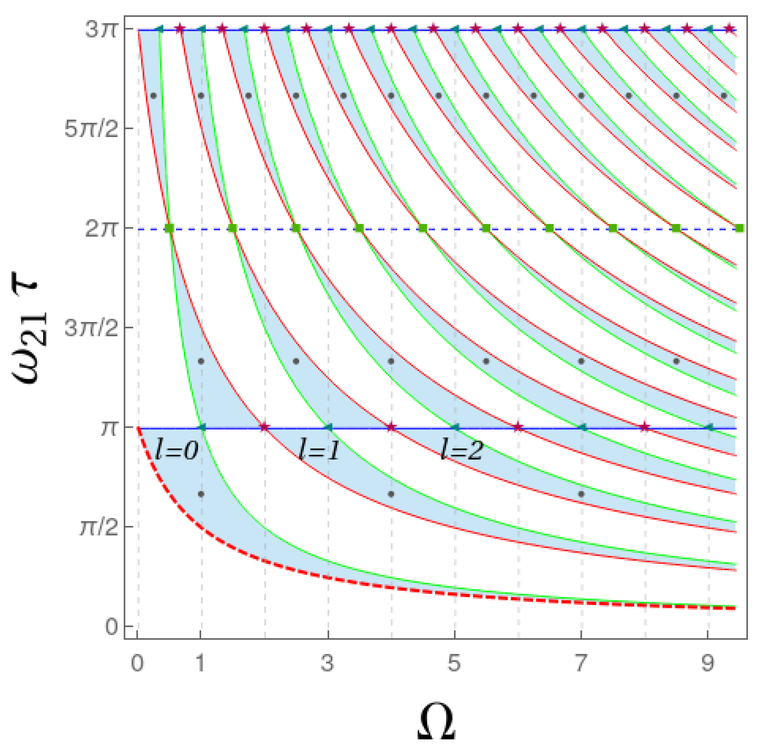
. To get insight into the set of values allowed by this restriction, we identify the elements that pertain to Family II in the phase diagram corresponding to the space determined by the dimensionless orthogonality time
and the ratio
. This diagram is shown in
Figure 1, and the permitted values—numerically calculated consistently with Equation (
8) and the condition
—form the ‘zebra stripe’-like pattern depicted by the blue shaded regions,
excluding the borders. Thus, each point in the blue region represents a triad
that satisfies Equation (
8) for the corresponding values of
and
. Likewise, the points in the borders of the zebra stripes represent triads that pertain to Family I, as shown in what follows.
According to the results in
Section 2.1, for the
s of Family I-qubit, we have:
corresponds to
and is represented by the horizontal solid-blue lines in
Figure 1.
corresponds to
. By writing
, this is equivalently expressed as
represented by the red curves.
corresponds to
. With
, this amounts to
represented by solid-green curves.
For the triads in Family I-b, an analysis of the cases described below Equation (
6) shows that:
- ■
corresponds to
with
. Consequently, the points representing these triads (marked with a star symbol) are found in the intersections of the solid-blue lines with the lines (not shown in
Figure 1)
.
- ■
corresponds to
with
. The triads are therefore located at the intersections (marked with the left-triangle symbol) of the solid-blue lines with the lines (not shown)
.
- ■
corresponds to
with
. The set of coefficients are thus located at the intersections (marked with square symbol) of the dashed-blue lines with the lines (not shown)
.
The above results confirm that the borders of the blue shaded regions do indeed represent solutions in Family I. The interior of the zebra stripes, as stated above, contains those that pertain to Family II, which can be located arbitrarily near to the borders. This can be verified as follows. For simplicity, we consider the zebra stripes (labeled as
) contained in the region
of the diagram
vs.
. In
, we have that
, which, together with the condition
, implies that the denominator in Equation (
8) is a negative quantity; consequently,
gives
, which leads to the conditions
for
. By use of these inequalities and the relation
, we have
. However, the condition
implies that
, and consequently the bounds of
are tightened to
Now, by writing
and
, the inequalities (
15) are satisfied for each
l if
obtaining finally that the
lth zebra stripe in
is correspondingly delimited by the boundaries expressed in the inequalities
The lower and upper bounds in this expression correspond, respectively, to the red and green (or blue) borders seen above. Therefore, since
can be arbitrarily close to the bounds, there is a point inside the zebra stripes that approximates to the borders as much as desired. Physically, this means that there is a triad
for which the orthogonality time can be arbitrarily close to the limiting values in Equation (
17).
2.3. Orthogonality Time
From the lower bound of Equation (
17), we get the minimal orthogonality time for the
lth zebra stripe:
Taking
in Equation (
18), we get
thus
—represented by the red-dashed curve in
Figure 1—stands for the
global minimal possible amount of time required to reach orthogonality. Since
, orthogonality can be reached more quickly as the separation between the extreme levels increases. Recall, however, that this minimal time is not attainable for states in Family II, lying inside the zebra stripe; however, as discussed above, it is always possible to find a point inside the blue-shaded area corresponding to a three-level state that attains orthogonality at a time arbitrarily close to
.
The two upper bounds in Equation (
17) coincide whenever
. For
, this occurs when the separation between levels coincide, so that
and
. This equally-spaced case is indicated with the vertical dashed line
in
Figure 1 and corresponds, according to Equation (
8), to
As a particular example of this equally-spaced energy levels case, we find the
s for the equally-probable superposition, corresponding to
(represented in
Figure 1 by dark dots at the ‘center’ of each zebra stripe). From Equation (
20), we have that
must satisfy
, which leads to
The first of these values,
(corresponding to the dot inside the
zebra stripe), determines the time at which
becomes distinguishable from the initial state
for the first time, while the second,
(second point on the vertical line
), gives the time at which a second distinguishable state,
, orthogonal to
and , is reached [
34]. This is a particular example (for
) of the previously studied case of equally-weighted superpositions of
non-degenerate and equally-spaced states [
34]. Furthermore, the regular distribution of the dark dots in the middle of each zebra stripe is a consequence of a more general property, namely, that each distribution corresponding to a given
and
in stripe
periodically appears in all other stripes at the same
and
.
In
Figure 1, we observe that, for
, there exist triads of Family II that give rise to states
and
that are mutually orthogonal for
any in the interval
. For
in the region
, the allowed values of the orthogonality time are grouped into bands, whose number increases, decreasing their width, as
acquires higher values. In any case, it should be noted that
at least one solution exists for
all , meaning that a three-level system can be made to reach an orthogonal state in a finite time
, provided the expansion coefficients
, which specify the initial state preparation (
1), are adequately chosen.
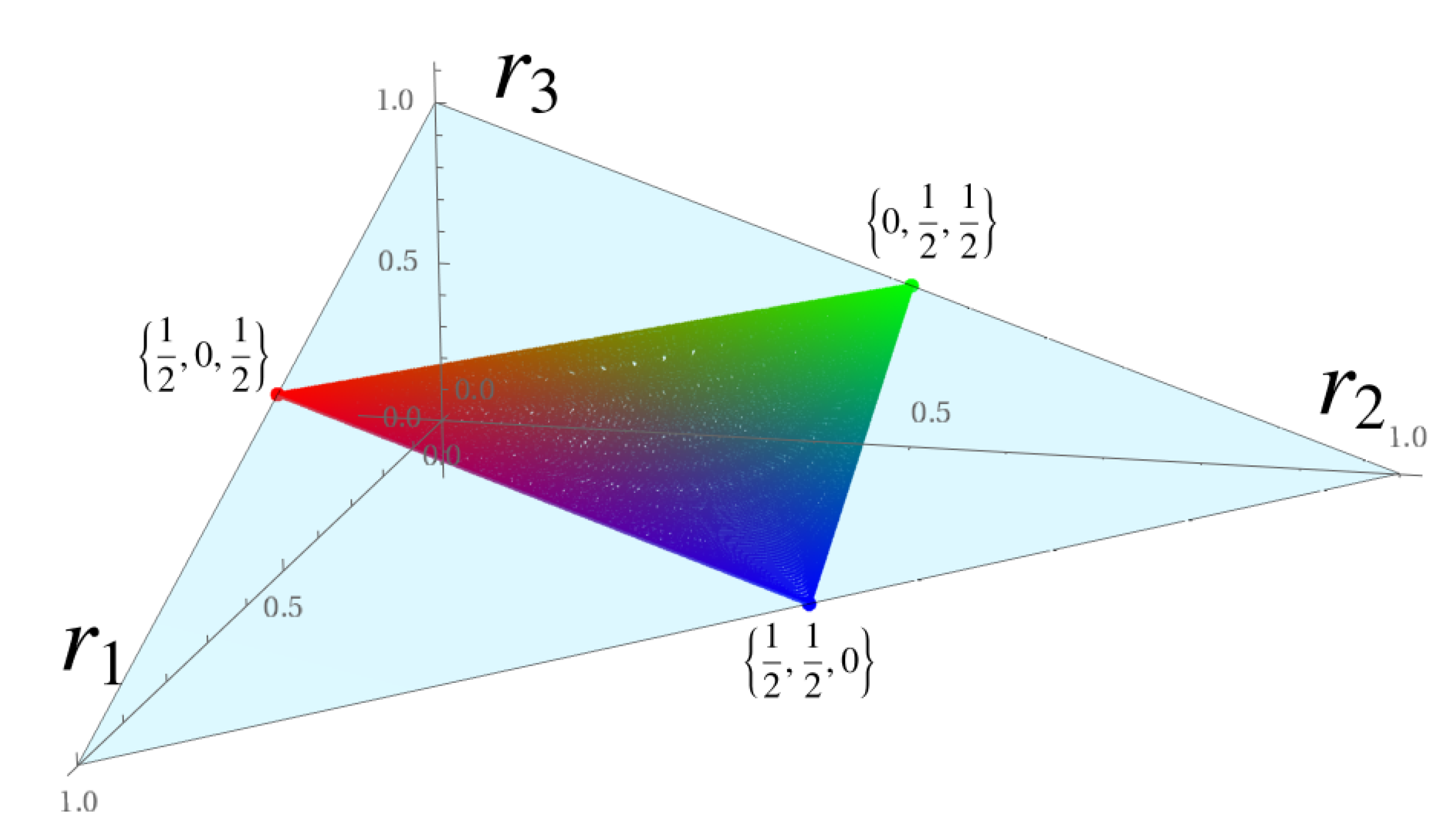
Before ending this section, and in order to gain more insight into the geometric representation of the allowed
s, we now focus on the space
and identify in it the triads for which mutually orthogonal states,
and
, exist. Such points form a subset
of the
standard 2-simplex in
, the latter defined by the points
that satisfy
and
and represented by the light-blue shaded face in
Figure 2.
, which is in itself a 2-simplex, is depicted as the colored triangle. Its vertices and edges (its boundary) correspond, respectively, to the elements of the Families I-qubit and I-b, and its interior is filled with by those
in Family II. As can be seen in the figure, these latter points do satisfy
, meaning, in particular, that for highly unbalanced superpositions of energy eigenstates the orthogonality condition cannot be met.
3. The Quantum Speed Limit
It is a well-established fact that, for given energetic resources, the orthogonality time of an initial state cannot be less than the (minimal) time imposed by the so-called quantum speed limit. The QSL establishes a natural and intrinsic time-scale of the system’s dynamics and becomes relevant when characterizing the evolution rate of the system. It is therefore the central quantity of this section, aimed at determining the quantum speed limit of the states associated to the expansion coefficients that belong to the Families I and II.
The fundamental limits on the speed at which a pure quantum state evolves towards an orthogonal one under a (time-independent) Hamiltonian have been advanced in the form of lower bounds, either in terms of the relative mean energy
(as measured from the lowest eigenvalue that contributes to (
1), say
) [
16],
or in terms of the energy dispersion [
20]
,
with
. Equations (
22a) and (
22b) are, respectively, the celebrated Margolus–Levitin (ML) and Mandestam-Tamm (MT) bounds. In [
6], Levitin and Toffoli considered the unified bound [
6]
with
denoting the quantum speed limit. They proved that only for states in an equally-weighted superposition of two energy eigenstates both bounds (ML and MT) coincide
and the quantum speed limit is attained, whereas for superpositions of three energy eigenstates the unified bound is tight, so
may be arbitrarily close, although not equal, to
. This means that for the triads
in Family I-qubit
, whereas for those in the Families I-b and II it holds that
. Our aim is thus to discern which of the two bounds, ML or MT, determines the quantum speed limit of the states (
1) specified by the elements of these latter families. We do so by analyzing the parameter
which evidently determines
as the Mandelstam–Tamm bound whenever
, as the Margolus–Levitin bound provided
and by either of them (being equal) for
.
In terms of the transition frequencies
and the coefficients
,
and
are explicitly given by
For the triads in Family I-qubit, Equation (
24) reduces to
; therefore,
, bounds (
22a) and (
22b) coincide, and it is verified that
, with
. Notice that, among the three members of Family I-qubit, the one with the lowest quantum speed limit is
(represented by the red vertex of
in
Figure 2), which gives rise to the fastest qubit
that reaches a distinguishable state at
given precisely by Equation (
19).
When all three coefficients
are nonzero, we can rewrite Equation (
24) as follows
from which
can be expressed as
This allows the realization of a quantitative analysis of the quantum speed limit of states given rise by Families I and II. For an arbitrary fixed
,
depends
explicitly on the energy separations only through the ratio
. However, for the
in Family II, the
detailed dependence of
on
becomes more intricate due to Equation (
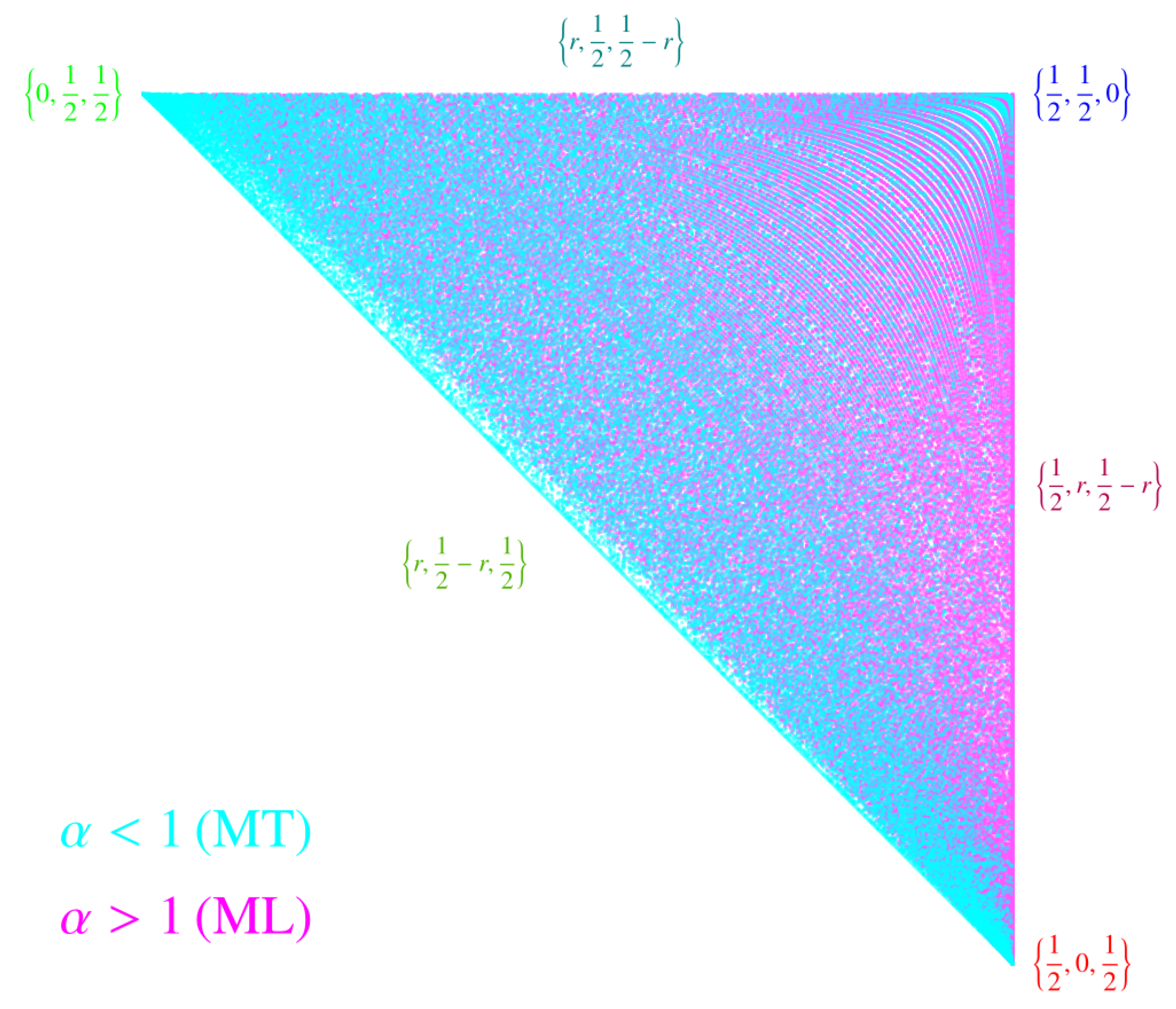
8). In
Figure 3, we show a large sample of points of the 2-simplex
that correspond to coefficients for which
, computed from (
26), is larger than 1 (the Margolus–Levitin subset
, colored in magenta), and similarly coefficients for which
(the Mandelstam–Tamm subset
, colored in cyan), for different values of
in the region
of the space
–
. The figure reveals the complex spreading of both subsets within the orthogonality simplex
, induced by the quantum speed limit; notably, there is no sharp separation between the elements of
and those of
. They appear rather mixed, although exhibiting a marked accumulation of cyan points around the edge
and the vertex
. These become diluted towards the opposite vertex
, whereas the magenta points are more dense near the vertices
and
.
The case of the triads in Family I-b, represented by the edges of
in
Figure 3, allows for a direct and simple analytical analysis for determining the corresponding range of
. With this purpose, it is convenient to analyze separately the three possible sets
as follows:
- ■
,
. These points form the edge that goes from the vertex
to
of the 2-simplex
in
Figure 2 and
Figure 3, and they correspond to
where the inequality follows from the fact that
.
- ■
,
. These points form the edge that goes from the vertex
to
in
Figure 2 and
Figure 3, and give
- ■
,
. This set of points lies along the edge that goes from the vertex
to
in
Figure 2 and
Figure 3, and their corresponding
reads
Unlike the previous cases, here, the range of
depends on the range of
. For
we have
, whereas for
we find three cases:
In this way, for a given
, the edge under consideration is divided into two segments, one cyan and one magenta, separated by the point at
. Notice that such segments are not appreciated in
Figure 3, since (as explained above) this figure considers a sample of different values of
and not a single one.
Finally,
Table 1 contains a practical summary of our main results, which completely characterize all qutrits that evolve towards an orthogonal state under a time-independent, otherwise arbitrary, Hamiltonian.
4. Summary and Final Remarks
In this paper, we completely determine and organize the set of coefficients
that provide the energy distribution and give rise to initial states (
1) that reach an orthogonal state in a finite time
, when evolving under an arbitrary time-independent Hamiltonian. A geometric organization of such coefficients is established, both in the solution diagram in the space
-
and in the 2-simplex in
. In the first case, the sets
are represented by points according to the allowed values of
and the corresponding energy-levels separation, and characteristic regions whose shape resembles zebra-like stripes emerge. The interior of each of these regions is filled with triads of Family II (
for all
i), whereas the borders correspond to triads of Family I: continuous borders represent coefficients associated to qubit states (
for some
i), and their intersections represent elements of Subfamily I-b (
for some
i,
for all
j). In the second geometric representation, the
s are organized in the central 2-simplex
, contained in the 2-simplex
of
. In this case as well, the elements in Family II fill the interior (satisfying
, whereas elements in Family I lie along the borders (edges and vertices) of
.
As is clear from the results in
Figure 1, the minimum orthogonality time
(
19) of the qubit corresponding to the triad
(dotted red line) bounds from below the orthogonality time of any other qubit or qutrit with the same energetic resources. The other qubits that attain an orthogonal state (representing equally weighted superpositions of eigenstates with energies
and
and
and
, respectively) correspond to the triads
and
and have orthogonality times that are bounded according to:
whenever
and
provided
(see Equations (
9) and (
11) with
). In the latter case, there exist qutrits whose orthogonality times may acquire any value within the interval
, whose length diminishes as
increases. Such qutrits are represented in the blue shaded region of the
zebra stripe in
Figure 1.
We furthermore analyze the quantum speed limit of the pure states given rise by the points within the 2-simplex , by constructing a map where the states whose orthogonality time is bounded by the Margolus–Levitin bound are distinguished from those for which the Mandelstam–Tamm bound limits the time evolution towards orthogonality.
Our investigation constitutes a comprehensive analysis of the exact solutions of the orthogonality condition in three-level systems. It reveals a rich underlying geometric structure and hierarchy of the allowed parameters that conform the energy distributions, while allowing for the establishment of limiting values for the orthogonality time in terms of the energy levels spacing. Further, knowledge of the expansion coefficients and their relation with provides central tools to analyze the detailed dynamics of qutrits evolving towards orthogonality and explore its relation with other relevant features, such as the amount of entanglement in composite three-level systems, which strongly depends on the sets .
We consider that our study contributes from both theoretical and practical points of view to the efforts ultimately aimed at establishing the conditions under which a N-level state transforms into a distinguishable one under a unitary transformation, irrespective of the peculiarities of the physical system. In this sense, it should be stressed that, although we assume a Hamiltonian evolution, the analysis just performed can be immediately extended to more general continuous unitary transformations , with an appropriate (-independent) generator and the corresponding evolution parameter. Our findings are thus applicable to any pure state (of single or composite systems) that can be expressed as a superposition of any three, non-degenerate, eigenvectors of and throw light onto the -distribution and the amount of evolution required to reach an orthogonal state under the transformation governed by . The results here presented thus acquire relevance in the realm of the dynamics of low-dimensional states, as well as in the field of quantum information processing, in which knowing and approximating to the fundamental limits of a quantum dynamical process improves quantum control technologies.


