Quantum Information Hidden in Quantum Fields

Abstract

We investigate a possible reduction mechanism from (bosonic) Quantum Field Theory (QFT) to Quantum Mechanics (QM), in a manner that could explain the apparent loss of degrees of freedom of the original theory in terms of quantum information in the reduced one. This reduction mechanism consists mainly of performing an ansatz on the boson field operator, which takes into account quantum foam and non-commutative geometry. Through the reduction mechanism, QFT reveals its hidden internal structure, which is a quantum network of maximally entangled multipartite states. In the end, a new approach to the quantum simulation of QFT is proposed through the use of QFT’s internal quantum network. Finally, the entropic equilibrium of fully mixed and maximally entangled states in the quantum network seems to suggest that the black hole paradox of information loss might be solved under suitable conditions.

1. Introduction

Until the 1950s, the common opinion was that quantum field theory (QFT) was just quantum mechanics (QM) plus special relativity.

But that is not the whole story, as is described in [1,2]. There, the authors mainly say that the fact that QFT was “discovered” in an attempt to extend QM to the relativistic regime is only historically accidental. Indeed, QFT is necessary and applied also in the study of condensed matter, e.g., in the case of superconductivity, superfluidity, ferromagnetism, etc.

The substantial difference between QM and QFT was understood around the 1950s [3], the Haag’s theorem [4,5,6], the breaking of spontaneous symmetry, the dynamic generation of collective modes (long range correlations). In QM the Stone-von Neumann theorem [7,8] holds: for systems with a finite number of degrees of freedom the representations of the CCRs are “unitarily equivalent”, and therefore physically equivalent. The theorem of Stone-von Neumann does not apply to QFT because the fields by their nature introduce an infinite number of degrees of freedom, and so therefore the hypothesis on which the theorem of Stone-von Neumann is based fails: in QFT there are infinitely many unitarily inequivalent representations. There are physically different “stages” or dynamic regimes.

For a review on these topics, see, for example, foundational works in [9,10,11].

Another common opinion is that QFT does not have quantum information content, differing from QM (for example, in the case of a two-levels quantum system). For an introduction to quantum information and quantum computation, see, for example, [12]. This is a very important point, of great interest to us. In fact, we don’t fully agree with this common opinion, in the sense that we believe that there is hidden quantum information in QFT. We instead agree that the quantum information content is not explicit in QFT, and, put in these terms, this can be taken as one of the main differences between QFT and QM.

Then, we maintain the following main differences between QFT and QM:

(1)

The number of degrees of freedom is infinite in QFT and finite in QM.

(2)

The representations of the canonical commutation relation (CCR) are all unitarily equivalent in QM (for the Stone-von Neumann’s theorem). Instead, QFT admits unitarily inequivalent representations (uir) of the CCR. In the case of QFT with interactions, Haag’s theorem states that the representation of the interacting fields is unitarily inequivalent to that of the free fields.

(3)

QFT does not seem to have explicit quantum information content, differing from QM.

(4)

From point 3 it follows that, while QM can be simulated directly by a quantum computer (QC), QFT cannot. The QFT must first be adjusted before being simulated, and the regulator is typically a lattice, which, however, breaks Lorentz’s invariance. For the topic of quantum simulation of QFT, see, for example [13,14].

Points 2, 3, and 4 will be discussed in more detail below.

First, however, a few questions arise (relating to points 3 and 4):

“Is there any quantum information hidden in QFT?”

Also: “How can we reduce QFT to QM in such a way that the hidden informational quantum structure, if it exists, can be revealed?”

Furthermore: “Does that quantum information structure lead to a direct simulation of the original QFT?”.

Answering these questions was the goal of this paper. So, we looked for a reduction mechanism from (bosonic) QFT to QM that could reveal QFT’s Hidden Quantum Information (HQI). We found that HQI was there and was organized in a quantum network of maximally entangled multipartite states. That was the quantum computational “skeleton” of the original QFT. Since such a “skeleton” is itself a quantum network, it seems that it is right to enter it in a one-to-one correspondence with an external QC to simulate the original QFT.

The various stages of the reduction mechanism are illustrated below, which is quite complex and requires sophisticated mathematics.

We considered a boson field operator, over which we performed an ansatz that admits an attractor in whose basin there is a flow of spatial degrees of freedom (an analogous ansatz was used for an SU(2) gauge field in [15]).

The ansatz we perform in this work corresponds to a boson translation in terms of the annihilation operator in momentum space. This defines a new vacuum and, in the case of infinite volume, the two representations are unitarily inequivalent. However, in the finite volume of the basin of the attractor, the two representations become equivalent, indicating that the (bosonic) Quantum Field Theory has been reduced to Quantum Mechanics.

Within the attractor basin it is possible to define a new metric, quantized in Planck units, that undergoes quantum fluctuations, (the quantum foam) [16,17], which induce uncertainties in the position states. The latter can be interpreted as maximally entangled qubits on the surfaces of the spheres centred at the attractor point. This is possible if an adequate non-commutative space, which is a generalization of the fuzzy sphere [18] is taken as the geometrical representation of the state space of the (maximally entangled) n-qubits states.

Within the spheres, instead, the position states are fully mixed states, and represent the spatial degrees of freedom which have been released.

The entanglement entropy of the maximally entangled states equals the total quantum entropy (the von Neumann entropy) of the fully mixed states, so that quantum information is conserved.

The study of representing qubit states by non-commutative geometry started a few years ago.

In [19] we looked for a quantum system, on a quantum (non-commutative) space, which could mimic (simulate) space-time at the Planck scale. For a review on quantum spaces, see, for example, [20], and for the relation with QFT, see [21]. The theoretical construction in [19] was developed in [22], where we found a model for quantum-computational gravity: a quantum computer on a quantum space background; namely, the fuzzy sphere.

A few words should also be spared for the important role played in this paper by the uir of the CCR in QFT. In QM, i.e., for systems with a finite number of degrees of freedom, the choice of representation is inessential to the physics, since all the irreducible representations of the canonical commutation relations (CCR) are each unitarily equivalent: this is the content of the Stone-von Neumann theorem. Thus, the choice of a particular representation in which to work, reduces to a pure matter of convenience. The situation changes drastically when we consider systems with an infinite number of degrees of freedom. This is the case of QFT, where systems with a very large number of degrees of freedom are considered. In contrast to what happens in QM, the von Neumann theorem does not hold in QFT, and the choice of a particular representation of the field algebra can have a physical meaning. From a mathematical point of view, this fact is due to the existence in QFT of unitarily inequivalent representations (uir) of the CCR (in the infinite volume or thermodynamic limit). The two particularly important cases of linear transformations are the boson translation [2,9,23,24,25] and the Velatin-Bogoliubov transformation (for bosons) [26,27].

In the context of conventional approach to Quantum Field Theory, when we try to explain the interacting theories, more than one class of representations is needed. The said phenomena was observed bay Haag and sometimes is called the Haag’s no-go theorem, which states that free and interacting fields must necessarily be defined on different unitarily inequivalent Hilbert spaces.

The main problem is that when we try to construct a physical theory, by considering, e.g., the Poincare symmetry, we select just one of these classes and simply forget about the existence of others. This causes some problems, such as Haag’s no-go theorem. On the other hand, the formulation of S-Matrix is such that one can find the final state by operating S-Matrix on the initial state without taking into account the moment of interaction, regarding it as a black box. But it is the moment of interaction that all of these classes may become equally important.

The fact of ignoring the moment of interaction derives from the common attitude of the practitioners to adopt an ontology of events, instead of an ontology of processes.

In many domains of Physics, an ontology of events seems to be the only possible one, or at least the most convenient. The typical case is the scattering of particles. All that we can practically observe are the events before and after the scattering. All that happens in the meanwhile is unknowable, and the only theories we can make concern the correlations among input and output events. This way of reasoning is sufficient for many practical purposes.

Let us now discuss processes. A process is a temporal sequence of events that is ruled by some dynamical law which characterizes the process itself. This is exactly the structural content of QFT, as stressed and explained in [1,2,9], where it is clarified that the dynamics, expressed by the equations for the interacting fields (also called Heisenberg fields), defines and characterizes the theory under study and manifests itself in the observable physical fields at the level of the observations. Events are thus the manifestations of the underlying dynamics (the process).

For example, a calculation is ruled on by the implemented algorithm. An ontology of processes does not deny that observations are about events, but hold that events are explained only in terms of the underlying process, and that the descriptions of events and processes are somehow inseparable. The expression “ontology of processes” has been borrowed from information science, where it has been introduced within the context of space-temporal databases (see, for instance, Kuhn [28]). In particular, in the reduction mechanism of QFT to QM illustrated in this paper, it is extremely important to take due account of the moment of interaction; that is, to assume an ontology of processes, as we will see in Section 8 (and in the Conclusions). Avoiding doing so would lead to an internal classical computational structure of QFT, which is itself of no real help in the simulation of the latter.

Theoretical research on quantum simulation of QFT is very urgent nowadays, because it should support important experimental applications, mainly in high energy physics (HEP), and also for setting up the fundaments of theoretical computer science (TCS) [29].

The paper is organized as follows:

In Section 2, we make an ansatz on the boson field operator, take the spatial slice at constant time equal to zero, and show that the center of an open sphere of rational radius $r_n=1/n$, where n is a positive integer, of the induced topology is an attractor, through which there is a flow of degrees of freedom of the boson field.

In Section 3, we describe a new metric within the attractive basin, which is quantized in Planck length units. This metric undergoes quantum fluctuations, which are the maximum for an open sphere of unitary radius, and disappear when approaching the attractor. So, in the classical limit, the attractor would become a singularity in which all the degrees of freedom of the boson field would be lost.

In Section 4, we show that carrying out the ansatz on the boson field corresponds, in the momentum representation, to performing a boson transformation, which defines a new vacuum state. In the limit of infinite volume, the two representations are unitarily inequivalent, but in the finite volume of the attractive basin, they are equivalent. This means that in the attractive basin, the original Quantum Field Theory has shrunk to Quantum Mechanics.

In Section 5, we hypothesize that, in the presence of quantum fluctuations of the metric, the surface of a sphere of radius $r_n$, which incorporates the attractor basin, encodes quantum information (this will be formally demonstrated in Section 6 and Section 7) and that in this case there is a relationship of uncertainty between the metric and quantum information. Due to the uncertainty relation, there are some missing qubits on the sphere, corresponding to the mixed states between two spheres of radius $r_n$ and $r_{n+1}$ respectively.

In Section 6, we illustrate the origin of the quantum information encoded by the surface of the sphere that incorporates the attractor basin, which had been hypothesized in Section 5. We show that when taking into account the ansatz (in the finite volume of the basin), the quantum fluctuations of the metric induce an uncertainty in the position state, giving rise to a superposed state that can be interpreted as a qubit. Furthermore, we show that two cat position states are maximally entangled (forming a Bell state) on the surface of the sphere, while the reduced state, which is completely mixed, is inside the sphere. Since the maximum entanglement entropy (mutual information) of the Bell state is equal to the maximum von Neumann entropy of the fully mixed state, there is no loss of quantum information. Hence, we extend this result to multipartite maximally entangled states such as the Greenberger-Horne-Zeilinger (GHZ) [30] states.

In Section 7, we show that in order to have n-partite maximally entangled states on the surface of the sphere enclosing the attractor basin, such a sphere should be a (modified) fuzzy sphere with rational radius $r_n=1/n$, in the fundamental representation of SU(2) (with two elementary cells).

In fact, in the case of a usual fuzzy sphere, the latter would encode n qubits in the $N=2^n$ irreducible representation of SU(2) [22], each one of the N cells encoding a string of n bits, and such geometrical representation would be that of a separable n-qubits state. In the case of the modified fuzzy sphere, instead, the n-maximally entangled states are accommodated in two cells, each one encoding either a string ${\left|0\right.〉}^{\otimes n}$ or a string ${\left|1\right.〉}^{\otimes n}$. Furthermore, in this way the one-to-one correspondence [19] between the Bloch sphere and the usual fuzzy sphere with unitary radius in the fundamental representation of SU(2) is maintained.

In Section 8, we show that a quantum computer can simulate both free and interacting fields once the quantum fields are reduced to a quantum network.

In Section 9, we revisit our findings in what we call the quantum black hole paradigm and explore the path from QFT’s hidden quantum information to a possible solution, under appropriate conditions, to the information loss paradox of black holes.

Section 10 is devoted to the conclusions.

2. The Ansatz Over the Boson Field Operator

Let us consider the boson field operators $\widehat{\mathsf{\Phi }}\left(x\right)$ and ${\widehat{\mathsf{\Phi }}}^{†}\left(x\right)$ that obey the following commutation relations at equal times:

$$\left[\widehat{\mathsf{\Phi }}\left(x\right),{\widehat{\mathsf{\Phi }}}^{†}\left(x\text{'}\right)\right]={\delta }^3\left(\overrightarrow{x}-\overrightarrow{x}\text{'}\right) x\equiv \left(\overrightarrow{x},t\right)\overrightarrow{x}\equiv \left\{x_1,x_2,x_3\right\}t=t\text{'}$$

(1)

$\left[{\widehat{\mathsf{\Phi }}}^{{}^{†}}\left(x\right),{\widehat{\mathsf{\Phi }}}^{†}\left(x\text{'}\right)\right]=\left[\widehat{\mathsf{\Phi }}\left(x\right),\widehat{\mathsf{\Phi }}\left(x\text{'}\right)\right]=0$.

The boson fields $\widehat{\mathsf{\Phi }}\left(x\right)$ and ${\widehat{\mathsf{\Phi }}}^{†}\left(x\right)$ are the annihilation and creation operators, respectively.

$\widehat{\mathsf{\Phi }}\left(x\right)$ annihilates the vacuum state $\left|0\right.〉$: $\widehat{\mathsf{\Phi }}\left(x\right)\left|0\right.〉=0$ and ${\widehat{\mathsf{\Phi }}}^{†}\left(x\right)\widehat{\mathsf{\Phi }}\left(x\right)$ is the boson number-density operator.

Now, let us make an ansatz for $\widehat{\mathsf{\Phi }}\left(x\right)$, given in terms of the following transformation: ${\widehat{\mathsf{\Phi }}}_A\left(x\right)=\widehat{\mathsf{\Phi }}\left(x\right)+f\left(x\right)$, where the subscript “A” stands for ansatz, and $f\left(x\right)$ is given by:

$$f\left(\overrightarrow{x},t\right)=u\left(\overrightarrow{x}\right)\cdot \hspace{0.33em}{e}^{-iEt/\hslash }$$

(2)

In Equation (2) we take the spatial slice at constant time $t=0$, and we choose:

$$u\left(\overrightarrow{x}\right)=const\cdot e^{-i\frac{\lambda \left(\stackrel{\rightharpoonup }{x}\right)}{L_P}}$$

(3)

where $L_P$ is the Planck length: $L_P={\left(\frac{\hslash G}{c^3}\right)}^{1/2}\cong 1.6\times {10}^{-33}cm$.

Then, the ansatz at constant time $t=0$ takes the form:

$${\widehat{\mathsf{\Phi }}}_A\left(\overrightarrow{x}\right)=\widehat{\mathsf{\Phi }}\left(\stackrel{\rightharpoonup }{x}\right)+const\cdot e^{-i\hspace{0.17em}\frac{\lambda \left(\stackrel{\rightharpoonup }{x}\right)}{L_P}}\hspace{0.33em}$$

(4)

For future convenience, we make the following choice for the constant: $const=1/2i$.

A similar ansatz was used for the $SU(2)$ gauge fields in [15], in order to reduce a pure non abelian gauge field theory to quantum information theory on the fuzzy sphere [18].

The complete metric space $\left(R^3,d\right)$, where d is the Euclidean metric $d\left(\overrightarrow{x},\overrightarrow{x}\text{'}\right)=\left|\overrightarrow{x}-\overrightarrow{x}\text{'}\right|$ has an induced topology which is that of the open balls with rational radii $r_n=1/n$, with n a positive integer.

The open ball of radius $r_n$ centered at $\overrightarrow{x}*$ is:

$$B\left({\overrightarrow{x}}^{*}\right)=\left\{\overrightarrow{x}\in R^3\left|d({\overrightarrow{x}}^{*},\overrightarrow{x})<r_n\right.\right\}.$$

(5)

Now, let us make the following natural choice for $\lambda \left(\overrightarrow{x}\right)$:

$$\lambda \left(\overrightarrow{x}\right)=\overrightarrow{x}*e^{i\frac{\left|{\overrightarrow{x}}^{*}-\overrightarrow{x}\right|}{n{L}_P}}$$

(6)

where ${\stackrel{\rightharpoonup }{x}}^{*}$ is a fixed point for $\lambda (\stackrel{\rightharpoonup }{x})$ as it holds:

$$\lambda ({\stackrel{\rightharpoonup }{x}}^{*})={\stackrel{\rightharpoonup }{x}}^{*}$$

(7)

It is easy to check that $\lambda (\stackrel{\rightharpoonup }{x})$ continuously approaches ${\stackrel{\rightharpoonup }{x}}^{*}$ for large values of n (i.e., for smaller radius of the ball): ${\lim }_{n\to \infty }\lambda (\stackrel{\rightharpoonup }{x})={\stackrel{\rightharpoonup }{x}}^{*}$.

The fixed point ${\stackrel{\rightharpoonup }{x}}^{*}$ is an attractive fixed point for $\lambda (\stackrel{\rightharpoonup }{x})$, as it holds:

$$\left|\lambda \text{'}({\stackrel{\rightharpoonup }{x}}^{*})\right|<1$$

(8)

where: $\lambda \text{'}\left({\stackrel{\rightharpoonup }{x}}^{*}\right)\equiv \frac{d}{dx}\lambda \left(\stackrel{\rightharpoonup }{x}\right)\left|{}_{\stackrel{\rightharpoonup }{x}={\stackrel{\rightharpoonup }{x}}^{*}}\right.$.

The fixed point ${\stackrel{\rightharpoonup }{x}}^{*}$ is then a particular kind of attractor for the dynamical system described by this theory.

Furthermore, it holds:

$$\left|\lambda \text{'}(\stackrel{\rightharpoonup }{x})\right|<1$$

(9)

for all $\stackrel{\rightharpoonup }{x}\in B_{r_n}\left({\stackrel{\rightharpoonup }{x}}^{*}\right)$, which is equivalent to say that $\lambda (\stackrel{\rightharpoonup }{x})$ is a contraction map in the attraction basin of ${\stackrel{\rightharpoonup }{x}}^{*}$; that is, it satisfies the Lipschitz condition [31].

Then, it holds:

$$d\left(\lambda \left(\stackrel{\rightharpoonup }{x}\right),\hspace{0.17em}\lambda \left(\stackrel{\rightharpoonup }{x}\text{'}\right)\right)\le \hspace{0.17em}\hspace{0.17em}q\hspace{0.17em}d\left(\stackrel{\rightharpoonup }{x},\hspace{0.17em}\stackrel{\rightharpoonup }{x}\text{'}\right)$$

(10)

with $\hspace{0.17em}q\in \left(0,1\right)$ for every $\stackrel{\rightharpoonup }{x},\stackrel{\rightharpoonup }{x}\text{'}\in B_{r_n}\left({\stackrel{\rightharpoonup }{x}}^{*}\right)$.

3. The Ansatz and the Quantum Foam

It should be noted that the choice Equation (6) for $\lambda (\stackrel{\rightharpoonup }{x})$ implies that we are considering a discrete space background quantized in Planck length units $L_n=n{L}_P$, with $n\in Z^{+}$.

In the classical limit $L_P\to 0$ we have: $\lambda (\stackrel{\rightharpoonup }{x})\to \infty$, ${\widehat{\mathsf{\Phi }}}_A\left(\overrightarrow{x}\right)\to 0$.

Then, the new metric inside the basin of the attractor is:

$$g{}_n\left(\stackrel{\rightharpoonup }{x},\overrightarrow{x}\text{'}\right)=\frac{d\left(\overrightarrow{x},\overrightarrow{x}\text{'}\right)}{n{L}_p}=\frac{\left|\overrightarrow{x}-\overrightarrow{x}\text{'}\right|}{n{L}_p}, n\in Z^{+}$$

(11)

The function $\lambda (\stackrel{\rightharpoonup }{x})$ in Equation (6) can be rewritten as:

$$\lambda \left(\overrightarrow{x}\right)=\overrightarrow{x}*\exp \left[i{g}_n\left({\overrightarrow{x}}^{*},\overrightarrow{x}\right)\right]$$

(12)

The absolute value of the variation of $g_n$ with respect to $n$ is:

$$\left|\Delta g_n\right|=\frac{1}{n^2}$$

(13)

and the quantum fluctuations of the metric $g_n$ are:

$$\Delta {(g)}_n=\frac{\left|\Delta g_n\right|}{g_n}=\frac{1}{n}$$

(14)

Let us consider the Wheeler relation [16] of the quantum foam, that is the quantum fluctuations of the metric $\delta {\left(g\right)}_{ij}$ $(i,j=1,2,3)$:

$$\Delta {\left(g\right)}_{ij}=\frac{\Delta g_{ij}}{g_{ij}}=\frac{L_p}{L}$$

(15)

The maximal fluctuation occurs for $L=L_P$, that is at the Planck scale:

$$\Delta {\left(g\right)}_{ij}=1, \Delta g_{ij}=g_{ij}$$

(16)

The Wheeler relation was extended to the case of a quantum de Sitter space-time [32], which is discretized by spatial slices: $t_n=n{t}_P$, where $t_P$ is the Planck time: $t_P={\left(\frac{\hslash G}{c^5}\right)}^{1/2}\cong 5.3\times {10}^{-44}\sec$. In that context, the Wheeler relation takes the form:

$$\Delta {{\left(g\right)}_{ij}}_n=\frac{\Delta g_{ij}{}_n}{g_{i{j}_n}}=\frac{L_p}{L{}_n}$$

(17)

where $L_n$ is the proper length:

$$L_n=c{t}_n=cn{t}_P=n{L}_P, n\in Z^{+}$$

(18)

For $n=1$ we recover the maximal fluctuation of the metric as in Equation (16): $\Delta {\left(g\right)}_{ij}{}_{n=1}=1$.

In the limit $n\to \infty$, the fluctuations of the metric tend to zero: ${\lim }_{n\to \infty }\Delta {\left(g\right)}_n=0$. From Equations (17) and (18), it follows that the values of the rational radii of the balls can be identified with the quantum fluctuations of the metric:

$$\Delta {(g)}_n=1/n=r_n$$

(19)

The maximal fluctuation occurs for $n=1$, which corresponds to the maximal radius of the attractor basin. Instead, very close to the attractor point ${\stackrel{\rightharpoonup }{x}}^{*}$ (the centre of the basin)—that is, for $n\to \infty$, the fluctuations of the metric vanish $\Delta {\left(g\right)}_n\to 0$. This suggests that in absence of the quantum fluctuations of the metric, in the classical limit, the attractor would become a singularity where all the degrees of freedom of the boson field would be lost.

4. From QFT to QM

In absence of the ansatz, the operator $\widehat{\mathsf{\Phi }}\left(\overrightarrow{x}\right)$ annihilates the vacuum $\left|0\right.〉$:

$$\widehat{\mathsf{\Phi }}\left(\overrightarrow{x}\right)\left|0\right.〉=0,$$

(20)

The number operator is:

$$N={\displaystyle \int d^3\stackrel{\rightharpoonup }{x}\hspace{0.17em}\hspace{0.17em}\mathsf{\Phi }{\left(\stackrel{\rightharpoonup }{x}\right)}^{†}}\hspace{0.17em}\mathsf{\Phi }\left(\stackrel{\rightharpoonup }{x}\right)$$

(21)

and the v.e.v. of the number operator is zero:

$$\left.〈0\right|N\left|0\right.〉=0,$$

(22)

meaning that there are no particles in the vacuum state $\left|0\right.〉$.

In the $\overrightarrow{k}$-momentum space representation, the annihilation and creation operators $a\left(\overrightarrow{k}\right)$ and $a^{†}\left(\overrightarrow{k}\right)$ are given in terms of the fields operators $\widehat{\mathsf{\Phi }}\left(\overrightarrow{x}\right)$ and ${\widehat{\mathsf{\Phi }}}^{†}\left(x\right)$ respectively:

$$a\left(\overrightarrow{k}\right)=\frac{1}{L^{3/2}}{\displaystyle \int d\overrightarrow{x}\hspace{0.17em}\mathsf{\Phi }\left(\overrightarrow{x}\right)\hspace{0.17em}}{e}^{-i\overrightarrow{k}\cdot \overrightarrow{x}/\hslash }$$

(23)

$a^{†}\left(\overrightarrow{k}\right)=\frac{1}{L^{3/2}}{\displaystyle \int d\overrightarrow{x}\hspace{0.17em}{\mathsf{\Phi }}^{†}\left(\overrightarrow{x}\right)\hspace{0.17em}}{e}^{i\overrightarrow{k}\cdot \overrightarrow{x}7\hslash }$. The annihilation and creation operators $a\left(\overrightarrow{k}\right)$ and $a^{†}\left(\overrightarrow{k}\right)$ satisfy the canonical commutation relations:

$$\left[a\left(\overrightarrow{k}\right),a^{†}\left(\overrightarrow{k}\text{'}\right)\right]={\delta }^3\left(\overrightarrow{k}-\overrightarrow{k}\text{'}\right)$$

(24)

$\left[a\left(\overrightarrow{k}\right),a\left(\overrightarrow{k}\text{'}\right)\right]=0$, $\left[a^{†}\left(\overrightarrow{k}\right),a^{†}\left(\overrightarrow{k}\text{'}\right)\right]=0$, By defining:

$$N_A={\displaystyle \int d^3\stackrel{\rightharpoonup }{x}\hspace{0.17em}\hspace{0.17em}{\mathsf{\Phi }}_A{\left(\stackrel{\rightharpoonup }{x}\right)}^{†}}\hspace{0.17em}{\mathsf{\Phi }}_A\left(\stackrel{\rightharpoonup }{x}\right),$$

(25)

it holds:

$$\left.〈0\right|N_A\left|0\right.〉={\left|\alpha \right|}^2=\frac{1}{4}$$

(26)

where:

$$\alpha =\frac{1}{2i}{e}^{-i\hspace{0.17em}\frac{\lambda \left(\stackrel{\rightharpoonup }{x}\right)}{L_P}}$$

(27)

which is the density of boson condensate in the vacuum state $\left|0\right.〉$ once the ansatz has been performed.

Performing the ansatz corresponds, in the momentum $\overrightarrow{k}$-representation, to performing the boson transformation [2,9,23] for each mode $\overrightarrow{k}$:

$$a_k\to a_k\left(\theta \right)=a_k+{\theta }_k {\theta }_k\in C$$

(28)

where, in the case of homogeneous condensation, it is:

$${\theta }_k=-\frac{1}{2i} \forall \overrightarrow{k}$$

(29)

We define the new vacuum:

$$a_k\left(\vartheta \right)\left|0\left(\vartheta \right)\right.〉=0 \forall \overrightarrow{k}$$

(30)

The number of quanta with momentum $\overrightarrow{k}$ is:

$$〈\left.0\left(\vartheta \right)\right|a_k^{{}^{†}}{a}_k\left|0\left(\vartheta \right)〉\right.={\left|{\vartheta }_k\right|}^2=\frac{1}{4}$$

(31)

The generator of the boson transformation Equation (28) is a unitary operator U:

$$a_k\left(\theta \right)=U\left(\vartheta \right)a_k{U}^{-1}\left(\vartheta \right)$$

(32)

where:

$$U\left(\theta \right)=\exp \left[iG\left(\vartheta \right)\right], G\left(\theta \right)=-i{\displaystyle \int d^3}k\left({\vartheta }_k{}^{*}{a}_k-{\vartheta }_k{a}_k^{†}\right)$$

(33)

is called the displacement operator [2,9,33]. Then the new vacuum is:

$$\left|0\left(\vartheta \right)\right.〉=\exp \left[-\frac{1}{2}{\displaystyle \int d^{3}k{\left|{\vartheta }_k\right|}^2}\right]\exp \left[-{\displaystyle \int d^{3}k{\vartheta }_k{a}_k^{†}}\right]\left|0\right.〉$$

(34)

The scalar product of the two vacua is given by:

$$〈0|0\left(\vartheta \right)〉=\exp \left[-\frac{1}{2}{\displaystyle \int d^{3}k{\left|{\vartheta }_k\right|}^2}\right]$$

(35)

Now, let us consider, for example, the case of a homogeneous condensation; namely, ${\theta }_k=\vartheta \delta \left(k\right)$ [1].

We have:

$$〈0|0\left(\vartheta \right)〉=\exp \left[-\frac{1}{2}{\vartheta }^2\delta \left(k\right)\left|{}_{k=0}\right.\right]=\exp \left[-\frac{1}{2}{\vartheta }^2{\left(2\pi \right)}^{-3}V\right]$$

(36)

In the infinite volume limit $V\to \infty$ the exponential tends to zero, and the two vacuum states are orthogonal:

$$〈0|0\left(\vartheta \right)〉=0.$$

(37)

This means that the two representations are unitarily inequivalent. While this fact is admissible in QFT, it is forbidden in QM by the Stone-von Neumann theorem [7,8].

In our case, we are considering a finite spatial volume, which is the basin of the attractor; that is, the open ball of radius $r_n=1/n$, centered at ${\stackrel{\rightharpoonup }{x}}^{*}$.Then, the two vacuum states in this case are not orthogonal:

$${〈0|0\left(\vartheta \right)〉}_A\ne 0$$

(38)

(where the subscript A indicates the ansatz) and the two representations are now equivalent.

More in detail, the volume of the ball is:

$$V=\frac{4}{3}\pi r_n^3=\frac{4}{3}\pi \frac{1}{n^3}$$

(39)

By replacing Equation (39) in (36) we get:

$${〈0|0\left(\vartheta \right)〉}_n=\exp \left|-\frac{1}{12}{\vartheta }^2{\pi }^{-2}{n}^{-3}\right|$$

(40)

There is a countable set of vacuum states ${\left|0\left(\vartheta \right)\right.〉}_n$, with $n\in Z^{+}$, each one corresponding to the volume of a ball of radius $r_n=1/n$.

5. Metric-Quantum Information Uncertainty Relation

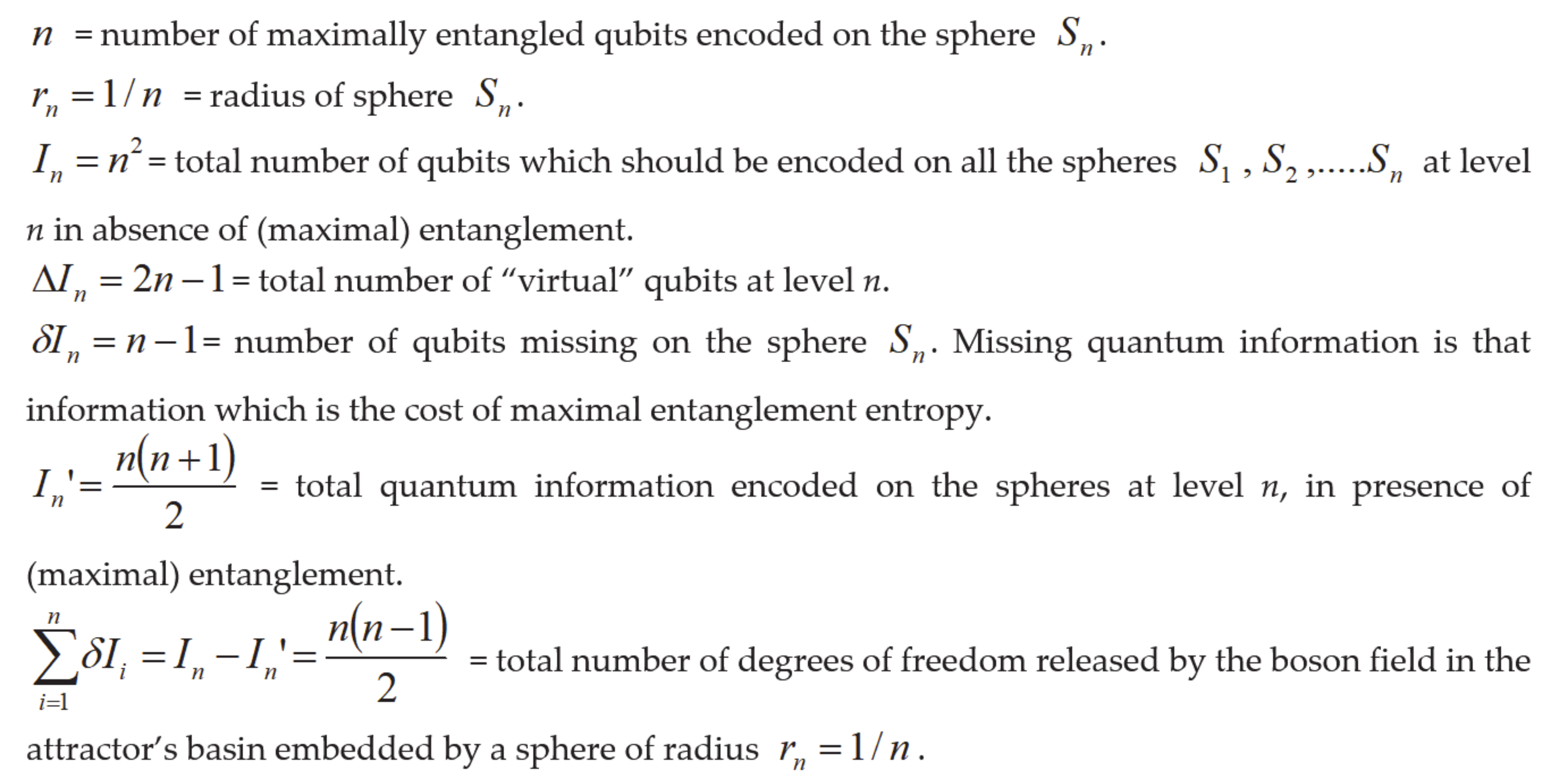
In [32] it was shown that the quantum information $I_n$ (the total number of qubits) stored by the nth cosmological horizon of a discrete quantum de Sitter space-time, with quantum fluctuations of the metric: $\Delta {(g)}_n=\frac{1}{n+1}$ was: $I_n={\left(n+1\right)}^2$ with $n\in N$. Here we assume that the quantum information encoded by the surface of a sphere $S_n$ of radius $r_n=1/n$, embedding the attractor’s basin in presence of quantum fluctuations of the metric $\Delta {(g)}_n=1/n$ is:

$$I_n=n^2$$

(41)

The variation of $I_n$ from slice $n$ to slice $n-1$ is:

$$\Delta I_n=I_n-I_{n-1}=2n-1$$

(42)

In [34] it was shown that $\Delta I_n$ is the number of the “virtual qubits” (whose occurrence is due to the quantum fluctuations of the metric), which will be transformed into real qubits by Hadamard gates at each node.

Then, within the basin of the attractor, $\Delta {(g)}_n$ and $\Delta I_n$ are linked by the uncertainty relation:

$$\Delta I_n\cdot \Delta {(g)}_n=2-\frac{1}{n}\ge 1$$

(43)

which is saturated for $n=1$.

In fact, for $n=1$ we get:

$$\Delta {(g)}_1=1=\Delta {(g)}_{MAX}=g_1, r_1=1=r_{MAX}, \Delta I_1=1=I_1=I_{MIN}$$

(44)

that is, the fluctuations of the metric get the maximal value, the maximal radius is the unit radius of the Bloch sphere, and quantum information $I_1$ is one qubit.

In what follows, we will analyze the distribution of both the “real” qubits (pure states encoded on the surface of the sphere $S_n$) and “virtual” qubits (mixed states in the interior of a sphere, for example in between sphere $S_n$ of radius $r_n=1/n$ and sphere $S_{n+1}$ of radius $r_{n+1}=1/n+1$).

If we wanted to rebuild the quantum fluctuations of the metric $\Delta {(g)}_n=1/n$ at level n from virtual quantum information, we would see that the latter is too large because of the uncertainty relation (43):

$$\Delta {\left(g\right)}_n\ge \frac{1}{2n-1}$$

(45)

This means that not all virtual qubits are transformed into pure states on the surface of the sphere $S_n$, but some of them are transformed into mixed states below the surface.

Then we redefine the virtual quantum information as:

$$\Delta I_n\text{'}=\Delta I_n-\delta I_n$$

(46)

where:

$$\delta I_n=n-1$$

(47)

This is the number of degrees of freedom released by the quantum field at level $n$. The remaining $n$ states are $n$ qubits at each level $n$.

Note that the redundancy of $\Delta I_n$ is peculiar of the uncertainty relation (43), which instead was not valid in [34].

Now, the information $\delta I_n$ is not really lost, but simply transformed into the entanglement entropy of pure n-multipartite states maximally entangled at every level n, as we will see in Section 6.

More in detail, we will consider n-maximally entangled states: for $n=2$, the Bell states:

${\left|{\mathsf{\Phi }}^{+}\right.〉}_{AB}=\frac{1}{\sqrt{2}}\left({\left|0\right.〉}_A\otimes {\left|0\right.〉}_B+{\left|1\right.〉}_A\otimes {\left|1\right.〉}_B\right)$ and for $n>2$, the Greenberger–Horne–Zeilinger (GHZ) [30] states:

$${\left|GHZ\right.〉}_n=\frac{1}{\sqrt{2}}\left({\left|0\right.〉}^{\otimes n}+{\left|1\right.〉}^{\otimes n}\right)n>2.$$

At this point one might argue that transforming quantum information into entropy means that there is a loss of quantum information, which is forbidden by the conservation principle of quantum information. But this not the case, because entanglement entropy is strictly related to mutual quantum information. This relationship, which is fairly well known, will, however, be briefly discussed in Section 6.

However, it must be said that the transformation of missing information into mutual information is a process that can take place as long as the discrete quantum structure of space holds up, since in the classical limit this is no longer possible. In fact, we would get:

$$\Delta {(g)}_n\to 0r_n\to 0\Delta I_n\to \infty , \delta I_n\to \infty n\to \infty$$

(48)

which means that very close to the attractor, where the quantum fluctuation of the metric vanish (the quantum structure of space is lost) all the spatial degrees of freedom flow inside the singularity.

In summary, at each level $n$, there are are $2n-1$ virtual states that should be transformed into qubits. However, because of the uncertainty relation (43) there are $n-1$ missing qubits on the sphere $S_n$, corresponding to the $n-1$ mixed states in between sphere $S_n$ and sphere $S_{n+1}$. The remaining $n$ qubits are maximally entangled, with maximal entanglement entropy, which is 1, equating the quantum entropy of the fully mixed states.

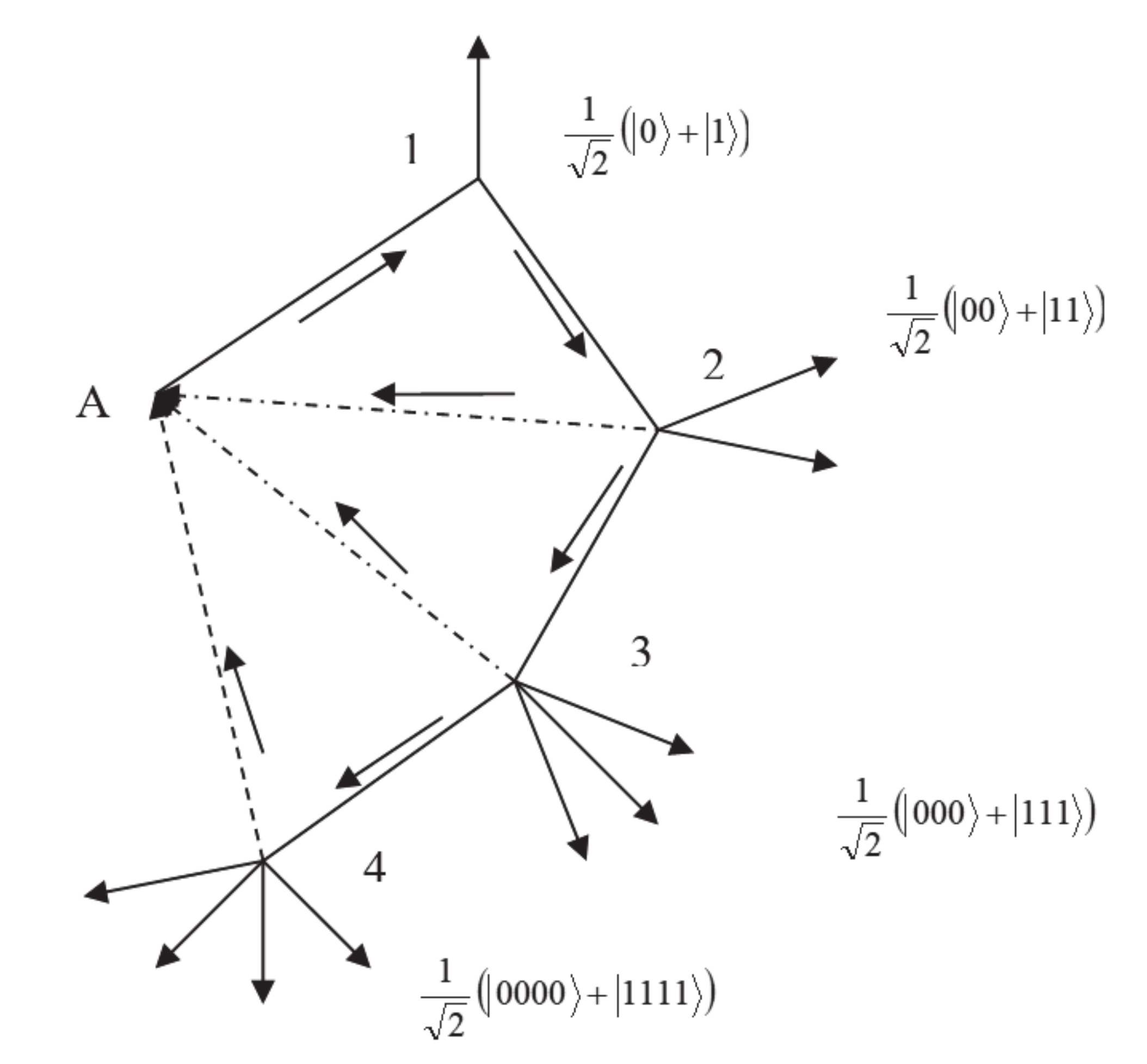
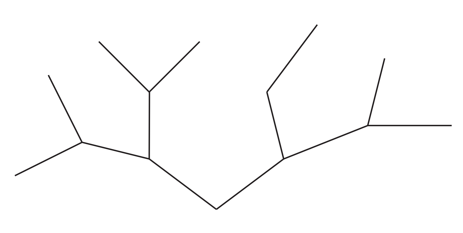
The whole picture described so far can be formalized by a quantum network, which we call the “Hidden Quantum Network” (HQN) of (bosonic) QFT, with the following rules:

• There are $n$ nodes, with $n=1,2,3\dots \mathrm{.}$
• Each node $n$ is connected to the previous node $n-1$, to the next node $n+1$ and to infinity (the attractor A) by $2n-1$ links. The latter represent the $2n-1$ virtual qubits induced by the quantum fluctuations of the metric.
• Of the $2n-1$ links, $n$ of them are going from node $n-1$ to node $n$ and from node $n$ to node $n+1$. They are the $n$ virtual states which are transformed into $n$ real qubits.
• Of the $2n-1$ links, the remaining $n-1$ are the links connecting the nodes $n$ to the attractor A. They are fully mixed states.

Of course, only at node $n=1$ there are no mixed states.

5.

At each node $n$ there are $n$ outgoing arrows representing $n$ maximally entangled qubits. See Figure 1.

The dotted connecting links are fully mixed states, converging in the attractor A.

The non-dotted connecting links are virtual states.

The nodes, labeled with integers n, represent the n spherical surfaces in the attractor basin.

The free outgoing links on each node n represent n qubit states, which are maximally entangled for any n > 1.

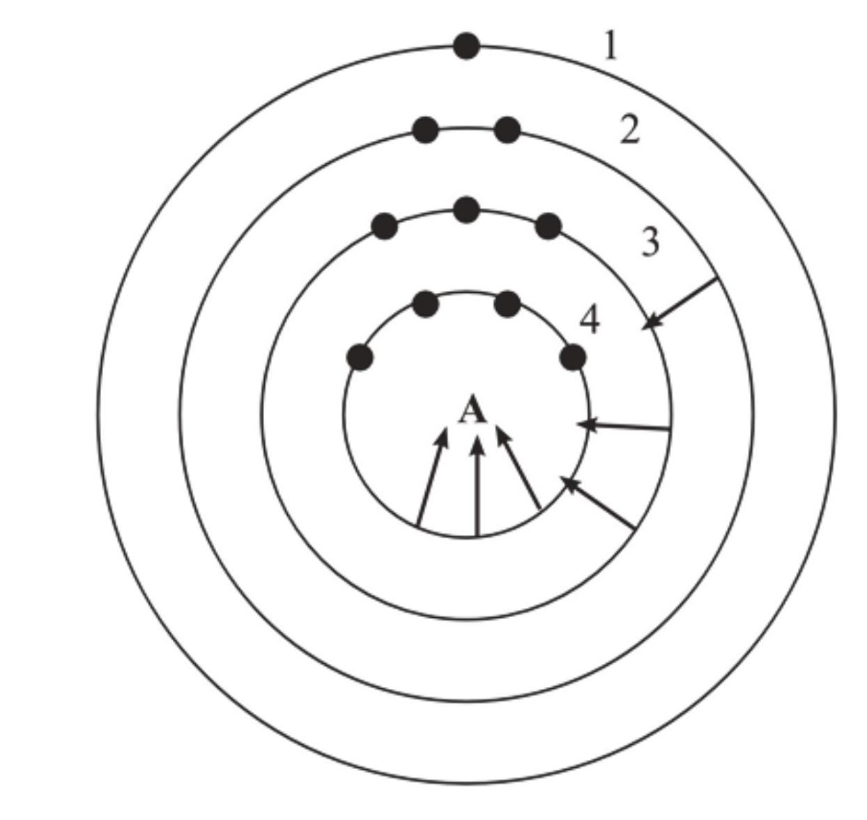
In terms of the $S_n$ spheres, the quantum network of Figure 1 can be visualized as in Figure 2.

The concentric circles, labeled by a positive integer n = 1,2,3… represent the surfaces of the n spheres centered in the attractor A.

The dots on the circles represent the maximally entangled n-qubits encoded by the nth surface.

The n − 1 arrows pointing from the nth surface to A, represent n − 1 fully mixed states.

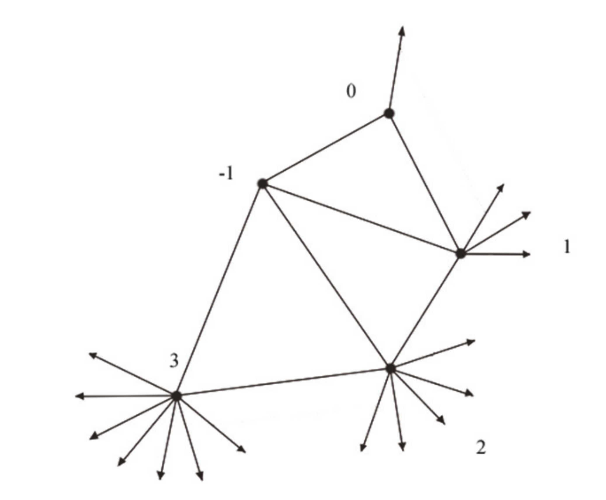
It might be worth pointing out the difference between the quantum network in Figure 1 and that described in [34], and illustrated in Figure 3, where all the virtual qubits have been transformed into real ones and have not been mixed. The quantum network of Figure 3, which illustrates the quantum information content of the inflationary era was called the “Quantum Growing Network” (QGN).

The outgoing free links are qubits.

The connecting links are virtual states.

The nodes, labeled by integers, are Hadamard gates.

For a summary, we will show Scheme A1 and

Table A1. The relevant quantities in the attractor’s basin at each level n Values of the radius of the attractor’s basin and of quantum information at each level n.

n	$r_n=1/n$	$I_n=n^2$	$\Delta I_n=2n-1$	$\delta I_n=n-1$	$I_n\text{'}=\frac{n\left(n+1\right)}{2}$	${\displaystyle \sum _{i=1}^n\delta }{I}_i=\frac{n\left(n-1\right)}{2}$
n=1	$r_1=1$	$I_1=1$	$\Delta I_n=1$	$\delta I_1=0$	$I_1\text{'}=1$
n=2	$r_2=1/2$	$I_2=4$	$\Delta I_2=3$	$\delta I_2=1$	$I_2\text{'}=3$
n=3	$r_3=1/3$	$I_3=9$	$\Delta I_3=5$	$\delta I_3=2$	$I_3\text{'}=6$	$\delta I_2+\delta I_3=3$
n=4	$r_4=1/4$	$I_4=16$	$\Delta I_4=7$	$\delta I_4=3$	$I_4\text{'}=10$	$\delta I_2+\delta I_3+\delta I_4=6$

in the Appendix A.

6. Quantum Fields and Quantum Entropy

The spatial degrees of freedom of the quantum field did flow inside the attractor’s basin, and filled it with quantum entropy. The latter is the von Neumann entropy defined as: $S\left(\rho \right)\equiv -Tr\left(\rho \lg \rho \right)$, where $\rho$ is the density operator of the quantum system:

$$\rho \equiv {\displaystyle \sum _i{p}_i\left|{\mathsf{\Psi }}_i\right.〉}\left.〈{\mathsf{\Psi }}_i\right|, \left|{\mathsf{\Psi }}_i\right.〉$$

are the quantum states, and $p_i$ are the probabilities.

A pure state is defined as $\rho =\left|\mathsf{\Psi }\right.〉\left.〈\mathsf{\Psi }\right|$.

For a pure state, it holds: $Tr{(\rho )}^2=Tr\left(\rho \right)=1$, $S\left(\rho \right)=0$, while for a generic mixed state it is:

$$Tr{(\rho )}^2<1, S\left(\rho \right)>0.$$

Let us consider now the pure quantum state $\left|\mathsf{\Psi }\right.〉$, which is the one-boson state in the position eigenstate $\left|\overrightarrow{x}\right.〉$ at position $\overrightarrow{x}$:$\left|\overrightarrow{x}\right.〉={\mathsf{\Phi }}^{†}\left(\overrightarrow{x}\right)\left|0\right.〉$. The density matrix is: $\rho =\left|\overrightarrow{x}\right.〉\left.〈\overrightarrow{x}\right|={\widehat{\mathsf{\Phi }}}^{†}\left(\overrightarrow{x}\right)\widehat{\mathsf{\Phi }}\left(\overrightarrow{x}\right)$.

We remind that ${\widehat{\mathsf{\Phi }}}^{†}\left(\overrightarrow{x}\right)\widehat{\mathsf{\Phi }}\left(\overrightarrow{x}\right)$ is the boson number-density operator: $N={\displaystyle \int {\widehat{\mathsf{\Phi }}}^{†}\left(\overrightarrow{x}\right)\widehat{\mathsf{\Phi }}\left(\overrightarrow{x}\right)}\hspace{0.33em}{d}^3\overrightarrow{x}$. The quantum entropy is zero, as it should be for pure states:

$$S\left(\stackrel{\rightharpoonup }{x}\right)\equiv Tr\left({\widehat{\mathsf{\Phi }}}^{†}\left(\overrightarrow{x}\right)\widehat{\mathsf{\Phi }}\left(\overrightarrow{x}\right)\lg \left({\widehat{\mathsf{\Phi }}}^{†}\left(\overrightarrow{x}\right)\widehat{\mathsf{\Phi }}\left(\overrightarrow{x}\right)\right)\right)=0.$$

However, when the ansatz is taken into account (in the finite volume of the basin), the quantum fluctuations of the metric $\delta g_n(\overrightarrow{x})$ induce an uncertainty $\left|\Delta {\overrightarrow{x}}_n\right.〉$ in the position state $\left|\overrightarrow{x}\right.〉$ at each level n, where $\Delta {\overrightarrow{x}}_n$ is defined as:

$$\Delta {\overrightarrow{x}}_n=L_P{\left(\frac{n}{\delta g_n\left(\overrightarrow{x}\right)}\right)}^{\frac{1}{2}}$$

(49)

The above expression of $\Delta \overrightarrow{x}$ in terms of the metric fluctuations was obtained by the use of the following relations introduced in [32]:

$$\Delta {\overrightarrow{x}}_n=\frac{L_n}{{\left(g_n\left(\overrightarrow{x}\right)\right)}^{1/2}}\left(L_n=n{L}_P\right), \frac{\delta g_n\left(\overrightarrow{x}\right)}{g_n\left(\overrightarrow{x}\right)}=\frac{1}{n}.$$

From the uncertainty relation in Equations (43) and (49), it also follows:

$$\Delta x_n=L_n\hspace{0.33em}{\left(\frac{\Delta I_n}{2n-1}\right)}^{\frac{1}{2}} (\mathrm{where} \Delta x_n=\left|\Delta {\overrightarrow{x}}_n\right|)$$

(50)

which shows the relation between the uncertainty in the position state of the boson field and the uncertainty in the quantum information at level n.

It is worth considering the particular case $n=1$ for which it holds:

$$\delta g_1=g_1=1, L_1=L_p, \Delta I_1=I_1=1$$

In this case we get, from Equation (49):

$$\Delta x_1=L_P$$

(51)

The apparently harmless result in Equation (51) is discussed in more detail in Section 9, where we show its relationship to a Planckian black hole (see also Figure 13). Here we limit ourselves to anticipating the fact that the uncertainty in the position state of the boson field is somehow responsible for quantum cosmological models such as Sitter’s quantum Euclidean universe [32].

We can redefine the position state $\left|\overrightarrow{x}\right.〉$ as the superposed state:

$$\left|\overrightarrow{x}\right.〉\to \frac{1}{\sqrt{2}}\left(\left|\overrightarrow{x}\right.〉\pm \left|\Delta \overrightarrow{x}\right.〉\right)\equiv {\left|\mathsf{\Psi }\right.〉}_A$$

(52)

(In Equation (52) the subscript “n” has been omitted).

Consider now a second position state $\left|\overrightarrow{x}\text{'}\right.〉$, which can also be redefined as:

$$\left|\overrightarrow{x}\text{'}\right.〉\to \frac{1}{\sqrt{2}}\left(\left|\overrightarrow{x}\text{'}\right.〉\pm \left|\Delta \overrightarrow{x}\text{'}\right.〉\right)\equiv {\left|\mathsf{\Psi }\right.〉}_B$$

(53)

In the following, we will consider only the plus sign in both Equations (52) and (53) for simplicity.

Now, let us identify the position state $\left|\overrightarrow{x}\right.〉$ and its uncertainty $\left|\Delta \overrightarrow{x}\right.〉$ with the computational basis states of $C^2$, that is, with the logical bits $\left|0\right.〉$ and $\left|1\right.〉$, respectively:

$$\left|\overrightarrow{x}\right.〉\equiv \left|0\right.〉, \left|\Delta \overrightarrow{x}\right.〉\equiv \left|1\right.〉.$$

The two states in Equations (52) and (53) are then identified with the qubit cat-states, respectively:

$${\left|\mathsf{\Psi }\right.〉}_A=\frac{1}{\sqrt{2}}{\left(\left|0\right.〉+\left|1\right.〉\right)}_A, {\left|\mathsf{\Psi }\right.〉}_B=\frac{1}{\sqrt{2}}{\left(\left|0\right.〉+\left|1\right.〉\right)}_B$$

(54)

Let us consider the following three cases. The two qubits in (54) can be:

(a)

Uncorrelated

(b)

Mixed

(c)

Entangled

In case (a) their joint entropy is: $S(A,B)=2$, and their mutual entropy (mutual information, in bits), defined as $S(A:B)=S\left(A\right)+S\left(B\right)-S\left(A,B\right)$ is zero: $S(A:B)=0$.

In case (b), their joint entropy is: $S(A,B)=1$ and their mutual entropy is: $S(A:B)=1$.

In case (c) their joint entropy is zero because a Bell state is a pure state: $S(A,B)=0$, but their mutual entropy is maximal, as in this case it measures the degree of entanglement: $S(A:B)=2$.

The available information is quantum, and is limited by the Holevo bound [35].

Quantum information $I$ is the mutual quantum entropy. The quantum mutual entropy is defined as follows: If ${\rho }_{AB}$ is the joint state of two quantum systems A and B, the mutual entropy $S\left({\rho }_A:{\rho }_B\right)$ is: $I\equiv S\left({\rho }_A:{\rho }_B\right)=S\left({\rho }_A\right)+S\left(\rho {}_B\right)-S\left(\rho {}_{AB}\right)$.

The Holevo theorem [35] states that the available information $I_A$—that is, the information that can be obtained from a generalized quantum measurement (or POVM = positive operator-valued measure)—cannot exceed the mutual entropy: $I_A\le S\left({\rho }_A:{\rho }_B\right)$, the latter given in bits. We recall that the number of bits corresponding to n qubits is $2^n$.

From the above it follows:

$$I_A\equiv I_n=n, I\equiv S\left({\rho }_A:{\rho }_B\right)\ge 2^{n-1}$$

(55)

where $2^{n-1}$ is $2^n$ the number of bits corresponding to n qubits divided by 2.

Notice that for $n=2$ it holds:

$$S\left({\rho }_A:{\rho }_B\right)\ge 2$$

(56)

which is saturated for maximally entangled $n=2$ (A and $B$) states.

We conclude that for $n=2$, corresponding to the radius $r_2=\frac{1}{2}$, the bipartite system of two position cat-states is maximally entangled (case c). This is the Bell state:

$${\left|{\mathsf{\Phi }}^{+}\right.〉}_{AB}=\frac{1}{\sqrt{2}}{\left(\left|00\right.〉+\left|11\right.〉\right)}_{AB}\equiv \frac{1}{\sqrt{2}}\left(\left|\overrightarrow{x}\overrightarrow{x}\right.〉+\left|\Delta \overrightarrow{x}\Delta \overrightarrow{x}\right.〉\right)$$

(57)

The cases (a) and (b) cannot occur, as they do not satisfy Equation (55).

The bipartite entanglement entropy of a pure state ${\rho }_{AB}={\left|{\mathsf{\Phi }}^{+}\right.〉}_{AB}{}_{AB}\left.〈{\mathsf{\Phi }}^{+}\right|$, denoted by $E\left({\rho }_{AB}\right)$, is defined as the von Neumann entropy of either the reduced states, as they are of the same value: $E\left({\rho }_{AB}\right)=S\left({\rho }_A\right)=S\left({\rho }_B\right)$, where:

$$S\left({\rho }_A\right)=-Tr\left({\rho }_A\log {\rho }_A\right), {\rho }_A=T{r}_B\left({\rho }_{AB}\right).$$

If the reduced state is fully mixed, then the original pure state is maximally entangled, with maximal entanglement entropy: $E{\left({\rho }_{AB}\right)}_{Max}=1$ (in log basis 2).

In the case of maximal entanglement, then, the following relation holds between the entanglement entropy and the mutual information:

$$E{\left({\rho }_{AB}\right)}_{Max}=\frac{1}{2}S\left({\rho }_A:{\rho }_B\right)=\frac{1}{2}I$$

Although the Bell state Equation (57) is a pure state:

$${\rho }_{AB}=\left|{\mathsf{\Phi }}^{+}{}_{AB}\right.〉\left.〈{}_{AB}\mathsf{\Phi }{}^{+}\right|, S\left(A,B\right)=0,$$

(58)

the reduced state is fully mixed:

$${\rho }_A=T{r}_B{\rho }_{AB}=\frac{1}{2}\left(\left|0\right.〉\left.〈0\right|+\left|1\right.〉\left.〈1\right|\right)=\frac{1}{2}\left(\left|\overrightarrow{x}\right.〉\left.〈\overrightarrow{x}\right|+\left|\Delta \overrightarrow{x}\right.〉\left.〈\Delta \overrightarrow{x}\right|\right)=\frac{1}{2}{{\rm I}}_2.$$

(59)

Note that the reduced state of case c) is identical to the reduced state in case b).

Let us consider the metric for $n=1$. The associated quantum information is $I\equiv n=1$—that is, one qubit. The particular case $n=1$, corresponds to the maximum volume of the ball with radius $r_1=1$ and the embedding surface is the Bloch sphere; that is, the geometrical representation of the state space of one qubit. The points on the surface of the Bloch sphere are pure states, such as the cat state in Equation (54), the basis states $\left|\overrightarrow{x}\right.〉$ and $\left|\Delta \overrightarrow{x}\right.〉$ (corresponding to the north and south pole respectively), and, more generally, states like $\alpha \left|\overrightarrow{x}\right.〉+\beta \left|\Delta \stackrel{\rightharpoonup }{x}\right.〉$ with ${\left|\alpha \right|}^2+{\left|\beta \right|}^2=1$.

The points inside the Bloch sphere, instead, correspond to mixed states. The maximally mixed state in this case is:

$${\rho }_{\stackrel{\rightharpoonup }{x}\hspace{0.17em}\Delta \stackrel{\rightharpoonup }{x}}=\frac{1}{2}\left(\left|0\right.〉\left.〈0\right|+\left|1\right.〉\left.〈1\right|\right)=\frac{1}{2}\left(\left|\overrightarrow{x}\right.〉\left.〈\overrightarrow{x}\right|+\left|\Delta \overrightarrow{x}\right.〉\left.〈\Delta \overrightarrow{x}\right|\right)=\frac{1}{2}{{\rm I}}_2$$

(60)

which is the same as the reduced state in case c) for $n=2$, (two qubits maximally entangled), $r_2=1/2$.

This fact suggests that being a pure state or a mixed state in this model depends on the observer: If he/she is on the surface of the Bloch sphere $S_{r=1}$ of radius $r_1=1$, he/she would see all the states inside the Bloch sphere (for example at $r_2=1/2$) as mixed states. Instead, an observer on the surface of the sphere $S_{r=1/2}$ of radius $r_2=1/2$, will see a bipartite pure state—that is, a Bell state but will see the states inside the sphere $S_{r=1/2}$ (for example at $r_2=1/3$) as mixed states, such as:

$${\rho }_{AB}=\frac{1}{2}\left(\left|00\right.〉\left.〈00\right|+\left|11\right.〉\left.〈11\right|\right)\equiv \frac{1}{2}\left(\left|\overrightarrow{x}\overrightarrow{x}\right.〉\left.〈\overrightarrow{x}\overrightarrow{x}\right|+\left|\Delta \overrightarrow{x}\Delta \overrightarrow{x}\right.〉\left.〈\Delta \overrightarrow{x}\Delta \overrightarrow{x}\right|\right).$$

(61)

Instead, an observer on the surface of the sphere $S_{r=1/3}$ will see a maximally entangled three partite state (the GHZ state): $\left|GHZ\right.〉=\frac{1}{\sqrt{2}}\left(\left|000\right.〉+\left|111\right.〉\right)$, which is also a pure state, with: ${\rho }_{GHZ}=\left|GHZ\right.〉\left.〈GHZ\right|$, $S\left({\rho }_{GHZ}\right)=0$. and so on.

7. Maximally Entangled States on Special Fuzzy Spheres

In this section we formalize and demonstrate the assumption we made since the beginning that the n pure states are encoded by the spheres $S_n$ of rational radii $r_n=1/n$, and are maximally entangled.

To this aim, we will consider a generalized version of the fuzzy sphere with radius $r_{FS}=r_n=1/n$, in the fundamental representation $N=2$ of $SU(2)$.

Let us consider the ordinary, commutative sphere $S^2$ of radius $r$ embedded in $R^3$:

$${\displaystyle \sum _{i=1}^3{x}_i^2}=r^2$$

(62)

The fuzzy sphere is constructed replacing the algebra of polynomials on the sphere $S^2$ by the non commutative algebra of complex N × N matrices, which is obtained by quantizing the coordinates $x_i$ (i = 1, 2, 3), that is, by replacing the $x_i$ by the non-commutative coordinates $X_i$:

$$x_i\to X_i=k{J}_i$$

(63)

where the $J_i$ form the N-dimensional irreducible representation of the algebra of SU(2) satisfying the commutation relations:

$$\left[J_i,J_j\right]={\epsilon }_{ijk}{J}_k \left(i,j,k=1,2,3\right)$$

(64)

where ${\epsilon }_{ijk}$ is the three-dimensional anti-symmetric tensor, and $k$ is a parameter called the non-commutativity parameter.

In terms of the new coordinates $X_i$ defined in (63), the relation in (62) becomes:

$${\displaystyle \sum _{i=1}^3{X}_i^2}=k^2{\displaystyle \sum _{i=1}^3{J}_i^2=k^2\left(N^2-1\right)}=r^2$$

(65)

where $J^2={\displaystyle \sum _{i=1}^3{J}_i^2=N^2-1}$ is the Casimir of SU(2) in the N-dim. representation.

From Equation (65) it follows:

$$k=\frac{r}{\sqrt{N^2-1}}$$

(66)

The dimension N of the irreducible representation of SU(2), that is $N=2j+1$ is equal to the number of elementary cells of the fuzzy sphere.

In the case $N=2$ (the fundamental representation) the non-commutative coordinates $X_i$ are given in terms of the Pauli matrices ${\sigma }_i$:

$$X_i=k{\sigma }_i$$

(67)

and Equation (66) becomes:

$$k=\frac{r}{\sqrt{3}}$$

(68)

In this case, the sphere is very poorly defined as only the North and the South poles can be distinguished. However, the higher is the dimensionality N of the representation, the lower is the fuzziness. From Equation (66) it follows that $k\to 0$ for $N\to \infty$, and one recovers the classical sphere $S^2$.

The concept of the area of a fuzzy elementary cell was first introduced in [22], although it was already implicit in [18] through the introduction of the constant $K=4\pi kr$, which has the dimension of a squared length.

The area $A_N{}^{EC}$of an elementary cell of the fuzzy sphere in the N-dim. irreducible representation of SU(2) is then:

$$A_N{}^{EC}=\frac{4\pi \hspace{0.17em}{r}^2}{\sqrt{N^2-1}}$$

(69)

For $N\to \infty$ $A_N{}^{EC}\to 0$, that is, the elementary cell reduces to a point.

The total area of the fuzzy sphere is:

$$A_N{}^{FS}=N\frac{4\pi r^2}{\sqrt{N^2-1}}$$

(70)

For large N, the area of the fuzzy sphere tends to the area of the ordinary sphere:

$$A_N{}^{FS}\to A^{S^2}=4\pi r^2.$$

In the particular case of $N=2$, there are two elementary cells, each one of area:

$$A_2{}^{EC}=\frac{4\pi r^2}{\sqrt{3}}$$

(71)

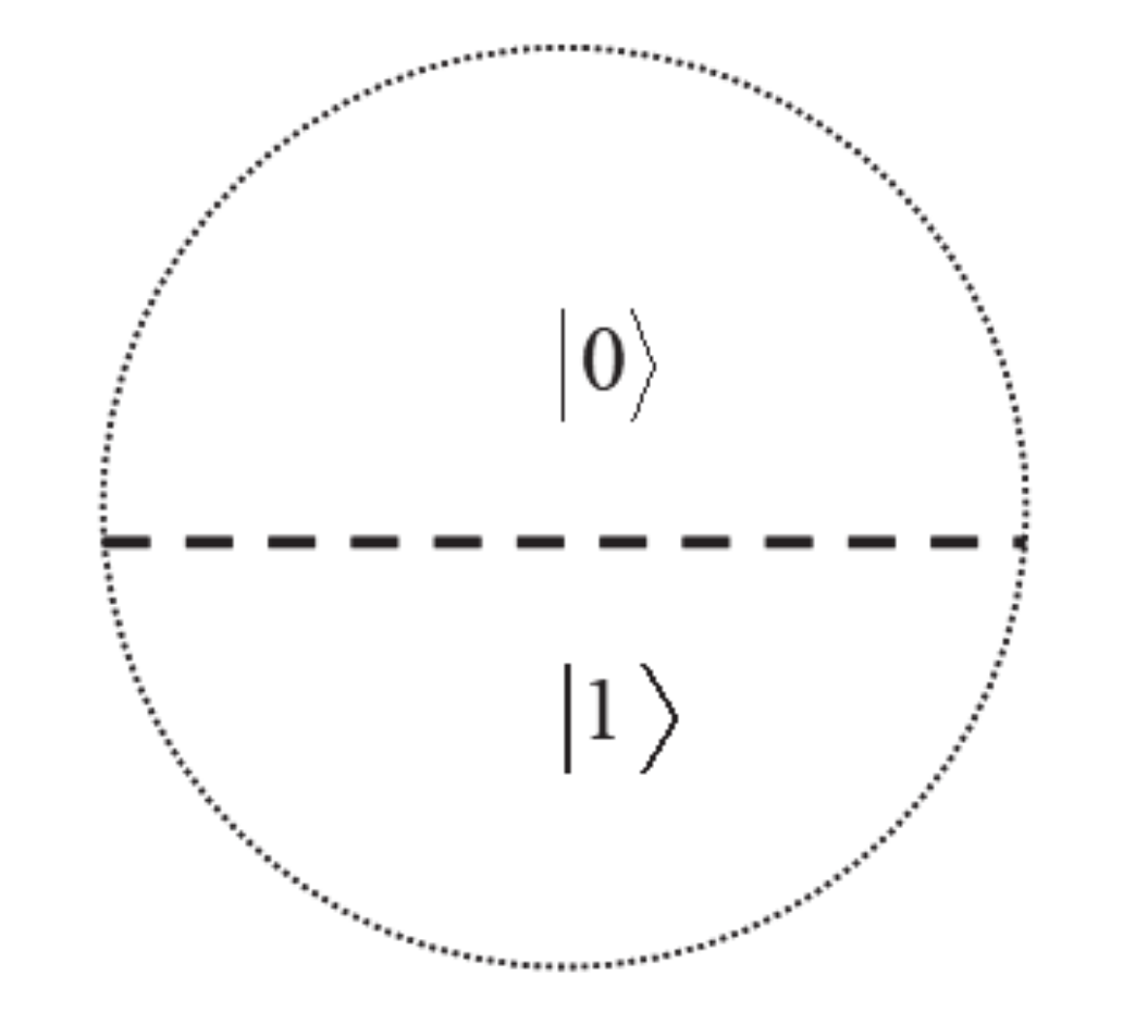
The quantum version [36,37] of the Holographic principle [38,39] is strictly related to 2-dimensional noncommutative geometry. In fact, for the case of one qubit, it was shown [19] that the geometrical representation of the qubit state space (the Bloch sphere) is in a one-to-one correspondence (a bijection) with the fuzzy sphere in the fundamental ($N=2$) representation.

For the fundamental representation $N=2$, and $r=1$ it was shown [19] that the North (N) pole $\left|0\right.〉$ and the South (S) pole $\left|1\right.〉$of the Bloch sphere are “smeared” into two elementary cells, each one of area:

$$A_2{}^{EC}=\frac{4\pi }{\sqrt{3}}$$

(72)

One cell encodes the bit $\left|0\right.〉$and the other cell encodes the bit $\left|1\right.〉$As a whole, the N = 2 fuzzy sphere encodes one qubit. See Figure 4. Some detail will be given in the Appendix B.

Two elementary cells. One cell encodes the bit $\left|0\right.〉$ and the other cell encodes the bit $\left|1\right.〉$.

As a whole, the N = 2 fuzzy sphere encodes one qubit.

In the case of many qubits, the non-commutative C*-algebra is the algebra of logic quantum gates, which are $N\times N$unitary matrices, where $N=2^n$, and $n$ is the number of qubits. For more technical details, see Appendix B.

However, the one-to-one correspondence between the fuzzy sphere and the Bloch sphere is lost for $n>1$.

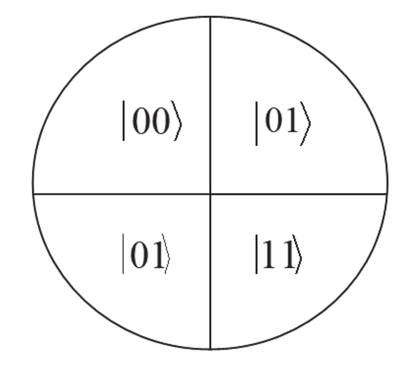
In fact, let us consider, for example the case of two qubits, $n=2$. The fuzzy sphere is in the N = 4-dim. irreducible representation of $SU\left(2\right)$ and the number of cells is $N=4$. For a unit radius, the area of an elementary cell is:

$$A_3{}^{EC}=\frac{4\pi }{\sqrt{15}}$$

(73)

Each cell encodes one of the 4 strings of $n=2$ bits: $\left|00\right.〉$, $\left|01\right.〉$, $\left|10\right.〉$, $\left|11\right.〉$, which is the geometrical representation of the state space of a separable two-qubits state. See Figure 5.

Four elementary cells. Each cell encodes a 2-bits string. As a whole, the N = 4 fuzzy sphere encodes a separable 2-qubits state.

The one-to-one correspondence with the Bloch sphere might be recovered by setting the representation $N=2$ (two cells) and considering only two strings: $\left|00\right.〉={\left(\begin{array}{c}1\\ 0\end{array}\right)}^{\otimes 2}$and $\left|11\right.〉={\left(\begin{array}{c}0\\ 1\end{array}\right)}^{\otimes 2}$.

In this way, we still have the bijection:

$$N\leftrightarrow \left|00\right.〉 S\leftrightarrow \left|11\right.〉$$

where N and S stand for North pole and South pole respectively.

The fuzzy sphere for $N=2$ will then encode the Bell state: $\left|{\mathsf{\Phi }}^{+}\right.〉=\frac{1}{\sqrt{2}}\left(\left|00\right.〉+\left|11\right.〉\right)$. See Figure 6.

To recover the one-to-one correspondence with the Bloch sphere, it will be necessary to slightly modify the definition of the area of the fuzzy elementary cells. To this purpose, we will take the radius of the fuzzy sphere, to be the radius of the sphere $S_n$ of rational radius $r_n=1/n$.

The non-commutativity parameter in Equation (66) becomes:

$$k\text{'}=\frac{1}{n\sqrt{N^2-1}}$$

(74)

In this case, the fuzzy sphere will be called “special fuzzy sphere” for any N.

We see that, once the dimension N of the irreducible representation of SU(2) is fixed, k’ depends on n. For $n\to \infty$, $k\text{'}\to 0$, and even in the case of the fundamental representation $N=2$, commutative geometry is recovered.

For $n=1$ we recover the usual fuzzy sphere, as it is: $k\text{'}=k$.

The area of the elementary cell (69) becomes:

$$A_{N,n}{}^{EC}=\frac{4\pi }{n^2\sqrt{N^2-1}}$$

(75)

For simplicity, let’s set $N=2$. Equation (75) becomes:

$$A_{N=2,n}{}^{EC}=\frac{4\pi }{n^2\sqrt{3}}$$

(76)

More details are given in the Appendix B.

Two elementary cells. One cell encodes the string $\left|00\right.〉$ and the other cell encodes the string $\left|11\right.〉$.

As a whole, the N = 2, n = 2 special fuzzy sphere encodes the Bell state $\left|{\mathsf{\Phi }}^{+}\right.〉$.

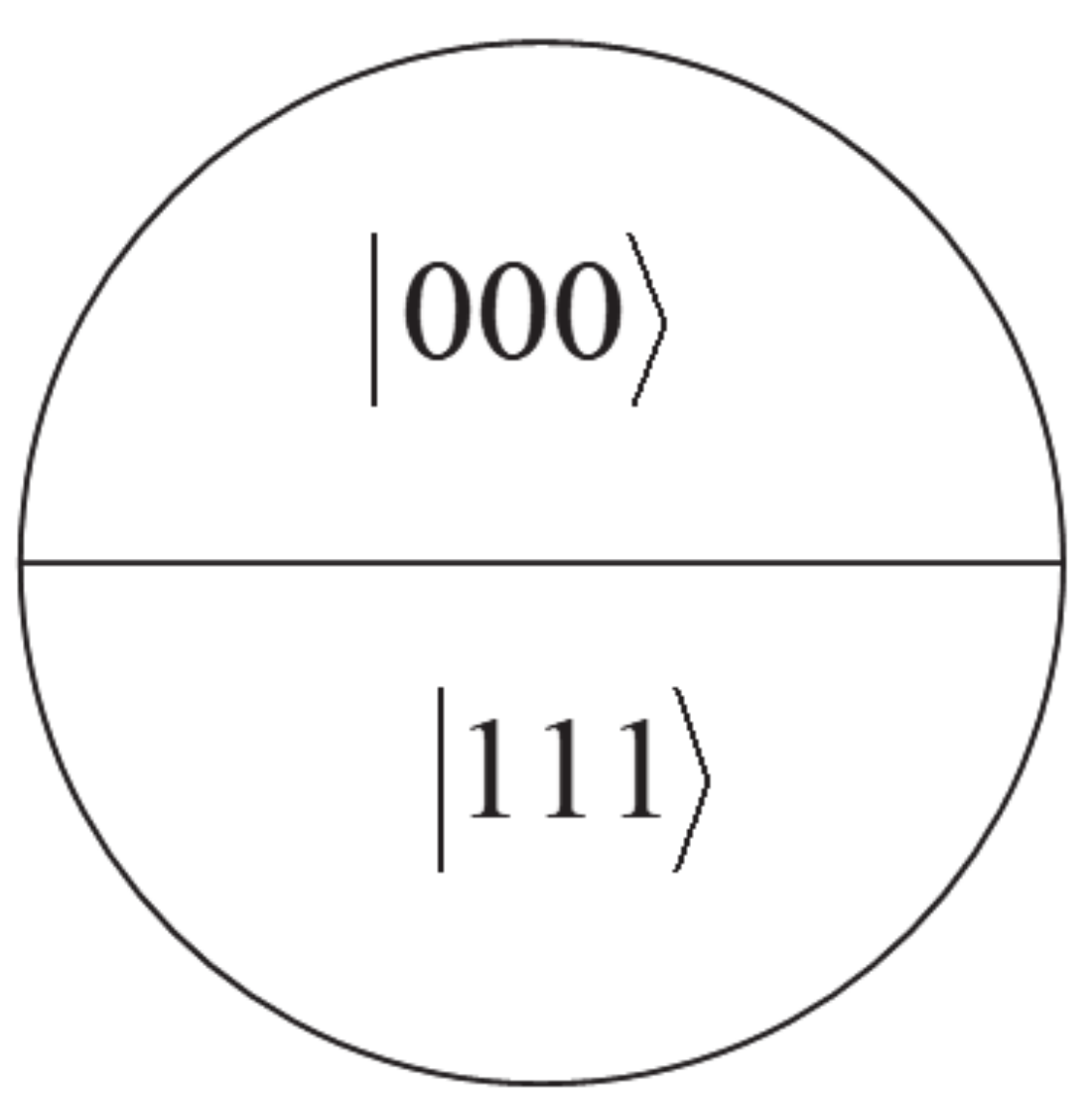
The special fuzzy sphere for $N=2, n=3$ encodes the (maximally entangled) ${\left|GHZ\right.〉}_3$ state: ${\left|GHZ\right.〉}_3=\frac{1}{\sqrt{2}}\left(\left|000\right.〉+\left|111\right.〉\right)$. More details are given in the Appendix B. See Figure 7.

Two elementary cells, each one encoding a 3-bit string. One cell encodes the string $\left|000\right.〉$, and the other cell encodes the string $\left|111\right.〉$. As a whole the N = 2, n = 3 fuzzy sphere encodes the GHZ state ${\left|GHZ\right.〉}_3$, In the same way, for $N=2, n=4$ the special fuzzy sphere will encode the (maximally entangled) ${\left|GHZ\right.〉}_4$ state: ${\left|GHZ\right.〉}_4=\frac{1}{\sqrt{2}}\left(\left|0000\right.〉+\left|1111\right.〉\right)$, and so on.

In general, the $N=2, n$ special fuzzy sphere with radius $r_n=1/n$ will encode the ${\left|GHZ\right.〉}_n$ state: ${\left|GHZ\right.〉}_n=\frac{1}{\sqrt{2}}\left({\left|0\right.〉}^{\otimes n}+{\left|1\right.〉}^{\otimes n}\right)$.

See Appendix B for more details.

8. Quantum Simulation of QFT: A New Approach

In this section, we propose a new theoretical approach to the topic of the quantum simulation of QFT, in light of the arguments discussed so far.

As is well known, quantum simulation is needed since Feynman [40] showed that a classical computer would experience an exponential slowdown when simulating quantum phenomena, while a quantum computer would not.

Then Deutsch [41] described a universal quantum computer, and Lloyd [42] showed that a standard quantum computer can be programmed to simulate any local quantum system efficiently.

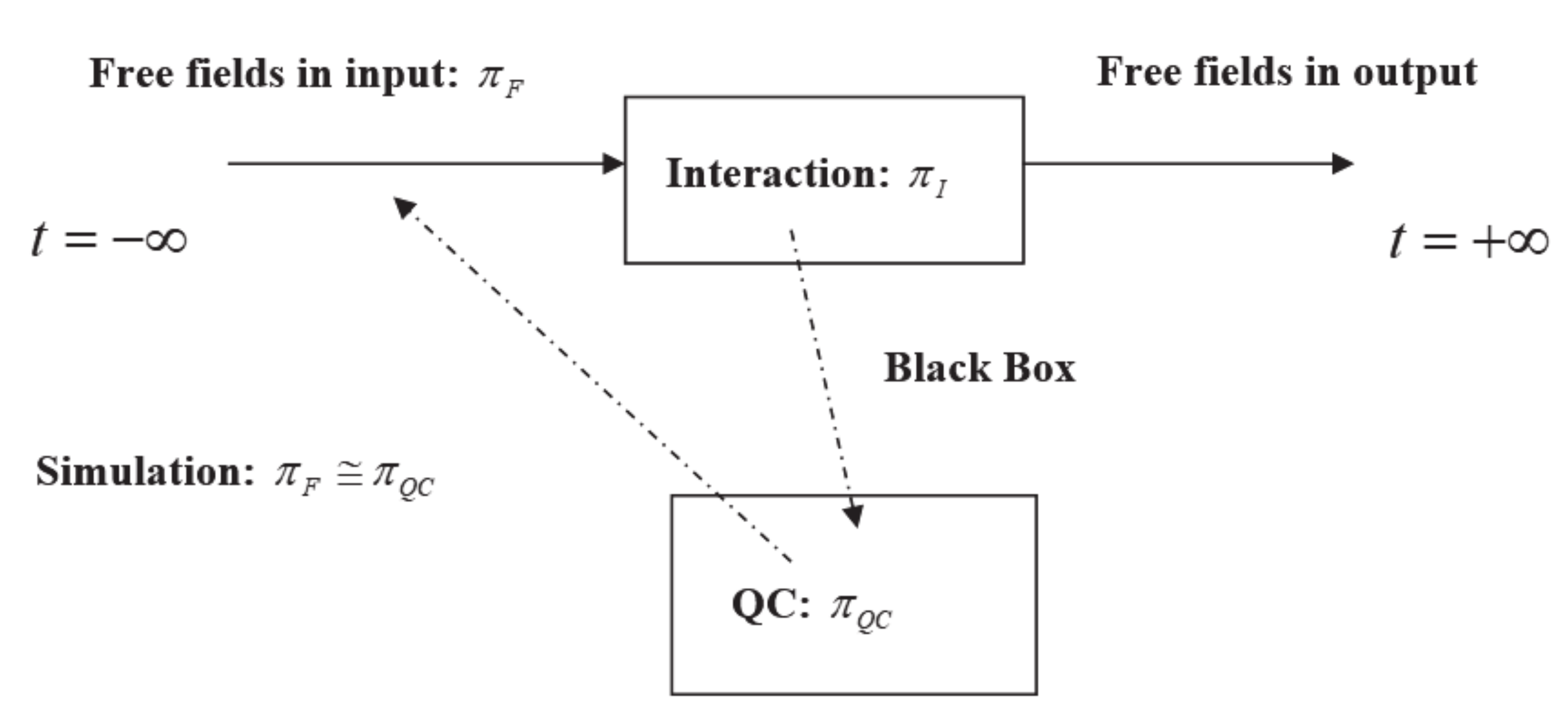
However, there is a conceptual, foundational problem in using quantum computers for simulating QFT, which arises from Haag’s theorem [4], which states that free and interacting fields must necessarily be defined on unitarily inequivalent Hilbert spaces. So suppose that a scattering process must be simulated by a quantum computer. This is impossible in principle, because the quantum computer is a quantum mechanical system, with a finite number of degrees of freedom, which, according to von Neumann’s theorem, has only unitarily equivalent representations. In other words, if the quantum computer simulates free input fields, let us say in representation ${\pi }_F$ (where the subscript F stands for “free”) it cannot also simulate their interaction in representation ${\pi }_I$ (where the subscript I stands for “interacting”) because it does not exist a unitary transformation $U:H_F\to H_I$ such that ${\pi }_F=U^{†}{\pi }_{I}U$. Then the interaction process will be a black box for the quantum computer. See Figure 8.

The ${\pi }_I$, ${\pi }_F$, ${\pi }_{QC}$ indicate the representations for the interacting fields, the free fields and the QC respectively. The ${\pi }_I$, ${\pi }_F$ are not unitarily equivalent to each other for Haag’s theorem. The ${\pi }_{QC}$ representations are all unitarily equivalent for the Stone-von Neumann theorem. Then, if ${\pi }_{QC}$ can be unitarily equivalent to ${\pi }_F$, cannot be also unitarily equivalent to ${\pi }_I$. Then, the interaction appears as a black box to the QC, and cannot be simulated.

Although the formulation of S-Matrix is such that one can find the final state by operating S-Matrix on the initial state without taking into account the moment of interaction, regarding it as a black box, the interaction cannot be simulated by a QC. In fact, it is the moment of interaction that all of the classes of representations may become equally important, and instead the QC is endowed with only one class.

Hence, the “for all useful purposes” black box of the S matrix formulation becomes a true black box with regards to quantum simulation.

So, in principle, we will not be able to directly simulate interacting quantum fields. However, quantum simulation might become possible once quantum fields are reduced to a quantum network of qubits. A seemingly argument was proposed by Preskill [13] and by Jordan et al. [14], who recognized that in order to build up an efficient quantum algorithm to quantum simulate the ${\phi }^4$ theory, the field should be “represented with finitely many qubits by discretization of space via a lattice, and discretization of the field value at each lattice site”.

In this work, we have shown that a (bosonic) QFT has in itself a hidden quantum information I_QFT. Extracting this quantum information, involves the reduction of QFT to a quantum-mechanical system, which is a quantum network, the Hidden Quantum Network (HQN) like the one shown in Figure 1.

Now, if we think of an external quantum simulator QC_E, with which we would like to simulate the QFT, we would simulate in fact the HQN, not the original QFT, because the QFT ceased to exist once it revealed the quantum information I_QFT it hid. However, in some sense, the quantum network HQN is a kind of “skeleton” of the original QFT, from which we could go back to QFT.

We state the following no-go theorem:

“If it exists a representation ${\pi }_{QC}$ of the quantum simulator which is unitarily equivalent to the representation ${\pi }_F$ of the free fields, then it does not exist a representation ${\pi }_{QC}\text{'}$ of the quantum simulator that is unitarily equivalent to the representation ${\pi }_I$ of the interacting fields.” This means, in practice, that a quantum algorithm for simulating QFT will be incomplete, unless quantum QFT is reduced to a quantum network HQN, which has only one class of unitarily equivalent representations.

Now, the question is: “How can an external quantum computer simulate two interacting quantum networks HQN¹ and HQN²?”. The answer is given by “gluing” the two quantum networks as shown in Figure 9. However, before going further, we want to clarify what is meant here by the “bonding” of the two networks. To do this, it is worth remembering the existence of the “gluing operation”, introduced in the quantum metalanguage [43] which controls the logic of quantum information.

Given the quantum sequent $\left|{-}^{{\lambda }_i}{p}_i\right.$ ($i\in N$) (a quantum assertion in the metalanguage) where ${\lambda }_i\in C$ is the assertion degree, and $p_i$ are atomic propositions of the quantum logic (the quantum object language), and its *-dual (also defined in [42]) $p_i\left|{-}^{{\lambda }_i}{}^{*}\right.$, where ${\lambda }_i{}^{*}$is the complex conjugate of ${\lambda }_i$, we make their gluing by means of the gluing operation “ “ defined as: $\left(p_i\left|{-}^{{\lambda }_i}{}^{*}\right.\right)$ $\left(\left|{-}^{{\lambda }_i}{p}_i\right.\right)=p_i\left|{-}^{\left|{\lambda }_i\right|}{}^{2}p{}_i\right.$, with the meta data ${\displaystyle \sum _i{\left|{\lambda }_i\right|}^2=1}$.

Note that the quantum identity axiom $p_i\left|{-}^{\left|{\lambda }_i\right|}{}^{2}p{}_i\right.$ bears a partial truth value $v_i={\left|{\lambda }_i\right|}^2$, which can be interpreted as the probability with which a quantum object can be identical to itself. Regarding the bonding of the two networks, we will interpret the quantum fields of the boson as statements (assertions) of a quantum metalanguage (work in progress). More precisely, we identify the incoming fields ${\left|{\varphi }_i\right.〉}_{IN}$ with the quantum assertion $\left|{-}^{{\lambda }_i}{p}_i\right.$, and the outgoing fields ${\left|{\varphi }_i\right.〉}_{OUT}\equiv {\left.〈{\varphi }_i\right|}_{IN}$ as the *-dual $p_i\left|{-}^{{\lambda }_i}{}^{*}\right.$.

Hence, the gluing of the two quantum sequents corresponds to the bonding of the networks of incoming and outgoing fields $\left.〈{\varphi }_i\right|\left|{\varphi }_i\right.〉={\left|{\lambda }_i\right|}^2$ through the interaction, which is revealed by ${\left|{\lambda }_i\right|}^2$. In fact, a displacement of the boson field ${\varphi }_i\to {\varphi }_i+\delta {\varphi }_i$ gives ${\varphi }_i{}^{*}{\varphi }_i={\left|\delta {\varphi }_i\right|}^2$, then we conclude ${\left|\delta {\varphi }_i\right|}^2={\left|{\lambda }_i\right|}^2$. This means that the bonding of the incoming and outgoing networks is made possible through the interaction phase, which is dominated by a dressed vacuum, with a boson condensate density given by ${\left|\delta \varphi {}_i\right|}^2$.

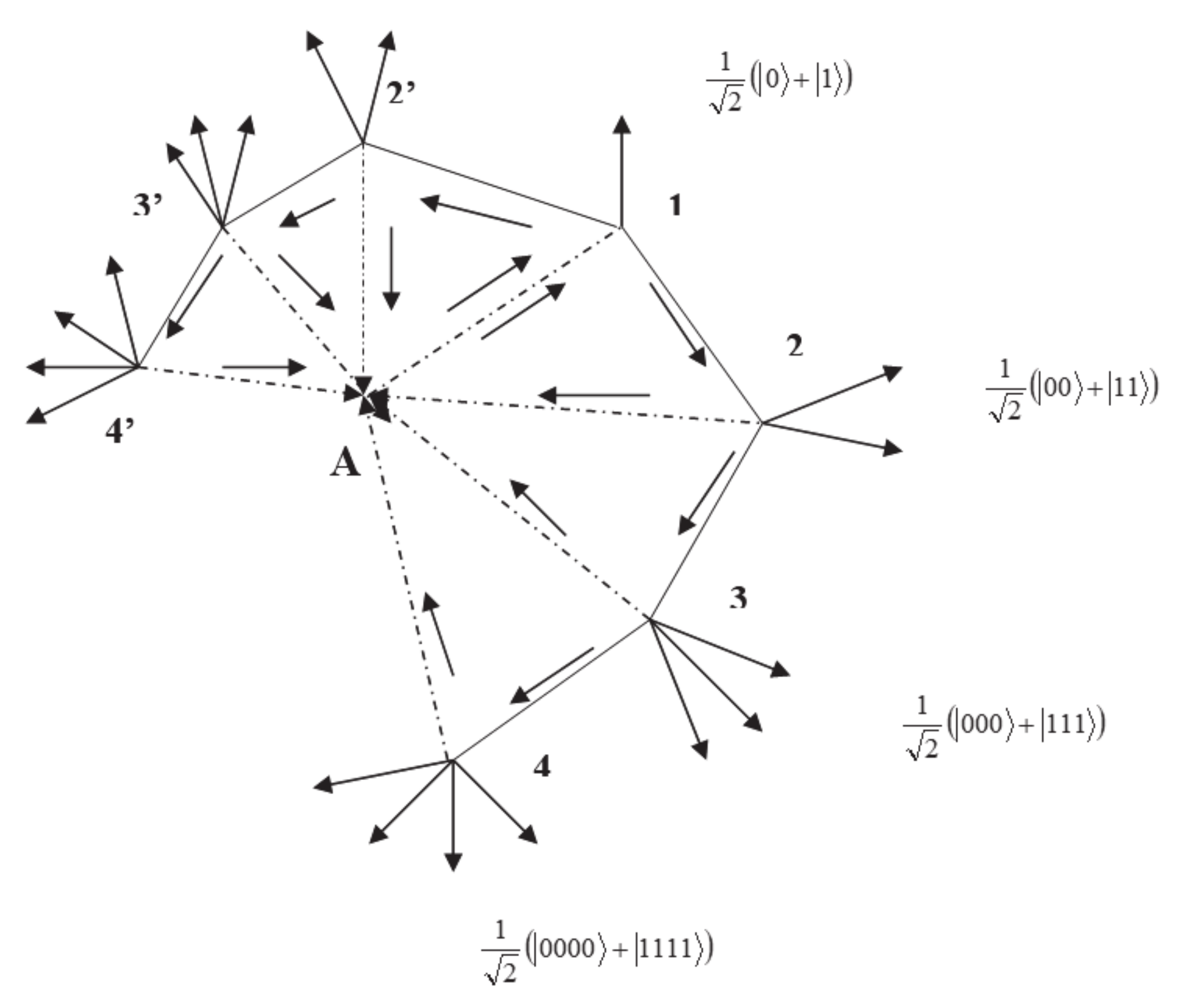
More details on this will be provided in a future article. Regardless, we just wish to add a little remark at this point. The probability with which a quantum object can be identical to itself, expressed by ${\left|{\lambda }_i\right|}^2$in the quantum identity axiom may be interpreted as the impossibility for the outgoing fields to be fully determined by the incoming ones, even in the case they are identical. The problem stands in the interaction, which is just made out of mixed states, designing informational ignorance.

The interaction net results from the bonding of two identical nets like that of Figure 1. The connected part of the graph describes the interacting fields. The disconnected part of the graph (the free outgoing arrows) describes the free fields: the input on the left, the output on the right. The primed and unprimed numbers that identify the nodes refer to the left and right networks respectively.

The connected part of the network in Figure 9 represents the interaction, and consists of fully mixed states (the dotted connecting links) and quantum fluctuations of the metric (the un dotted connecting links).

The connected part of the network is the most similar to a scale-free growing network, where free links are absent. However, the connected part is deterministic, in the sense that it follows some precise rules, as a lattice.

The disconnected part of the graph (outgoing free links), which consists exclusively of pure states that are maximally entangled, represents the free fields. The free links destroy the structure of a regular lattice, as the configuration of free links changes at each node.

Each node of the graph is associated with a quantum gate of the quantum simulator QC. The presence of maximally entangled states in the quantum network is crucial for quantum simulation, in fact entanglement was shown [44] to be necessary to achieve quantum computational speed-up.

By balancing the quantum entropy of the fully mixed states with the entanglement entropy of the maximally entangled states, it will be possible to simulate both the interacting fields and the free fields of the original QFT.

However, an important requirements is needed: The quantum simulator should be able to simulate mixed states. Actually, such a quantum computer has been described in [45], where the authors define a quantum circuit which is allowed to be in a mixed state and to use quantum operations as gates, not necessarily unitary.

It may be worth stressing the fact that the connected part of the graph in Figure 9 is filled of fully mixed states, whose maximum von Neumann entropy indicates our total ignorance of the interaction process in the original QFT.

Ignoring the connected part of the quantum network in Figure 9, is what one does in discarding the mathematical formalism of interactions in QFT, as often happens in constructivist formulations of QFT: only free fields in input and output are taken into account. If virtual states and mixed states were absent in the quantum network of Figure 9, the computational speed would be much lower. In fact, in this case, the quantum network would be reduced to a $2^n$ Boolean lattice (n = 0,1,2,....) represented by the regular tree graph (a binary tree) in Figure 10.

A (classical) abstract data structure (ADS), a binary tree, is what is left when the connected part of the interaction net of Figure 9 is removed.

The dramatic consequences of ignoring the quantum-computational structure of the interaction process will be discussed, among other topics, in Section 9.

9. The Quantum Black Hole Paradigm

Quantum information theory states that QFT probably does not have explicit quantum information content, unlike QM. However, the question of entanglement in QFT has already been studied in the literature, for example in [46,47].

In [46] the authors show the existence of entanglement between internal and external particles with respect to the event horizon of a black hole, and that this entanglement is a consequence of the existence of unitarily inequivalent representations of the CCR in QFT. In our opinion, their results have a common basis to ours, even if the contexts may appear different. In fact, as is well known, a black hole is the best scenario for studying quantum gravity, so entanglement in QFT, unitarily inequivalent representations of quantum fields and quantum gravity appear to be intimately interconnected. The same holds in the present paper, where however the difference lies in the fact that our quantum gravity scenario is that of Wheeler space-time quantum foam at the Planck scale.

In [47] (specifically in the Appendix) the authors showed in detail that in QFT an entangled state can be viewed as a collective mode vacuum $\left|0\left(\theta \right)\right.〉$controlled by the Bose–Einstein condensation. Such an entangled state is unitarily inequivalent to the bare vacuum $\left|0\right.〉$, which is non-entangled.

In other words, in QFT there is unitary inequivalence between the entangled and non-entangled state.

This fact is very important in our case, since it applies quite well to the quantum network in Figure 9. Indeed, the connected part of that network, which is not entangled, describes the interacting fields, while the disconnected, entangled part describes the free fields. In a sense, we could rephrase Haag’s theorem, which states that the representation of interacting fields is unitarily inequivalent to that of asymptotic free fields, as follows: “In QFT interacting fields are (fully) mixed and asymptotic free fields are (maximally) entangled, and there is no a unitary transformation between the two phases.”

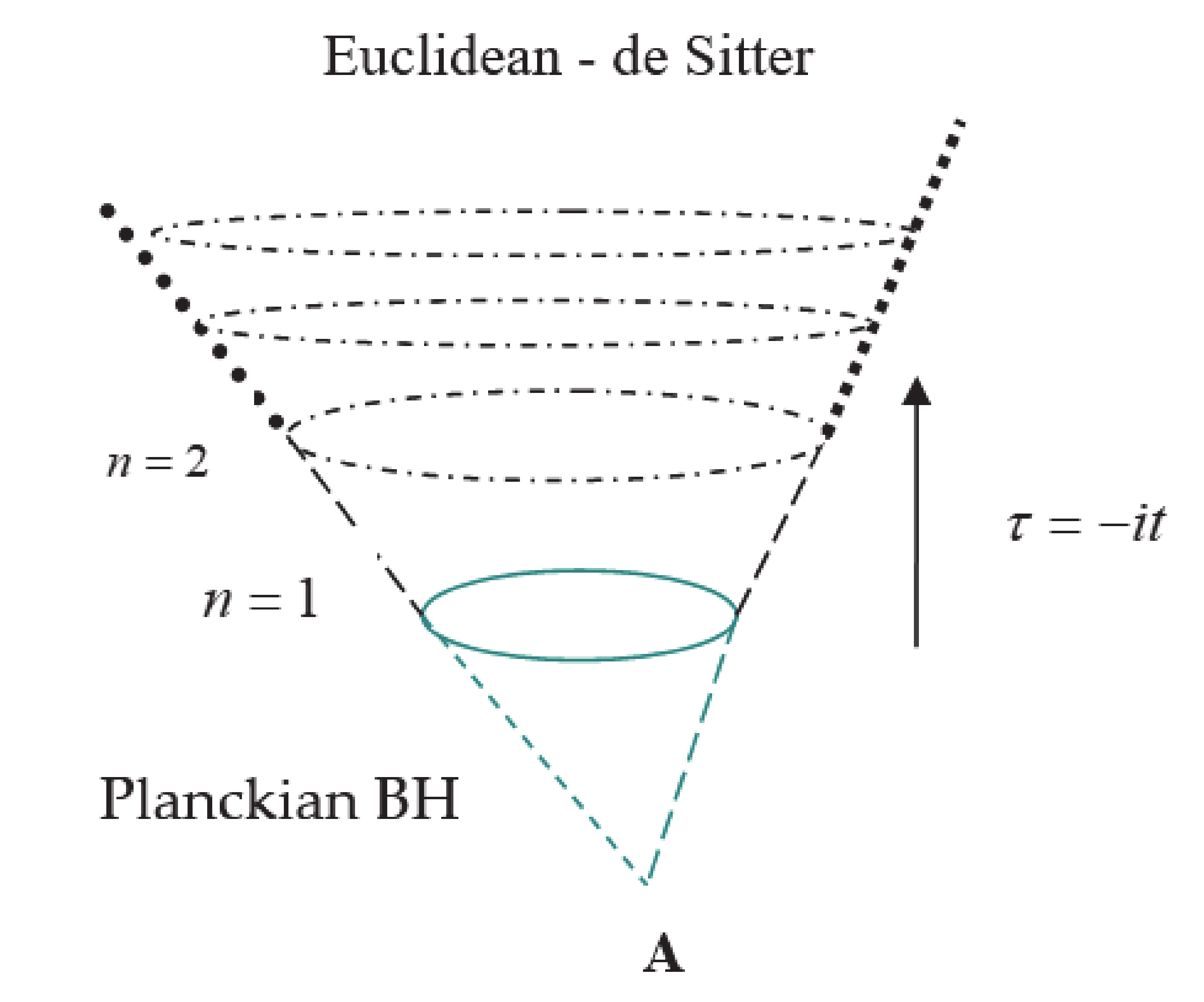
A (quantum) Euclidean de Sitter universe [32] on which the present work was based, can be seen as the expansion of a Euclidean Planckian BH, the latter being present at level $n=1$. It should be reminded that, while a BH has an absolute horizon, a de Sitter universe has an observer-dependent horizon. This means that an observer on the nth hypersurface at $t=t_n$will receive signals from all the other hypersurfaces at $t_{n\text{'}}$, with $n\text{'}<n$ but not from those with $n\text{'}>n$. Only at the Planck scale $\left(n=1\right)$ does the de Sitter horizon become an absolute horizon, as it coincides with the Schwarzschild radius of a Planckian black hole [32]. 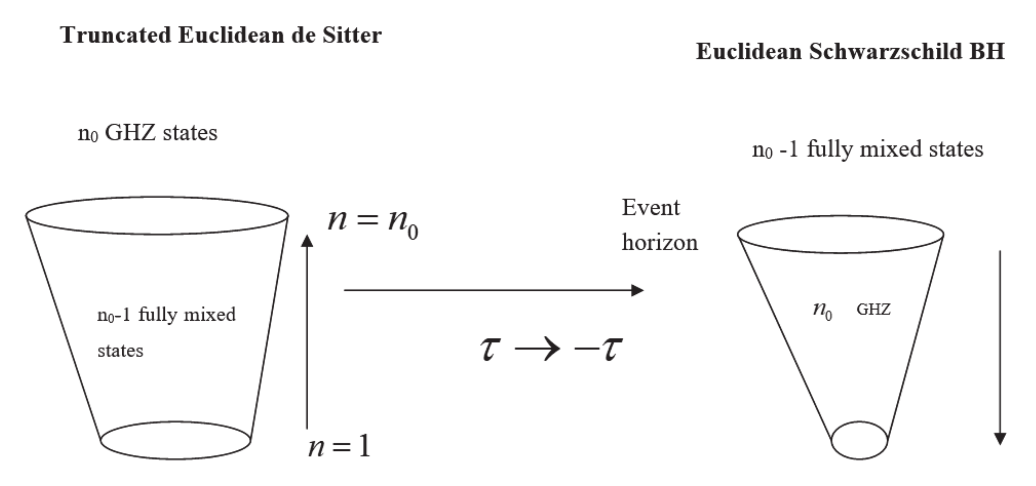See Figure 11. However, by truncation (at a given level $n=n_0$), and under the $\tau \to -\tau$ transformation (where $\tau =-it$ is the imaginary time) the Euclidean quantum de Sitter universe can be viewed as a Euclidean Schwarzschild BH [48,49] (see Figure 12). Then, at a given level $n_0$, the connected part of the network in Figure 9, which consists of fully mixed states, is the exterior of the quantum BH event horizon, while the disconnected part, which consists of pure (maximally entangled) states is the interior.

As Hawking [50] pointed out, the fact that a pure state cannot evolve into a mixed state by a unitary transformation implies that information is lost. However, as we have shown in this article, based on a quantum de Sitter space-time, quantum information is not lost in the mixed states of the interaction phase once all the pure states of the asymptotically free phase of the fields are maximally entangled. Applying this result to the inverse case of the black hole, in the extreme hypothesis that all pure states within a black hole are maximally entangled, the evaporation of the black hole would not cause a loss of information.

The non-existence of a unitary transformation that makes a pure state evolve into a mixed state can then be understood as the non-existence of a unitary transformation between the interacting fields representation and that of asymptotically free fields, according to Haag’s theorem.

The classical singularity “A” in Figure 9 might be seen as the black hole singularity where all degrees of freedom would be lost, however it is not so, because a Planckian BH and the de Sitter universe are Euclidean, so they are singularity free.

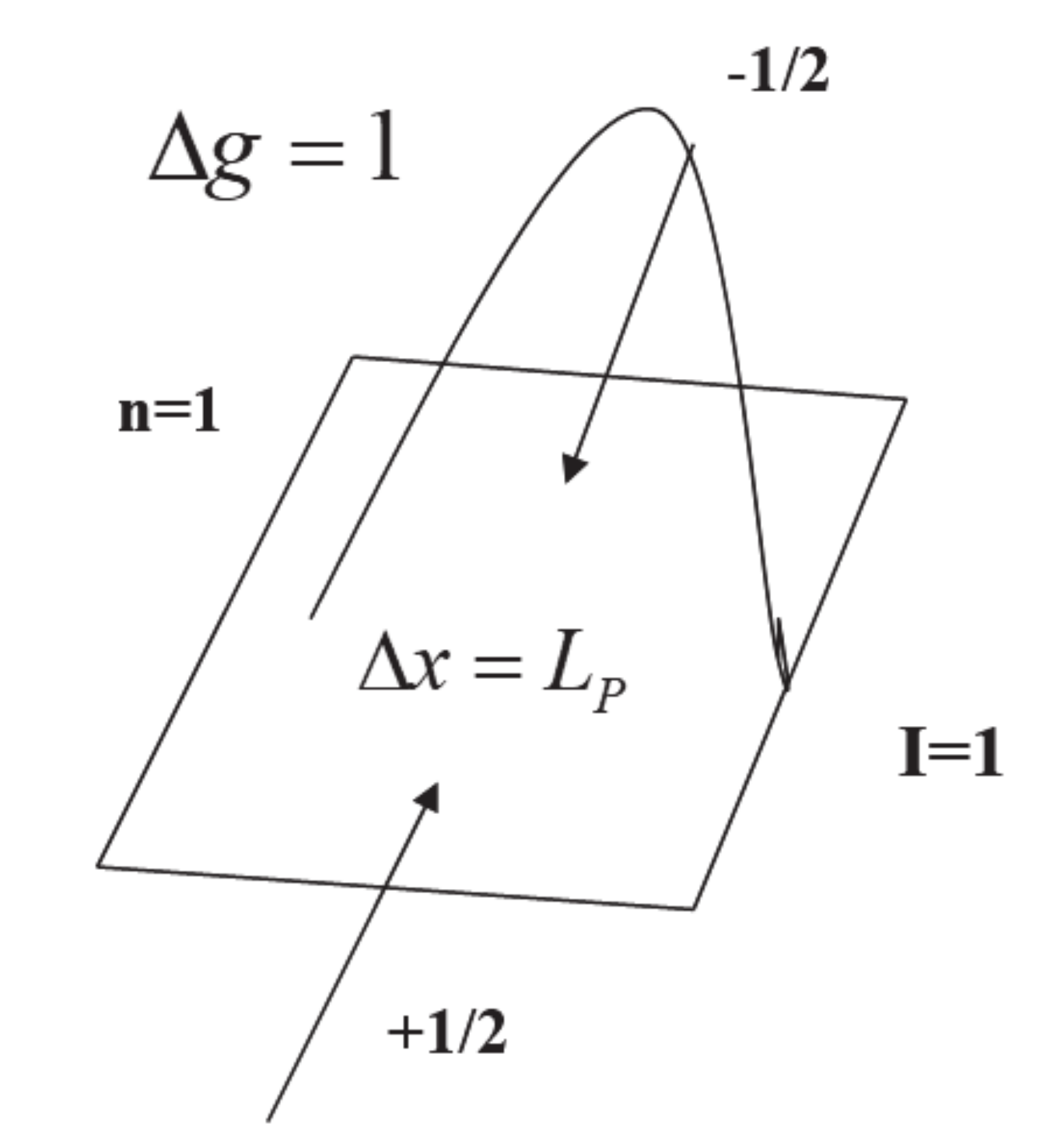
The Planckian black hole, which originates the quantum de Sitter universe can be also depicted (see Figure 13) as the “level” $\left(n=1\right)$ of the quantum network discussed in this paper. There, the uncertainty in the position state is equal to the Planck length $\left(\Delta x=L_P\right)$, the quantum fluctuation of the metric is maximal $\left(\Delta g=1\right)$, and the quantum information is minimal $\left(I=1\right)$ as the Planckian pixel encodes one qubit. In fact, a pixel can be “on” = 1 and “off“ = 0 at the same time, (i.e., it can be interpreted as a qubit) [37] if the puncture is made by a (open) spin nework’s edge [51] in the superposed quantum state: $\frac{1}{\sqrt{2}}\left(\left|\frac{1}{2}\right.〉\pm \left|-\frac{1}{2}\right.〉\right)$.

For $n=1$ (at the Planck scale), $\left(I=1\right)$, we have only one puncture giving rise to one pixel of area, associated with the 1-qubit state $\left|1\right.〉=$$\frac{1}{\sqrt{2}}\left(\left|on\right.〉\pm \left|off\right.〉\right)$, which represents the horizon state of a Euclidean Planckian black hole [32]. In summary, At level n = 1 of the quantum network, the uncertainty $\Delta x$ in the position state of the bosonic field, induced by the maximum fluctuation of the metric $\Delta g=1$, is equal to the Planck length. The surface of the sphere of radius has the area of a Planckian pixel, which is the area of the event horizon of a Planckian BH. The content of the information is one qubit, encoded by the pixel according to the quantum holographic principle [36]. So there is only one pure state within the event horizon and there are no mixed states outside. This is why a Planckian BH does not evaporate. It seems that the uncertainty in the position state of the boson field creates a Planckian BH, from which a Euclidean quantum de Sitter universe originates.

Level $n=1$ of the quantum network corresponds to the (absolute) event horizon of a Planckian BH (the undotted blu circle) from which a Euclidean de Sitter universe originates (see the arrow), which has an observer-dependent horizon at each level n (the dotted circles).

The attractor A of the quantum network is not a true singularity.

A Euclidean quantum de Sitter universe truncated to a fixed level $n=n_0$ corresponds, by$\tau$-inversion, to a Euclidean Schwarzschild BH. The n₀ − 1 completely mixed states within the horizon of the truncated Euclidean universe become the mixed states outside the BH event horizon, and the n₀ maximally entangled states on the n₀th de Sitter horizon become the pure states within the BH event horizon.

The curved line represents the quantum fluctuation of the metric, which, at level n = 1 is maximal ($\Delta g=1$). The square stands for the planckian pixel. Inside the square, $\Delta x$ stands for the uncertainty in the position state, and $L_P$ is the Planck length. The two arrows denote the puncture made by a spin ½ edge in a superposed quantum state. I = 1 is the quantum information of one qubit.

10. Discussion and Conclusions

In this paper we have illustrated a particular process of reduction from QFT to QM. This reduction mechanism proved to be much more complex than just the reduction to finite volume. In fact, some unknown characteristics emerged and several topics were involved.

Among the unknown characteristics there is the quantum-computational structure which is intrinsically rooted in QFT, and the quantum-gravitational origin of this same structure. Among the topics involved, besides those of quantum information and quantum gravity, there are non-commutative geometry (the fuzzy sphere) and quantum simulation. The latter is of great importance as a possible theoretical support for practical applications in scattering processes of elementary particles at high energies. Until now, quantum algorithms to simulate QFT [13,14] have mainly used lattices.

A lattice is a particular type of regulator, which allows a computer simulation of QFT.

However, while a lattice breaks Lorentz’s invariance, our regulator does not, because a fuzzy sphere has the same rotational symmetry as the ordinary sphere. As Maas writes in his lectures [52]: “... it is an unfortunate consequence of our current understanding of quantum field theory that the need to have regulators always implies that some symmetries are broken, no matter what, until the regulator it is not removed”. It should be noted, however, that Lorentz’s invariance is restored on the fuzzy sphere.

A lattice is a mathematical artefact, as also Preskill says in [13]: “The lattice is an artifice introduced for convenience.” In our case, instead, the regulator is physical, because the discretization is induced by the quantum fluctuations of the metric in the attractor basin.

Also, while in the case of a reticular regulator the limit of the continuum is reached (but not always) when the number of sites is huge and the spacing approaches zero, in our case there is the classic limit that is reached when the fluctuations of the quantum metrics vanish near the attractor.

Moreover, while in the case of a reticular regulator the reduction of QFT to QM is not mathematically explicit, in our case it is, since the ansatz corresponds to the execution of a boson translation (as it was illustrated in Section 4). This shows how the unitarily inequivalent representations of QFT are reduced to a single class of unitarily equivalent representations of QM.

In Preskill’s algorithm for simulating scalar field theories, it was introduced a spatial lattice. To make the theory simulated, they replace the scalar field $\mathsf{\Phi }\left(\stackrel{\rightharpoonup }{x}\right)$ at each lattice site by a discrete variable with a finite number N of mutually orthogonal eigenstates. There is a conjugate variable $\pi \left(\stackrel{\rightharpoonup }{x}\right)$, the field momentum at the lattice site $\stackrel{\rightharpoonup }{x}$, which is related to $\mathsf{\Phi }\left(\stackrel{\rightharpoonup }{x}\right)$ by the quantum Fourier transform applied to the N-dimensional Hilbert space residing at each lattice site $\stackrel{\rightharpoonup }{x}$. For $N=2^n$, the quantum state of the field at a site can be encoded in n qubits.

In our case instead, qubits are induced directly by the quantum fluctuations of the metric, due to the uncertainty relationship between metric and quantum information.

Both approaches can lead to satisfactory results, but ours is more physical, not only in a heuristic sense, since it is supported by a rigorous mathematical framework. As Preskill himself says in [13]: “There may be more clever ways of regulating that would improve the efficiency of the simulation”.

In any case, however, the profound philosophical meaning of the mathematical role of a regulator is that by reducing the infinite degrees of freedom of QFT to a finite number, allows the quantum simulator and the simulated quantum system to have unitarily equivalent representations even when interactions are present.

Then, it may not be quite true that a quantum computer can simulate any quantum system, and our doubt is shared by Preskill in [13]. We claim that a quantum computer can simulate the hidden quantum network (HQN) of the quantum system under study. More precisely, a quantum computer can be programmed to be in a one-to-one correspondence with the HQN.

We think that QFT is meta-logically described (work in progress) by a “quantum metalanguage” (QML). If that is true, then QFT is its own semantics (QFT interprets itself). In the reduction process illustrated in this paper, QFT would appear then as the semantics of the quantum logic underlying the quantum information hidden in it. The reduction process (in particular the regulator) would then play the role of a definitional equation [53], which allows the switch from a metalanguage to an object language (the logic). In particular, the quantum version [43] of the definitional equation allows to pass from a QML to the quantum logic of quantum information (QLI).

Hence, the metalinguistic links between assertions, which are interpretable as interactions of quantum fields, are sent to logical connectives between propositions, which correspond to quantum correlations such as quantum superposition and entanglement.

Then, the definitional equation corresponds to the regulator of QFT discussed in this paper. In this logical framework, Haag’s theorem simply translates the fact that the QML contains the QLI, as every metalanguage contains the object language. Another important point to discuss is that of the serious consequences of the attitude of discarding the ontology of processes (in this case the ontology of interaction). As we have already pointed out in Section 8, the quantum network in Figure 9 consists of a connected part (which describes the interaction) and a disconnected part (which describes the free fields). So, ignoring the interaction process is tantamount to eliminating the connected part of the quantum network in Figure 9. The problem, unfortunately, is not only mathematical, but also physical. In fact, by eliminating the connected part of the graph, the balance between the quantum entropy of fully mixed states and the entanglement entropy of the maximum entangled states is lost. This involves the non-conservation of quantum information.

In fact, the result of neglecting the connected part of the quantum graph in Figure 9 reduces the latter to a pair of binary trees like the one in Figure 10, one for the input fields and the other for the output fields.

In this way, a Boolean lattice, a binary tree, which is an abstract data type used in computer science, would appear to be the classical computational skeleton of the original QFT, which makes no sense. In fact, as we said before, the computational skeleton of a quantum field theory is quantum. Using a binary tree to trace the original QFT would mean not recovering the quantum characteristics of the latter.

A fairly unexpected result of this article is that quantum gravity seems to be hidden in QFT just like quantum information does (remember that there is an uncertainty relationship between metric and quantum information). Indeed, the quantum fluctuations of the metric appear in this model within the attractive basin and induce uncertainty in the position states, leading to the definition of qubit states.

The structure of quantum foam arising in the attractor basin was exploited in Section 9 to show that the quantum network of information hidden in QFT seems to be closely related to the information loss paradox in evaporation of black holes, which then might be solved in the extreme hypothesis that all the pure states within the BH event horizon are maximally entangled.

It would be worth further looking for a series of relationships between QFT, QM, quantum information, entangled space-time, quantum gravity, non-commutative geometry, quantum metalanguage and quantum logic, since these topics are closely intertwined.

QM and QFT are not at the same level, neither mathematical (due to the appearance of the uir of the CCR in QFT, while in QM this is prohibited by Stone-von Neumann’s theorem) nor logical (QFT is described by a quantum metalanguage while QM is described by a quantum logic), neither physical (since Haag’s theorem holds in QFT, and therefore the irreducible representations of free fields are unitarily inequivalent to those of interacting fields).

Moreover, QM has a classical space-time background, which is absolute. Instead, we believe that QFT should have an entangled quantum space-time [54] as a space-time background. If you remove the QFT from the background, what remains is the entangled space-time, which is itself a quantum network, quite similar to that depicted in Figure 1. Some relations between the entangled space-time background and meta-logic may be found in a recent paper [55].

To conclude, in this work we have shown that a (bosonic) quantum field theory T has in itself a hidden quantum information I_T. Extracting this quantum information, however, involves the reduction of T to a quantum-mechanical system, which is a quantum network Q_T like the one shown in Figure 1.

Now if we think of an external quantum simulator Q_E, with which we would like to simulate T, we would actually simulate at least Q_T, not T, because the latter ceased to exist once it revealed the quantum information I_T it hid. In a sense, however, Q_T is T’s “skeleton”, and from it we can go back to T, at least that’s hope. It might be worth extending this reduction mechanism to fermionic QFT.