Selective Engineering for Preparing Entangled Steady States in Cavity QED Setup


Abstract
1. Introduction
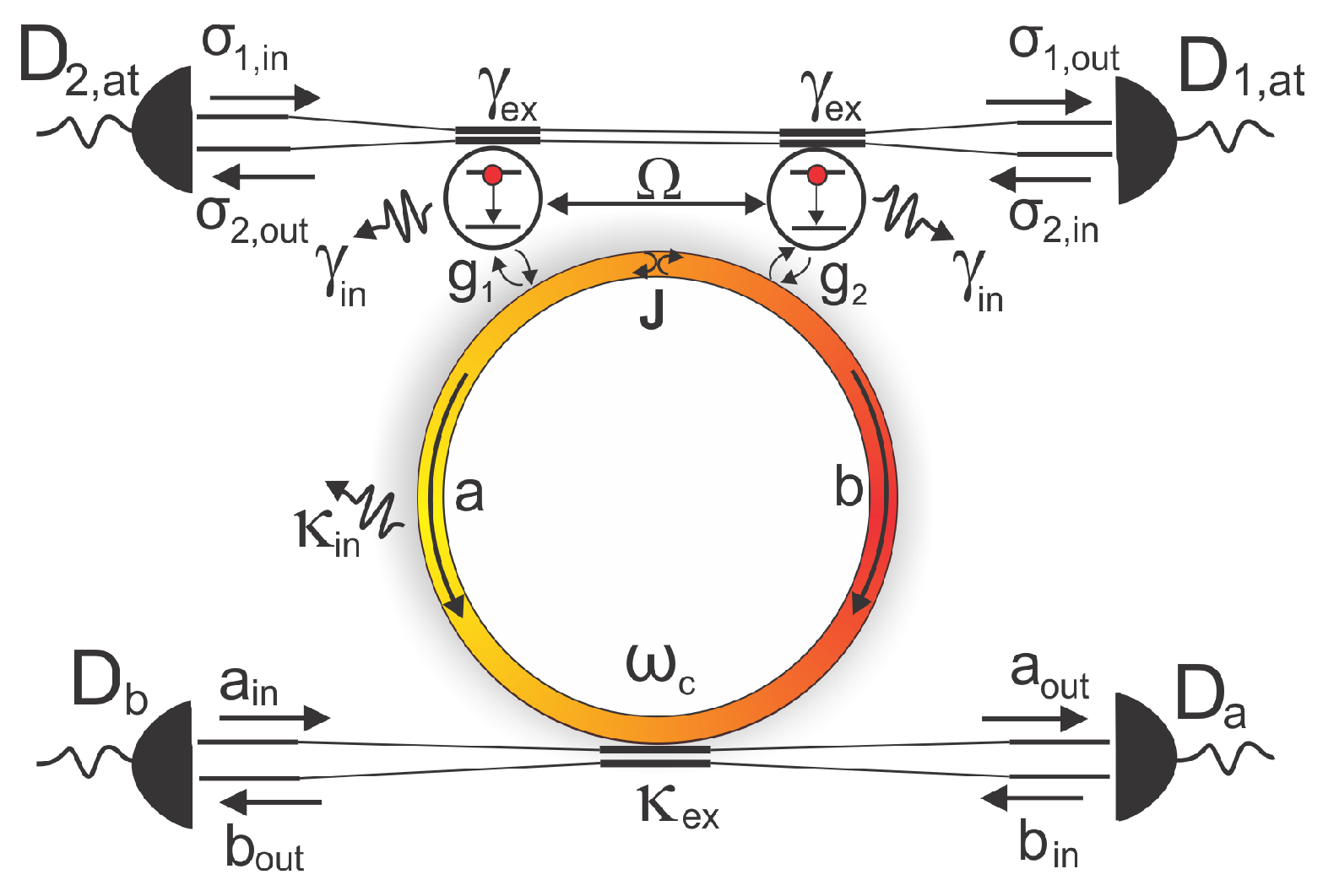
2. Model
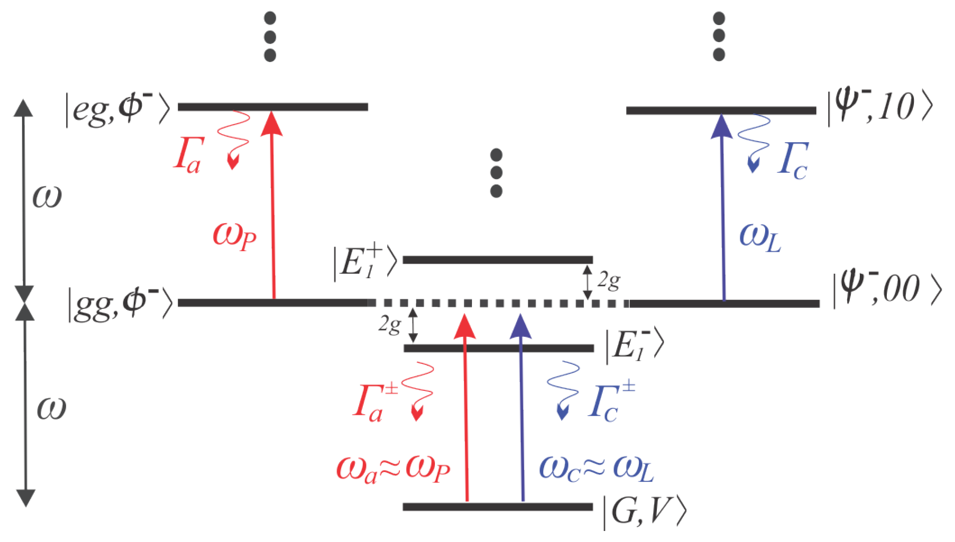
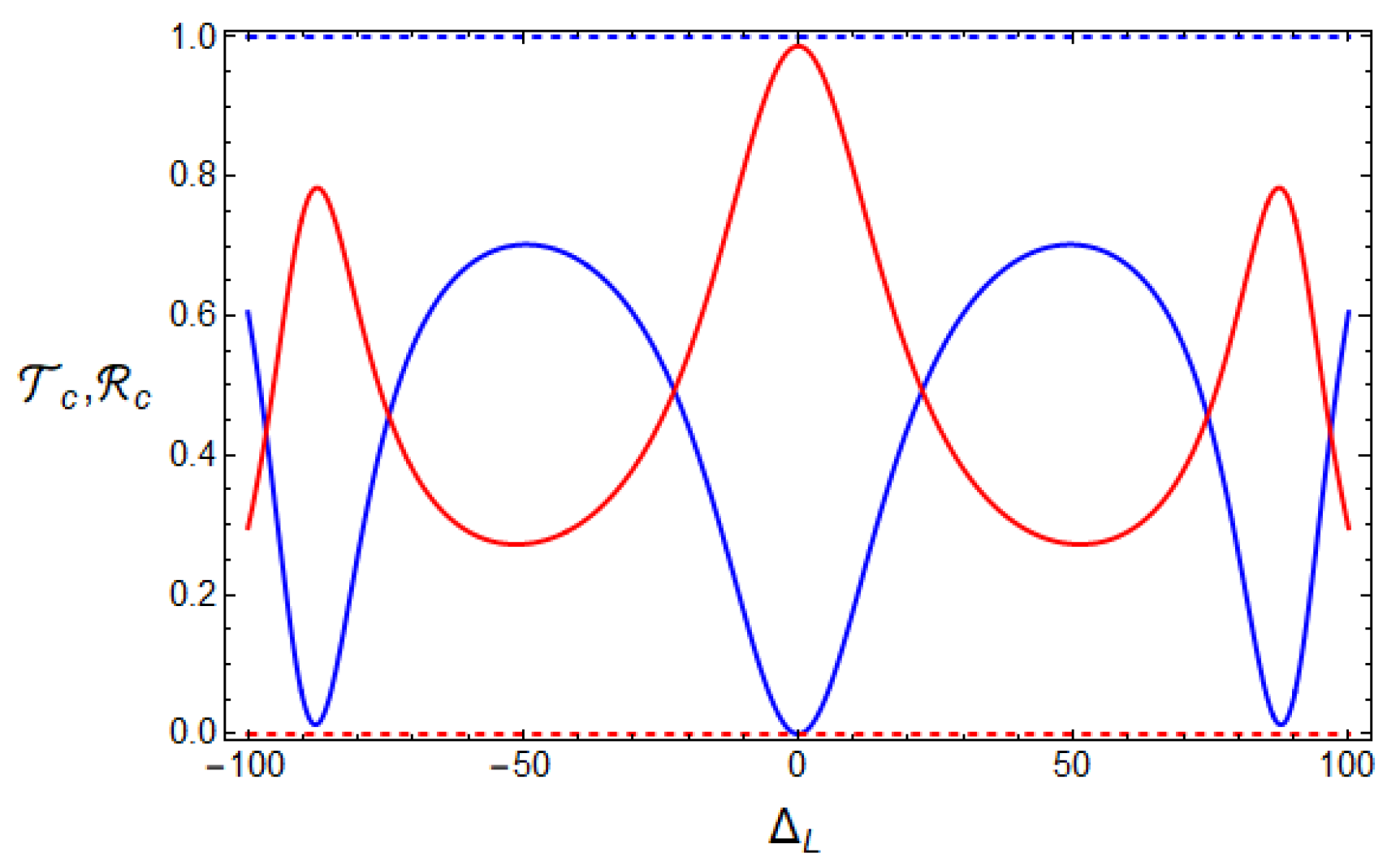
3. Monitoring the Atom–Cavity System by Driven the Cavity Mode
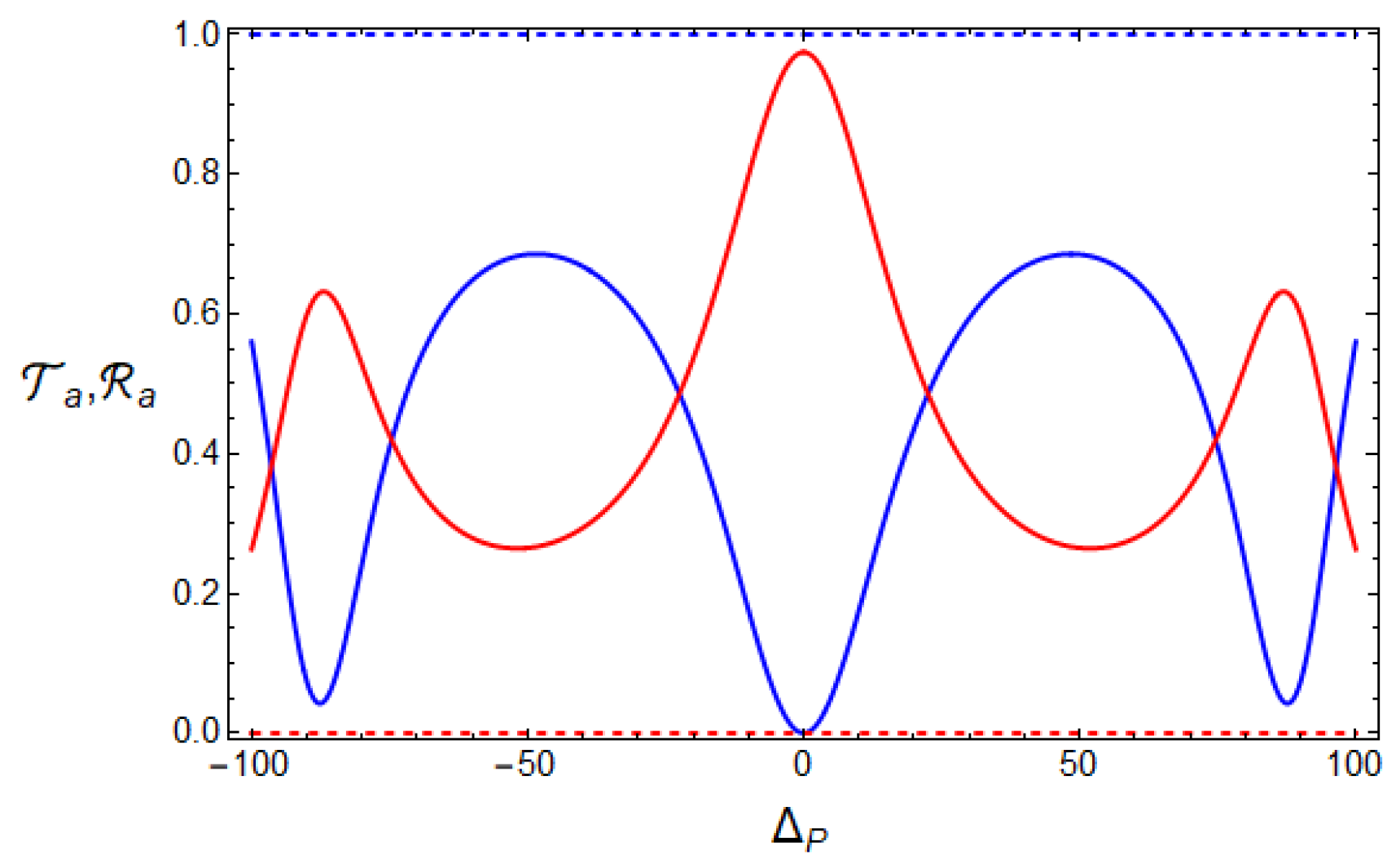
4. Monitoring the Atom–Cavity System by Driven the Single Atom
5. Transfer of Entanglement between Two Atoms and Two Modes
6. Conclusions
Author Contributions
Funding
Acknowledgments
Conflicts of Interest
References
- Horn, K.P.; Reiter, F.; Lin, Y.; Leibfried, D.; Koch, C.P. Quantum optimal control of the dissipative production of a maximally entangled state. New J. Phys. 2018, 20, 123010. [Google Scholar] [CrossRef]
- Jin, Z.; Su, S.L.; Zhu, A.D.; Wang, H.F.; Zhang, S. Dissipative preparation of distributed steady entanglement: An approach of unilateral qubit driving. Opt. Express 2017, 25, 88–101. [Google Scholar] [CrossRef] [PubMed]
- Kastoryano, M.J.; Reiter, F.; Sørensen, A.S. Dissipative Preparation of Entanglement in Optical Cavities. Phys. Rev. Lett. 2011, 106, 090502. [Google Scholar] [CrossRef] [PubMed]
- Stannigel, K.; Rabl, P.; Zoller, P. Driven-dissipative preparation of entangled states in cascaded quantum-optical networks. New J. Phys. 2012, 14, 063014. [Google Scholar] [CrossRef]
- Ma, S.L.; Li, Z.; Fang, A.P.; Li, P.B.; Gao, S.Y.; Li, F.L. Controllable generation of two-mode-entangled states in two-resonator circuit QED with a single gap-tunable superconducting qubit. Phys. Rev. A 2014, 90, 062342. [Google Scholar] [CrossRef]
- Arenz, C.; Cormick, C.; Vitali, D.; Morigi, G. Generation of two-mode entangled states by quantum reservoir engineering. J. Phys. B Atomic Mol. Opt. Phys. 2013, 46, 224001. [Google Scholar] [CrossRef][Green Version]
- Petiziol, F.; Dive, B.; Carretta, S.; Mannella, R.; Mintert, F.; Wimberger, S. Accelerating adiabatic protocols for entangling two qubits in circuit QED. Phys. Rev. A 2019, 99, 042315. [Google Scholar] [CrossRef]
- Mirza, I.M.; Schotland, J.C. Two-photon entanglement in multiqubit bidirectional-waveguide QED. Phys. Rev. A 2016, 94, 012309. [Google Scholar] [CrossRef]
- Macrì, V.; Nori, F.; Kockum, A.F. Simple preparation of Bell and Greenberger-Horne-Zeilinger states using ultrastrong-coupling circuit QED. Phys. Rev. A 2018, 98, 062327. [Google Scholar] [CrossRef]
- Mirza, I.M.; Schotland, J.C. Multiqubit entanglement in bidirectional-chiral-waveguide QED. Phys. Rev. A 2016, 94, 012302. [Google Scholar] [CrossRef]
- Mirza, I.M. Controlling tripartite entanglement among optical cavities by reservoir engineering. J. Mod. Opt. 2015, 62, 1048–1060. [Google Scholar] [CrossRef][Green Version]
- Mirza, I.M. Bi- and uni-photon entanglement in two-way cascaded fiber-coupled atom–cavity systems. Phys. Lett. A 2015, 379, 1643–1648. [Google Scholar] [CrossRef]
- Cramer, M.; Plenio, M.B.; Flammia, S.T.; Somma, R.; Gross, D.; Bartlett, S.D.; Landon-Cardinal, O.; Poulin, D.; Liu, Y.K. Efficient quantum state tomography. Nat. Commun. 2010, 1, 149. [Google Scholar] [CrossRef] [PubMed]
- Grangier, P.; Levenson, J.A.; Poizat, J.P. Quantum non-demolition measurements in optics. Nature 1998, 396, 537. [Google Scholar] [CrossRef]
- Takashima, K.; Nishida, M.; Matsuo, S.; Hatakenaka, N. Quantum Nondemolition Measurement of a Superconducting Flux Qubit. AIP Conf. Proc. 2006, 850, 945–946. [Google Scholar] [CrossRef]
- Di Lisi, A.; Mølmer, K. Entanglement of two atomic samples by quantum-nondemolition measurements. Phys. Rev. A 2002, 66, 052303. [Google Scholar] [CrossRef]
- Lecocq, F.; Clark, J.B.; Simmonds, R.W.; Aumentado, J.; Teufel, J.D. Quantum Nondemolition Measurement of a Nonclassical State of a Massive Object. Phys. Rev. X 2015, 5, 041037. [Google Scholar] [CrossRef] [PubMed]
- Rossatto, D.Z.; Villas-Boas, C.J. Method for preparing two-atom entangled states in circuit QED and probing it via quantum nondemolition measurements. Phys. Rev. A 2013, 88, 042324. [Google Scholar] [CrossRef]
- Li, P.B.; Gao, S.Y.; Li, F.L. Quantum-information transfer with nitrogen-vacancy centers coupled to a whispering-gallery microresonator. Phys. Rev. A 2011, 83, 054306. [Google Scholar] [CrossRef]
- Jin, J.S.; Yu, C.S.; Pei, P.; Song, H.S. Positive effect of scattering strength of a microtoroidal cavity on atomic entanglement evolution. Phys. Rev. A 2010, 81, 042309. [Google Scholar] [CrossRef]
- Dayan, B.; Parkins, A.; Aoki, T.; Ostby, E.; Vahala, K.; Kimble, H. A photon turnstile dynamically regulated by one atom. Science 2008, 319, 1062–1065. [Google Scholar] [CrossRef] [PubMed]
- Aoki, T.; Parkins, A.S.; Alton, D.J.; Regal, C.A.; Dayan, B.; Ostby, E.; Vahala, K.J.; Kimble, H.J. Efficient Routing of Single Photons by One Atom and a Microtoroidal Cavity. Phys. Rev. Lett. 2009, 102, 083601. [Google Scholar] [CrossRef] [PubMed]
- Cohen-Tannoudji, C.; Dupont-Roc, J.; Grynberg, G. Atom-Photon Interactions: Basic Processes and Applications; Wiley-VCH: Weinheim, Germany, 1998; p. 678. ISBN 0-471-29336-9. [Google Scholar]
- Bullough, R.K. Photon, quantum and collective, effects from rydberg atoms in cavities. Hyperfine Interact. 1987, 37, 71–108. [Google Scholar] [CrossRef]
- Gardiner, C.W.; Collett, M.J. Input and output in damped quantum systems: Quantum stochastic differential equations and the master equation. Phys. Rev. A 1985, 31, 3761–3774. [Google Scholar] [CrossRef]
- Aghamalyan, D.; You, J.B.; Chu, H.S.; Png, C.E.; Krivitsky, L.; Kwek, L.C. Quantum transistor realized with a single Λ-level atom coupled to the microtoroidal cavity. arXiv 2019, arXiv:1902.11052. [Google Scholar]
- Vidal, G.; Werner, R.F. Computable measure of entanglement. Phys. Rev. A 2002, 65, 032314. [Google Scholar] [CrossRef]


© 2019 by the authors. Licensee MDPI, Basel, Switzerland. This article is an open access article distributed under the terms and conditions of the Creative Commons Attribution (CC BY) license (http://creativecommons.org/licenses/by/4.0/).
Share and Cite
Sousa, E.H.S.; Roversi, J.A. Selective Engineering for Preparing Entangled Steady States in Cavity QED Setup. Quantum Rep. 2019, 1, 63-70. https://doi.org/10.3390/quantum1010007
Sousa EHS, Roversi JA. Selective Engineering for Preparing Entangled Steady States in Cavity QED Setup. Quantum Reports. 2019; 1(1):63-70. https://doi.org/10.3390/quantum1010007
Chicago/Turabian StyleSousa, Emilio H. S., and J. A. Roversi. 2019. "Selective Engineering for Preparing Entangled Steady States in Cavity QED Setup" Quantum Reports 1, no. 1: 63-70. https://doi.org/10.3390/quantum1010007
APA StyleSousa, E. H. S., & Roversi, J. A. (2019). Selective Engineering for Preparing Entangled Steady States in Cavity QED Setup. Quantum Reports, 1(1), 63-70. https://doi.org/10.3390/quantum1010007