Article

Experimentally Accessible Witnesses of Many-Body Localization

1
Dahlem Center for Complex Quantum Systems, Freie Universität Berlin, 14195 Berlin, Germany
2
Department of Mathematical Sciences, University of Copenhagen, DK-2100 København, Denmark
3
Northrop Grumman Corporation, Baltimore, MD 21240, USA
*
Author to whom correspondence should be addressed.
Quantum Rep. 2019, 1(1), 50-62; https://doi.org/10.3390/quantum1010006
Submission received: 28 May 2019 / Revised: 12 June 2019 / Accepted: 13 June 2019 / Published: 17 June 2019

Abstract

:
The phenomenon of many-body localized (MBL) systems has attracted significant interest in recent years, for its intriguing implications from a perspective of both condensed-matter and statistical physics: they are insulators even at non-zero temperature and fail to thermalize, violating expectations from quantum statistical mechanics. What is more, recent seminal experimental developments with ultra-cold atoms in optical lattices constituting analog quantum simulators have pushed many-body localized systems into the realm of physical systems that can be measured with high accuracy. In this work, we introduce experimentally accessible witnesses that directly probe distinct features of MBL, distinguishing it from its Anderson counterpart. We insist on building our toolbox from techniques available in the laboratory, including on-site addressing, super-lattices, and time-of-flight measurements, identifying witnesses based on fluctuations, density–density correlators, densities, and entanglement. We build upon the theory of out of equilibrium quantum systems, in conjunction with tensor network and exact simulations, showing the effectiveness of the tools for realistic models.

1. Introduction

Many-body localization provides a puzzling and exciting paradigm within quantum many-body physics and is for good reasons attracting significant attention in recent years. Influential theoretical work [1] building upon the seminal insights by Anderson on disordered models [2] suggests that localization would survive the presence of interactions. Such many-body localized models, as they are dubbed, would be insulators even at non-zero temperature and exhibit no particle transport. Maybe more strikingly from the perspective of statistical physics, these many-body localized models would fail to thermalize following out of equilibrium dynamics [3,4,5], challenging common expectations how systems “form their own heat bath” and hence tend to be locally well described by the familiar canonical Gibbs ensemble [6,7,8]. Following these fundamental observations, a “gold rush” of theoretical work followed, identifying a plethora of phenomenology of such many-body localized models. They would exhibit a distinct and peculiar logarithmic scaling of entanglement in time [9,10], the total correlations of time averages have a distinct scaling [11], many Hamiltonian eigenstates fulfill area laws [12] for the entanglement entropy [13,14] and hence violate what is called the eigenstate thermalization hypothesis [15]. The precise connection and interrelation between these various aspects of many-body localization is just beginning to be understood [14,16,17,18,19,20], giving rise to a vivid discussion in theoretical physics.
These theoretical studies have recently been complemented by seminal experimental activity, allowing to probe models that are expected to be many-body localized in the laboratory under remarkably controlled conditions [21,22]. This work goes much beyond earlier demonstrations of Anderson localization in a number of models [23], in that now actual interactions are expected to be relevant. Such ultra-cold atomic systems indeed provide a pivotal arena to probe the physics that is at stake here [24]. What is still missing, however, is a direct detection of the rich phenomenology of many-body localization in the laboratory. Rather than seeing localization and taking the presence of interactions for granted, it seems highly desirable to make use of these novel exciting possibilities to directly see the above features, distinctly separating the observations from those expected from non-interacting Anderson insulators. Such a mindset is that of “witnessing” a property, somewhat inspired by how properties such as entanglement are witnessed [25,26,27] in quantum information.
In this work, we aim at capturing precisely those aspects of the rich phenomenology of many-body localization that are directly accessible with present experimental tools. We would like to provide a “dictionary” of possible tools, as a list or a classification of features that can be probed making use of only in situ site resolved measurements, including the measurement of density–density correlations and time of flight measurements, in conjunction with a variation of densities. In this way, we aim at identifying a comprehensive list of features that “could be held responsible” for MBL, based on data alone. While all we explicitly state is directly related to cold atoms in optical lattices, a similar approach is expected to be feasible in continuous cold bosonic atoms on atom chips [28,29], where correlation functions of all orders can readily be directly measured. We leave this as an exciting perspective.

2. Probing Disordered Optical Lattice Systems

The setting we focus on is that of interacting (spin-less) fermions placed into a one-dimensional optical lattice, a setting that prominently allows to probe the physics under consideration [21,24]. Such systems are well described by
H = j f j f j + 1 + h . c . + j w j n j + U j n j n j + 1 ,
where f j denotes a fermionic annihilation operator on site j and n j = f j f j is the local particle number operator. The disorder in the model is carried by the local potential-strength w j , which is drawn independently at each lattice site j according to a suitable probability distribution. Experimentally, the disorder can either be realized by superposing the lattice with an incommensurate laser or by speckle patterns [21]. From Equation (1), one obtains the disordered Heisenberg chain [30] by setting U = 2 and scaling the disorder by a factor two. To keep the discussion conceptually clear, as in Ref. [30], we make use of a uniform distribution on the interval [ I , I ] , where we refer to I as the disorder strength. Thus, for U = 2 the ergodic to MBL phase transition is approximately at I 7 [30]. Most of the known experiments of MBL have been carried out in a related model of on-site interacting bosons for which we show data in Appendix B.
The phase diagram of these models is best known for U = 0 corresponding to the non-interacting Anderson insulator and for U = 2 , the MBL phase. To add a flavor of usual phase transitions order parameters such as total correlations [11], fluctuations of local observables [31] or the structure of the eigenstates [32] have been suggested. While these quantities impressively signal the transition, it is not a priori clear whether they can be implemented in an actual experiment. Recent numerical studies [33] show that pump–probe type setups and novel instances of spin noise spectroscopy [34] as well as utilizing MBL systems as a bath [35] are indeed suited to distinguish the above phases, albeit experimental realizations of this endeavor appear to need substantial changes and innovations in realistic setups. Another possibility for the phase distinction, which has prominently been carried out experimentally [22], is given by observing the behavior of quasi two-dimensional systems in comparison to their one dimensional counterparts. While this impressively demonstrates the capabilities of optical lattices as platforms for quantum simulations, it does not test the properties of MBL in one dimension as such. We set out to find comparably strong and direct signatures of one dimensional MBL, which however rely on simple established measurement operations. Hence, we start by summarizing the measurements, which we conceive to be feasible in an optical lattice experiment.

3. Measurements Considered Feasible

We now turn to specifying what measurements we consider feasible in optical lattices with state-of-the-art techniques. For this, we focus on the following two types of measurements:
In-situ: An in-situ measurement detects the occupation of individual lattice sites. This technique only allows resolving the parity of the particle number on each site, which for fermions constitutes no limitation, however. Using the fact that single-shot measurements are performed, higher moments such as density–density correlators can also be extracted from this kind of measurements. Both ramifications are used. This measurement has been used to determine onsite parities in Ref. [36] to show particle localization in two-dimensional disordered optical lattices. Here, we try to additionally witness the interactions necessary to distinguish Anderson from MBL systems.
Time-of-flight: The time-of-flight (ToF) measurement extracts position-averaged momentum information of the form
n ( q , t ToF ) = | w ^ 0 ( q ) | 2 j , k e i q ( r j r k ) i c ( r j 2 + r k 2 ) t ToF f j f k ,
where { r j } are the positions of the lattice sites, w ^ 0 reflects the Wannier functions in momentum space, and c > 0 is a constant derived from the mass of the particles and the lattice constant. This measurement was used in Ref. [21] to determine the imbalance—a measure of localization.
The main goal of this work is to identify key quantities that indicate that the system indeed is many-body localized based on measurement information extracted using these two techniques. Here, we want to show both that the system is localized and that it is interacting. Thus, we also want to convincingly detect the difference between an MBL system and a non-interacting Anderson insulator. To approach this task, we look at the time evolution of an initial state that is particularly easy to prepare experimentally relying on optical super-lattices [21,37], namely an alternating pattern of the form
ψ ( t = 0 ) = | 0 , 1 , 0 , 1 , 0 , 1 .
This initial product state will, during time evolution, build up entanglement and become correlated [9,10]. Naturally, this is far from being the only choice for an initial state and alterations in this pattern and, correspondingly, locally changing particle and hole densities would surely be insightful, specifically since a modulation of the density already points towards interactions in the MBL phase being significant. In this work, we put emphasis on measurements, although preparation procedures such as the above-mentioned density variations are an interesting problem in their own right. However, as we demonstrate, the above-defined initial state already captures the colorful phenomenology of MBL in all of its salient aspects.

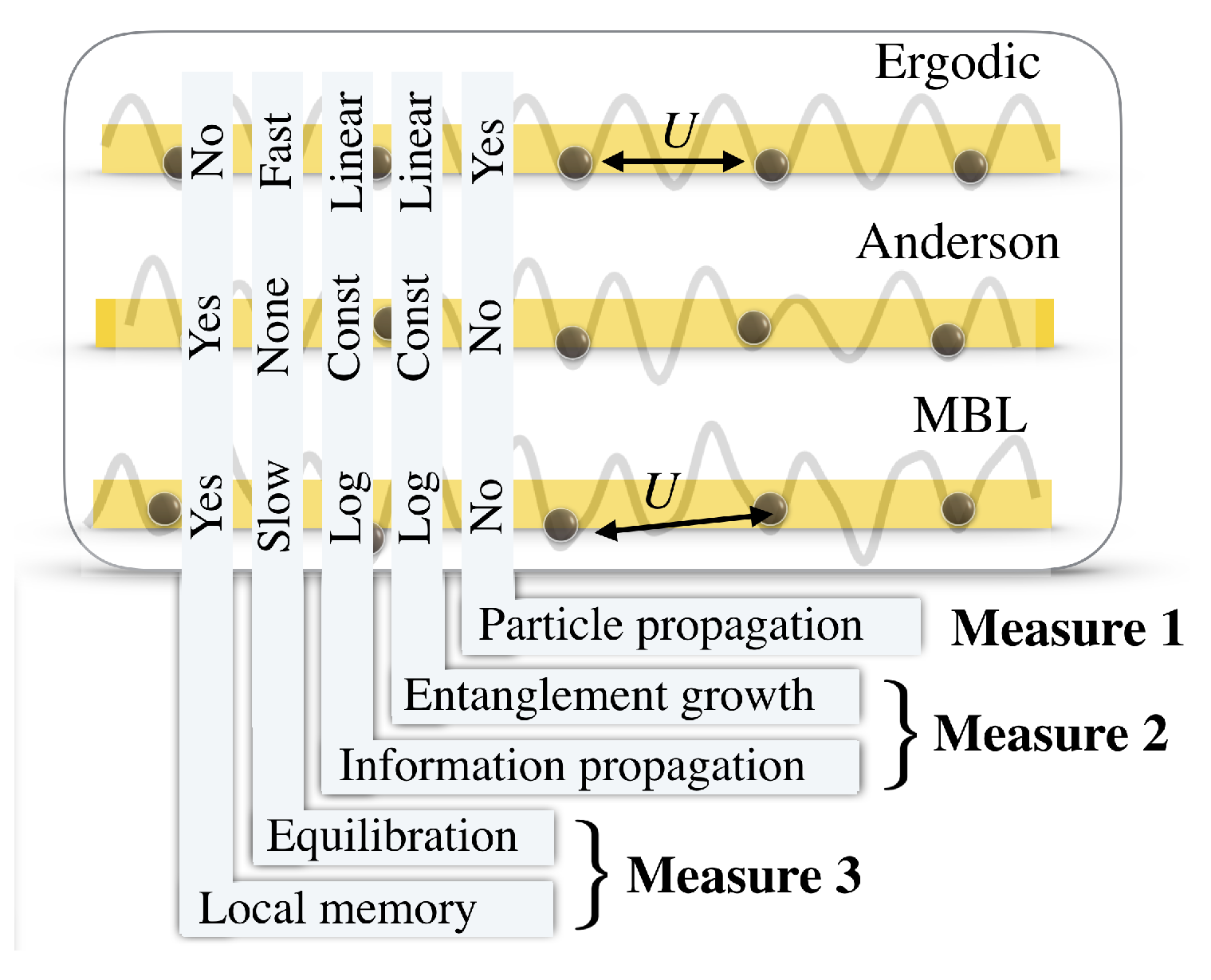
4. Phenomenology of Many-Body Localization

A fundamental characteristic of MBL is the presence of local constants of motion [3]. They are approximately local operators σ ˜ j z whose support is centered on lattice site j, but which nevertheless commute with the Hamiltonian, i.e., [ H , σ ˜ j ] = 0 . These operators are mainly supported on a region with diameter ξ , corresponding to the localization length scale of the system. In fact, in the MBL regime, the dynamics can be captured by a phenomenological model in terms of a set of mutually commuting quasi-local constants of motion,
H l Bit ( 2 ) = i μ i σ ˜ i z + j < i J i , j σ ˜ i z σ ˜ j z .
Such a Hamiltonian constitutes a second order approximation of what is known as the l-bit model [19,20,38] to exemplify the dynamics. Here, σ i z ˜ again denotes a quasi-local integral of motion centered on site i, μ i is a random onsite potential and the coupling strength J i , j between constants of motion is assumed to decay suitably fast in their distance d ( i , j ) . In particular, it is expected that the dynamics generated by the Hamiltonian defined in Equation (1) in the MBL regime corresponding to U = 2 and I > 7 can be well captured by the l-bit model.
This phenomenological model gives rise to a separation of time scales in the evolution into two regimes. Initially, there is a fast regime, where the evolution takes place mainly inside the support of each local constant of motion σ ˜ i z . Hence, for this time scale, transport is unconstrained and particles and energies can move freely inside the localization length. Correspondingly, information can spread ballistically. Beyond the localization length, the dynamics is dominated by the coupling of the constants of motion, given by the second term in Equation (3) [20]. The intuition is that this evolution does not facilitate particle or energy propagation, leading to a complete break-down of thermal and electric conductivity. Nevertheless, the couplings between distant constants of motion allow for the creation of correlations over arbitrary length scales given sufficient time. This dephasing mechanism in turn makes it possible to send information and yields an explanatory mechanism for the observed slow growth of entanglement [9,10,16], measured as the von Neumann entropy of the half chain of an infinite system S ( t ) = Θ ( log ( t ) ) (in Landau notation).
Mathematically, these two dynamical regimes are best distinguished by the effect of a local unitary excitation on distant measurements. More precisely, given a local measurement O A supported in a spatial region A and a unitary V B corresponding to a local excitation in a region B, we wish to bound the change in expectation value of O A ( t ) induced by the unitary excitation. This can be cast into a Lieb–Robinson bound [14,39] of the form
V B O A ( t ) V B O A ( t ) C ( A ) e μ ( d ( A , B ) v | t | ) I , t e μ d ( A , B ) II ,
where C ( A ) a constant depending on the support of O A . For the connection between different zero velocity Lieb–Robinson bounds and the necessity of a linear t-dependence in II, see Ref. [14]. Here, I corresponds to the ballistic regime and II captures the slower dephasing. In the context of optical lattices, local excitations seem difficult to implement. Hence, in the following, we focus on the observation of indirect effects on the dynamical evolution in MBL systems.

5. Feasible Witnesses

In the following, we demonstrate that local memory of initial conditions, slow spreading of correlations and equilibration of local densities provide clear measures to distinguish MBL systems from both the non-interacting Anderson insulators and the ergodic systems, i.e., those where local measurements, after a short relaxation time, can be captured by thermal ensembles. To carry out our analysis, we complement the intuitive guideline provided by the phenomenological l-bit model by a numerical tensor network TEBD simulation [40] (for details, see Appendix A). The chosen parameters for the simulation are a disorder strength of I = 8 and interaction strengths of U = 2 or U = 0 for the MBL and Anderson case, respectively. An overview of the measures and their capabilities is given in Figure 1. We begin by considering the influence of the suppression of particle propagation.

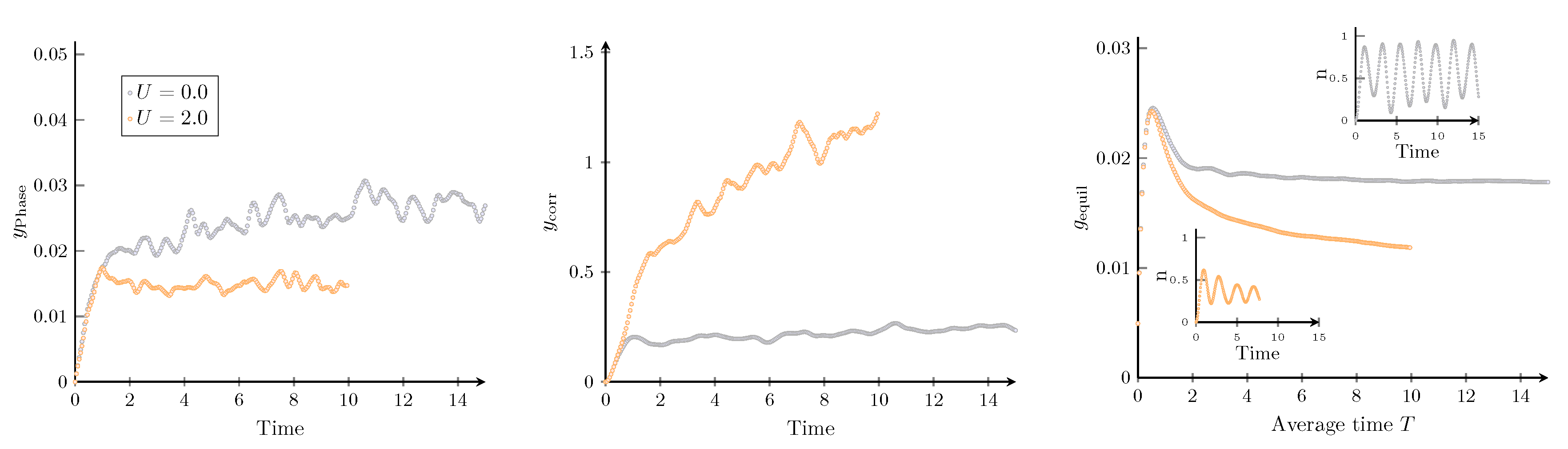
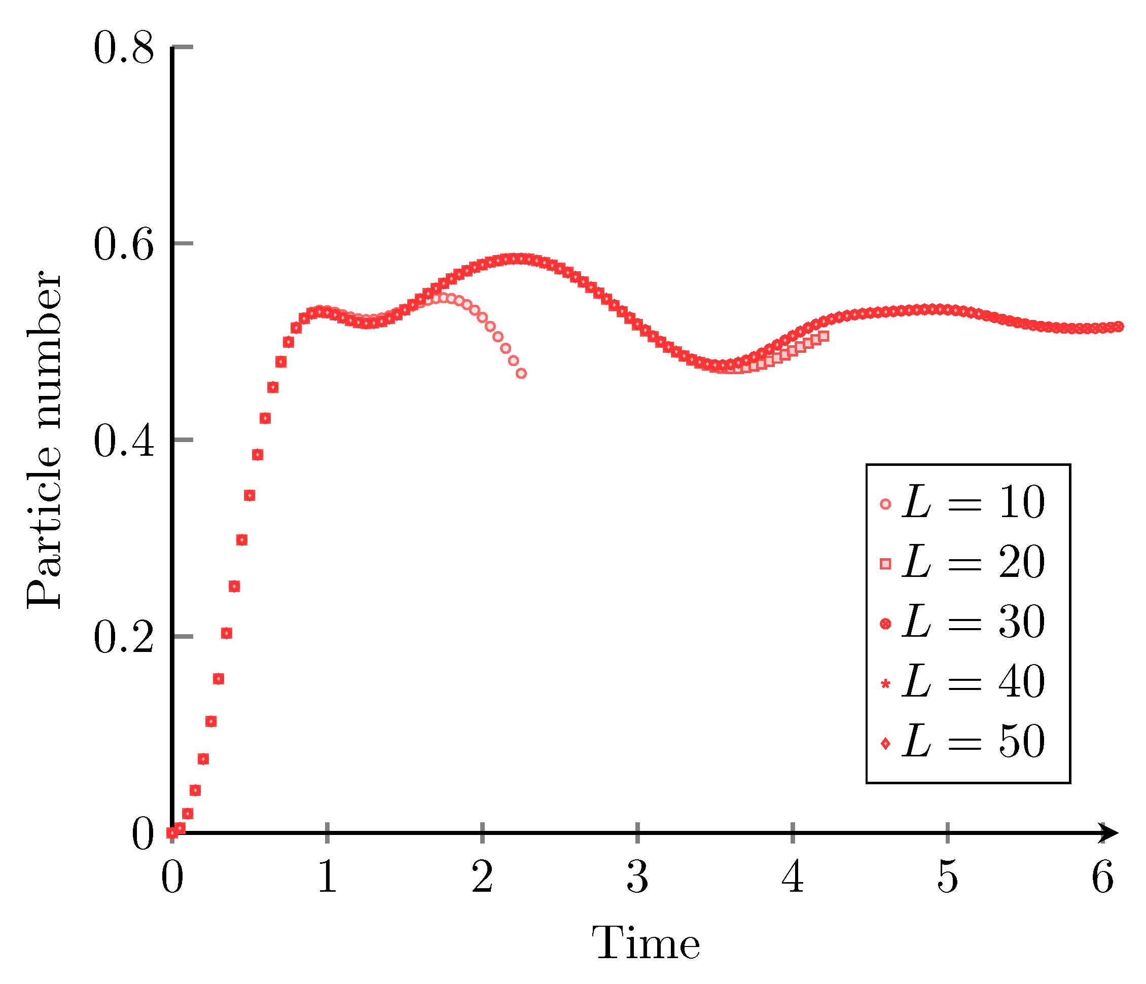
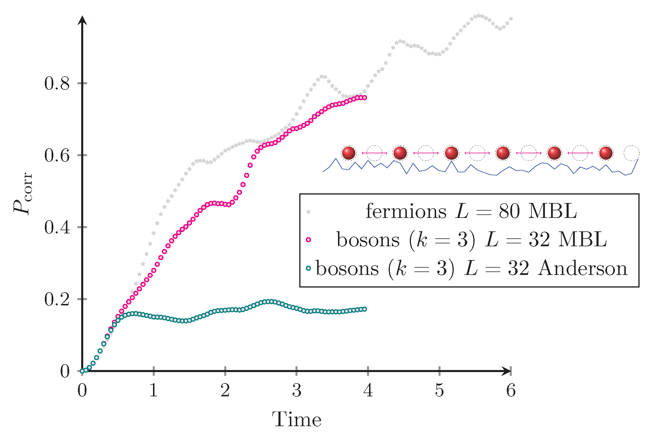
5.1. Absence of Particle Transport

A defining feature of localized systems is that independent of the interaction strength, particles and energies do not spread over the entire system, but remain confined to local regions. They merely redistribute inside the localization length, which can be extracted from the constants of motion. Therefore, even for long times, the particle density profile of an MBL system will not move to its thermal form, but rather retain some memory of its initial configuration. This gives rise to the following particle localization measure.
Measure 1 (Particle propagation and phase correlations).
We define the following measure y Phase ( t ) , which probes particle propagation for a system of length L
f Phase ( k , t ) : = f L / 2 ( t ) f L / 2 + k ( t ) ,
y Phase ( t ) = k f Phase ( k , t ) k 2 .
On an intuitive level, this measure directly probes the spread of particles, including weights based on the distance to the initial position L / 2 such that distant contributions are amplified.
Numerically, we find that y phase ( t ) initially shows a steep linear increase, indicative of the ergodic dynamics governed by the onsite term of Equation (3) (Figure 2). In the second regime, it fluctuates without visible growth, indicating a break-down of particle transport on length scales beyond the localization length. Thus, the length scale of the phase correlations established in the system can be bounded independent of time y Phase ( t ) = O ( 1 ) . For ergodic systems, where particles and energies spread ballistically, the measure would grow in an unconstrained fashion over time. Based on this insight, we deduce that time-of-flight images, while clearly distinguishing between localized and ergodic phase, are not useful for the distinction between interacting and non-interacting localized systems.
Again, more formally, this measure can be understood by considering the time evolution of the correlation matrix given by the matrix elements
γ j , k ( t ) : = f j ( t ) f k ( t ) ,
where f j f k = Tr ( f j ( t ) f k ( t ) ρ ) ) . For the non-interacting case of an Anderson insulator, this evolution is unitary γ ( t ) = U ( t ) γ ( 0 ) U ( t ) , where f j ( t ) = l U j , l ( t ) f l is the evolution of the fermionic mode operators. For an Anderson insulator, dynamical localization precisely corresponds to locality of the unitary evolution [41], meaning that the matrix elements of U are expected to decay exponentially | U j , k ( t ) | C e d ( j , k ) for some constant C with high probability [42].
In the case of interacting Hamiltonians that conserve the particle number, this time evolution can be captured in form of a quantum channel
γ ( t ) = l = 1 L 2 K l ( ρ 0 , t ) γ ( 0 ) K l ( ρ 0 , t ) ,
where the Kraus operators K l ( ρ 0 , t ) depend on the full initial state. As particle propagation in an MBL system is expected to also be localized, it is assumed that the individual Kraus operators obey | K j , k ( ρ 0 , t ) | C K e d ( j , k ) . Starting from an initial product state of the form in Equation (2), we obtain
γ z 1 , z 2 ( t ) = f z 1 ( t ) f z 2 ( t ) = j , l z 1 K ( ρ 0 , t ) j γ ( 0 ) j , l l K ( ρ 0 , t ) z 2 = j even C K 2 e d ( j , 0 ) d ( z 1 + j , z 2 ) .
This again results in a suppression with the distance between z 1 and z 2 , causing a saturation of the phase correlation measure f Phase ( k , t ) independent of time.

5.2. Slow Spreading of Information

While particles and energies remain confined in interacting localized systems, correlations are expected to show an unbounded increase over time [9,10], although slower than in the ergodic counterpart. In stark contrast, Anderson localized many-body systems will not build up any correlations that go beyond the localization length. To probe the spreading of correlations in the system, we focus on a quantity easily accessible in the context of optical lattices, using in-situ images for different evolution times. As it turns out, this kind of simple density–density correlator is already sufficient to separate Anderson localization from MBL systems.
Measure 2 (Logarithmic information propagation).
To examine the spatial spreading of density–density correlations, we define the quantity y Corr ( t ) ,
f Corr ( k , t ) : = | n L / 2 n L / 2 + k n L / 2 n L / 2 + k | ,
y Corr ( t ) : = k f Corr ( k , t ) k 2 .
y Corr is a direct indicator for the length scale over which density–density correlations are established without having to resort to assuming an explicit form, such as a decay in terms of an exponential function.
Comparable to the dynamics of the phase correlations, we numerically find a steep initial increase followed by a saturation for the non-interacting case (Figure 2). The MBL system, however, continues to build up density–density correlations for the times simulated. There is a transition in propagation speed, which we ascribe to the two dynamical regimes discussed before. Hence, we conclude that density–density correlations can be used to discriminate MBL from its non-interacting counterpart.
An intuitive explanation for the spread of density–density correlations despite spatial localization of particles is that, after exploring the localization length, the particles feel the presence of neighboring particles. Mediated by this interaction, the local movement of particles, governed by the respective constant of motion, becomes correlated, even over large distances. In contrast, in the Anderson insulator where constants of motion are completely decoupled, this communication cannot take place.
We can connect this intuitive explanation to the more rigorous setting of Lieb–Robinson bounds. In the Anderson insulator in one dimension, it is possible to prove that there exists a zero-velocity Lieb–Robinson bound, where the correlator on the left hand side of Equation (4) is bounded by a time independent factor e μ d ( A , B ) [44]. This means that the detectability of an excitation created in region A decreases exponentially with the distance to B. On the contrary, in the MBL regime we expect a logarithmic Lieb–Robinson cone of the form of Equation (4) II. Hence, an unbounded growth of correlations between distant regions is in principle possible, given sufficient time. Furthermore, we have shown that this built-up of correlations also happens on observable time scales, as can be seen from the evolution of density–density correlations captured by Measure 2.

5.3. Dephasing and Equilibration

It is also instructive to study the differences between the Anderson and MBL-regime with respect to their equilibration properties. Due to the interactions present, we expect equilibration of fluctuations to take place in MBL systems, whereas in Anderson insulators the effective subspaces explored by single particles remain small for all times and hence fluctuations remain large. This in turn implies that fluctuations of local expectation values die out in the interacting model, but persist in an Anderson insulator. This qualitative difference has already been identified as a signifier of interactions in a disordered system [21]. Here, we build upon this idea and propose to consider the average change rate of local expectation values in order to detect the decreasing fluctuations in the MBL phase.
Measure 3 (Density evolution: Equilibration of fluctuations).
We consider the expectation value f Eq ( t ) = n L / 2 ( t ) of a local density operator in the middle of the system. As a measure of local equilibration, we introduce the averaged rate of change of this density as a function of time T > 0
g Eq ( T ) : = 1 T 0 T d t | f Eq ( t ) | .
As laid out in Figure 2, again, this function over time indeed shows a remarkably smooth behavior that allows for the clear distinction between an Anderson localized system and its MBL counterpart in that, after a mutual increase, the Anderson system saturates at a constant value, whereas, in the MBL phase, g Eq shrinks successively.
If we again resort to the Lieb–Robinson bound picture, we find that in the Anderson case a local excitation is confined to a distinct spatial region given by the zero-velocity Lieb–Robinson bound introduced in the previous section. This implies that the effective subspace explored is constant and specifically, the excitation cannot build up long distance correlations and fluctuations remain large. This can also be seen from the results of Measure 2. If we now, however, turn to the interacting model, a local excitation will slowly explore larger and larger parts of the Hilbert space, leading to a slow, but persistent decrease of the fluctuations.

5.4. Present and Future Experimental Realizations

For an optical lattice architecture, the limitations of implementing the given measures are governed by the achievable repetition rate of the experiment and the quality of the initial state preparation. First, several repetitions are needed to get the expectation value of the measurements. Due to the disorder present in the system, it is furthermore necessary to repeat the first step with changing disorder to obtain a disorder averaged quantity. Lastly, since dynamics are in the focus of our measures, the described procedure needs to be carried out at any point in time. For linear quantities, such as Measure 1, Measure 3 or the imbalance, which is a measure of particle localization as well [21], the quantum average does in principle commute with the disorder average allowing for simultaneous averaging with fewer realizations. This is however not the case for non-linear quantities such as Measure 2. Here, the full procedure described above needs to be carried out. The repetition rates of optical lattices are on the order of seconds and leading experimentalists assured us that taking reliable data for all our measures is indeed feasible [45].
Recently, there was an impressive progress in measuring quantities very much related to the entanglement entropy in small one-dimensional optical lattices [46,47]. In both these works, quantities similar to to our Measure 2 are used as well. In Ref. [47], the authors defined a quantity called transport distance which basically coincides with our Measure 2. The difference being that their scaling function is only linear instead of quadratic. However, they dis not employ this measure to show the many-body correlations in these systems. Rather, they calculated the number and configurational entanglement [46]. The system sizes used are very restricted, possibly due to the complicated procedure of obtaining these entropies.
We think that an implementation of Measure 2 or Measure 3 might complement these results nicely by overcoming these problems and hence being applicable also for larger systems and potentially also higher dimensional systems, where the fate of MBL is still debated.

6. Conclusions and Outlook

In this work, we proposed an operational procedure for distinguishing MBL phases building upon realistic measurements, which can be performed in the realm of optical lattices with present technology. Utilizing a phenomenological model and the concept of Lieb–Robinson bounds, we explained the effects numerically investigated employing tensor network methods. The equilibration of local observables allows for the distinction of Anderson and MBL localized models. Density–density correlations allow for the same information bit extraction, while also reproducing the expected phenomenology. Further investigating this quantity might yield information about the localization length via the duration of the first evolution regime.
Phase correlations, which are directly connected to ToF imaging, cannot detect interactions in a localized system due to their correspondence to particle transport. There is yet other information the ToF reveals: One can also lower bound the spatial entanglement of bosons in optical lattices [48], building upon the ideas of constructing quantitative entanglement witnesses [25,26,27], a notion of multi-partite entanglement M ( t ) detecting a deviation from a best separable approximation, as M ( t ) max ( 0 , n n ( q ) / | w ^ 0 ( q ) | 2 ) for all q. This quantity detects a reasonable notion of multi-particle entanglement, which is yet different from the bi-partite entanglement discussed above. Since this measure is only onsite local, we would expect that it cannot distinguish the long-range correlations of an interacting disordered model from the dynamics inside the constant of motion. This further motivates the quest to engineer appropriate entanglement witnesses both accessible in optical lattice architectures as well as probing key features of MBL, a quest that is in turn expected to contribute to our understanding of MBL as such.

Author Contributions

Conceptualization: M.F., W.B., A.H.W. and J.E. Investigation: M.G. and M.F. Writing—Original Draft Preparation: M.G. and M.F. Writing—Review and Editing: A.H.W. and J.E. Validation: A.H.W. and J.E. Visualization: M.F. and J.E. Supervision: J.E. Project Administration: J.E. Funding Acquisition: J.E.

Funding

This research was funded by the DFG grant number FOR2724, CRC 183, EI 519/14-1, EI 519/7-1, EI 519/15-1, the European Commission grant number AQUS, SIQS, RAQUEL, the Templeton Foundation, the ERC grant number TAQ, the European Union’s Horizon 2020 research and innovation programme under grant agreement No. 817482 (PASQuanS).

Acknowledgments

We warmly thank A. Rubio Abadal, U. Schneider, C. Gross, I. Bloch, A. Scardicchio, and R. Vasseur for discussions. Note added: This work was first submitted as a preprint as a blueprint for a joint experimental-theoretical effort in progress. We now decided to properly publish this work in Quantum Reports as a scientific venue that is sympathetic to preprints. We insist that this work is still timely and guiding present and future experiments.

Conflicts of Interest

The authors declare no conflict of interest.

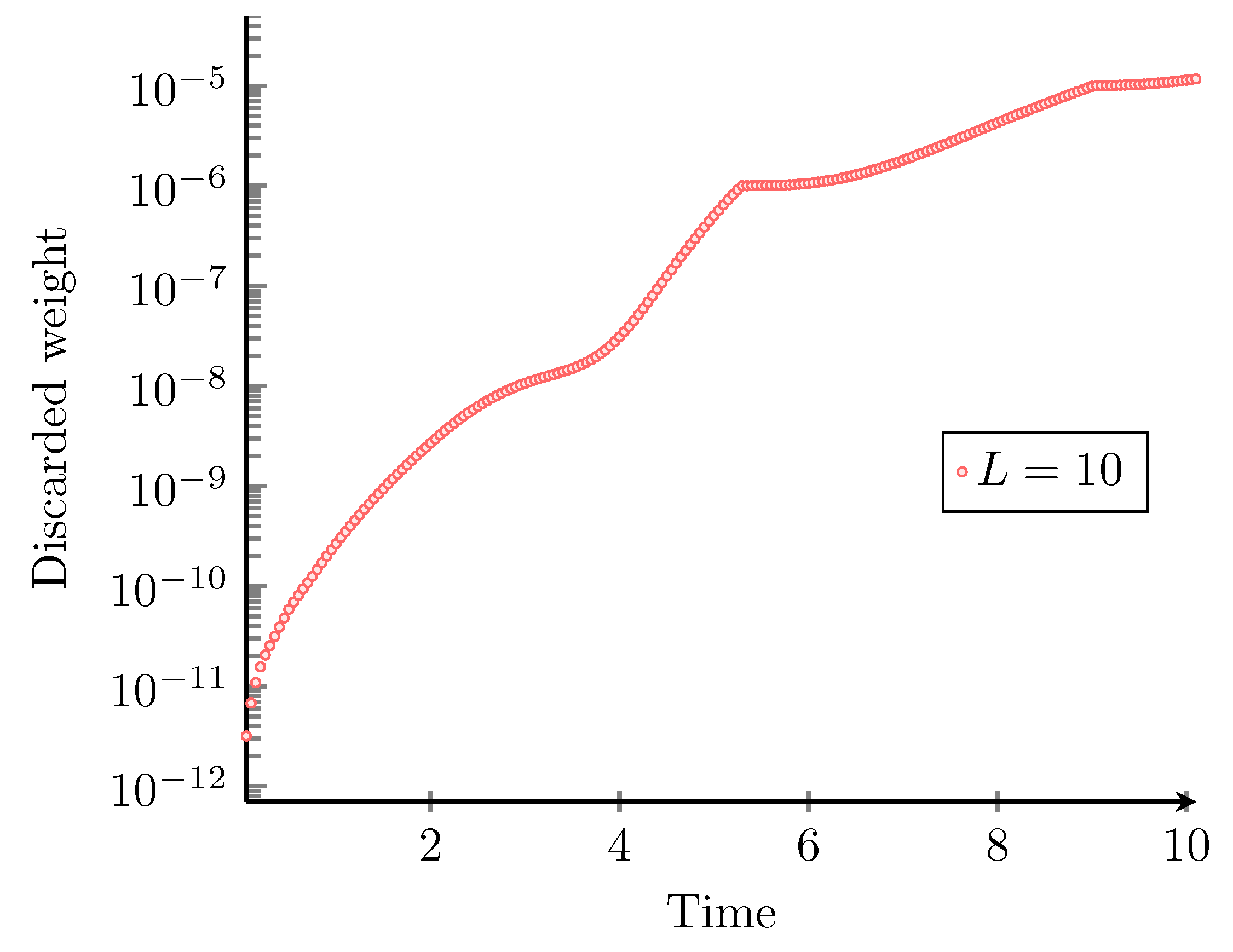
Appendix A. Numerical Details

In this appendix, we present the details of our numerical simulations. Our results mainly rely on a matrix-product state simulation based on a TEBD code [43], thus an instance of a tensor network state simulation. To corroborate the results, we further employ an exact diagonalization code [49] that uses the particle number symmetry and keeps track of the time evolution with a Runge–Kutta integration scheme. For the non-interacting case, further checks are performed by an explicit simulation of the dynamical evolution of the covariance matrix, which takes a particularly easy form in this case.
For short times and the system sizes that can be achieved with exact diagonalization, the codes agree up to a negligible error, thus also demonstrating that the chosen step size in the fifth-order Trotter decomposition used in TEBD [43] of τ step does not produce significant errors. This leaves only two potential error sources: the fact that numerics necessarily simulate a finite system and the possibility of discarded weights accumulating over time.
Performing a finite size scaling, we find that comparably small systems are already indistinguishable from the thermodynamic limit for the quantities considered here (see Figure A1). This is in agreement with the very slow growth of Lieb–Robinson cones expected in these disordered systems. To be on the safe side, we have nevertheless carried out our numerical analysis on systems with L = 80 sites and open boundary conditions.
Having demonstrated that the considered system size is indistinguishable from the thermodynamic limit only leaves the discarded weight as potential error source (see Figure A2). The time evolution of this quantity, which is directly connected to spatial entanglement entropies, depends strongly on the chosen disorder realization. To keep this discarded weight small enough, we increase the bond dimension in the simulation in a three-step procedure up to d Bond = 350 , which is sufficient to guarantee a discarded weight smaller than 2 × 10 5 for all disorder realizations.
Figure A1. Finite size scaling for the evolution of particle density in the middle of the chain for a typical disorder realization. For L = 10 , 20 , an exact diagonalization code was used. The other system sizes are simulated with a TEBD code [43].
Quantumrep 01 00006 g0a1
Figure A2. Evolution of the discarded weight. This plot varies strongly depending on the chosen disorder realization. From the 100 realizations used for the averaged plots, the realization with the largest discarded weights is shown here.
Quantumrep 01 00006 g0a2

Appendix B. Bosonic Model with On-Site Interactions

In this appendix, we show additional simulation data for a measure similar to Measure 2 for a related model that is used in some of the experimental realizations of MBL. This is the disordered Bose–Hubbard model with on-site interactions given by
H = j b j b j + 1 + h . c . + j w j n j + U j n j n j ,
where b j denotes a bosonic operator on site j, n j = b j b j is the local particle number operator and, again, we draw the w j from the uniform distribution on the interval [ I , I ] . In contrast to the fermionic variant in the main text, we here need to restrict the local Hilbert space to be able to perform numerics. We restrict the local particle number to k = 3 particles per site, but also make sure that enlarging the local dimension would not change our results qualitatively. Moreover, our initial state is again an MIS state as defined in Equation (2), featuring an average particle number of 0.5 per site. The measure we employ for bosons is identical to Measure 2 with the exception that the number operators were replaced by parity operators.
Measure 4 (Logarithmic information propagation).
To examine the spatial spreading of parity–parity correlations, we define the quantity P Corr ( t ) ,
f Corr ( k , t ) : = | p L / 2 p L / 2 + k p L / 2 p L / 2 + k | ,
P Corr ( t ) : = k f Corr ( k , t ) k 2 ,
where p is the local parity operator.
In Figure A3, we show Measure 4 for the Anderson ( U = 0 ) and MBL ( U = 2 ) case. Similar to the main text, we find that, in the non-interacting case, the measure saturates after few tunneling times. In contrast, for the interacting model, we found that the measure grew in comparable fashion to the fermionic counterpart (grey stars). This suggests that the correlation measure can be employed in similar models as well.
Figure A3. Plotted are the results of a TEBD simulation of the dynamical evolution of the parity–parity correlations P corr . The initial state ψ is again found in Equation (2) under the Hamiltonian in Equation (A1) for the case of an Anderson insulator with U = 0 and MBL with U = 2 . We compared the results of the fermionic MBL setting and the bosonic MBL and Anderson setting with a local Hilbert space dimension truncation k = 3 . Every data point corresponds to an average of over 100 realizations.
Quantumrep 01 00006 g0a3

References

  1. Basko, D.M.; Aleiner, I.L.; Altshuler, B.L. Metal-insulator transition in a weakly interacting many-electron system with localized single-particle states. Ann. Phys. 2006, 321, 1126. [Google Scholar] [CrossRef]
  2. Anderson, P.W. Absence of Diffusion in Certain Random Lattices. Phys. Rev. 1958, 109, 1492. [Google Scholar] [CrossRef]
  3. Nandkishore, R.; Huse, D.A. Many-Body Localization and Thermalization in Quantum Statistical Mechanics. Ann. Rev. Cond. Mat. Phys. 2015, 6, 15–38. [Google Scholar] [CrossRef] [Green Version]
  4. Pal, A.; Huse, D.A. The many-body localization transition. Phys. Rev. B 2010, 82, 174411. [Google Scholar] [CrossRef]
  5. Oganesyan, V.; Huse, D.A. Localization of interacting fermions at high temperature. Phys. Rev. B 2007, 75, 155111. [Google Scholar] [CrossRef] [Green Version]
  6. Polkovnikov, A.; Sengupta, K.; Silva, A.; Vengalattore, M. Non-equilibrium dynamics of closed interacting quantum systems. Rev. Mod. Phys. 2011, 83, 863. [Google Scholar] [CrossRef]
  7. Eisert, J.; Friesdorf, M.; Gogolin, C. Quantum many-body systems out of equilibrium. Nat. Phys. 2015, 11, 124–130. [Google Scholar] [CrossRef] [Green Version]
  8. Gogolin, C.; Eisert, J. Equilibration, thermalisation, and the emergence of statistical mechanics in closed quantum systems. Rep. Prog. Phys. 2016, 79, 056001. [Google Scholar] [CrossRef] [Green Version]
  9. Znidaric, M.; Prosen, T.; Prelovsek, P. Many-body localization in the Heisenberg XXZ magnet in a random field. Phys. Rev. B 2008, 77, 064426. [Google Scholar] [CrossRef]
  10. Bardarson, J.H.; Pollmann, F.; Moore, J.E. Unbounded Growth of Entanglement in Models of Many-Body Localization. Phys. Rev. Lett. 2012, 109, 017202. [Google Scholar] [CrossRef] [Green Version]
  11. Goold, J.; Clark, S.R.; Gogolin, C.; Eisert, J.; Scardicchio, A.; Silva, A. Total correlations of the diagonal ensemble herald the many-body localisation transition. Phys. Rev. B 2015, 92, 180202(R). [Google Scholar] [CrossRef]
  12. Eisert, J.; Cramer, M.; Plenio, M.B. Area laws for the entanglement entropy. Rev. Mod. Phys. 2010, 82, 277. [Google Scholar] [CrossRef]
  13. Bauer, B.; Nayak, C. Area laws in a many-body localised state and its implications for topological order. J. Stat. Mech. 2013, 2013, P09005. [Google Scholar] [CrossRef]
  14. Friesdorf, M.; Werner, A.H.; Brown, W.; Scholz, V.B.; Eisert, J. Many-body localisation implies that eigenvectors are matrix-product states. Phys. Rev. Lett. 2015, 114, 170505. [Google Scholar] [CrossRef] [PubMed]
  15. Srednicki, M. Chaos and quantum thermalization. Phys. Rev. E 1994, 50, 888–901. [Google Scholar] [CrossRef] [Green Version]
  16. Kim, I.H.; Chandran, A.; Abanin, D.A. Local integrals of motion and the logarithmic light cone in many-body localised systems. Phys. Rev. B 2015, 91, 085425. [Google Scholar]
  17. Chandran, A.; Carrasquilla, J.; Kim, I.H.; Abanin, D.A.; Vidal, G. Spectral tensor networks for many-body localisation. Phys. Rev. B 2015, 92, 024201. [Google Scholar] [CrossRef]
  18. Friesdorf, M.; Werner, A.H.; Goihl, M.; Eisert, J.; Brown, W. Local constants of motion imply transport. New J. Phys. 2015, 17, 113054. [Google Scholar] [CrossRef]
  19. Serbyn, M.; Papić, Z.; Abanin, D.A. Local Conservation Laws and the Structure of the Many-Body Localized States. Phys. Rev. Lett. 2013, 111, 127201. [Google Scholar] [CrossRef] [PubMed] [Green Version]
  20. Huse, D.A.; Nandkishore, R.; Oganesyan, V. Phenomenology of fully many-body-localized systems. Phys. Rev. B 2014, 90, 174202. [Google Scholar] [CrossRef] [Green Version]
  21. Schreiber, M.; Hodgman, S.S.; Bordia, P.; Lüschen, H.P.; Fischer, M.H.; Vosk, R.; Altman, E.; Schneider, U.; Bloch, I. Observation of many-body localization of interacting fermions in a quasi-random optical lattice. Science 2015, 349, 842. [Google Scholar] [CrossRef] [PubMed]
  22. Bordia, P.; Lüschen, H.P.; Hodgman, S.S.; Schreiber, M.; Bloch, I.; Schneider, U. Coupling Identical one-dimensional Many-Body Localized Systems. Phys. Rev. Lett. 2016, 116, 140401. [Google Scholar] [CrossRef] [PubMed]
  23. Wiersma, D.S.; Bartolini, P.; Lagendijk, A.; Righini, R. Localization of light in a disordered medium. Nature 1997, 390, 671–673. [Google Scholar] [CrossRef]
  24. Bloch, I.; Dalibard, J.; Nascimbene, S. Quantum simulations with ultracold quantum gases. Nat. Phys. 2012, 8, 267. [Google Scholar] [CrossRef]
  25. Eisert, J.; Brandao, F.G.; Audenaert, K.M. Quantitative entanglement witnesses. New J. Phys. 2007, 9, 46. [Google Scholar] [CrossRef]
  26. Audenaert, K.M.R.; Plenio, M.B. When are correlations quantum? New J. Phys. 2006, 8, 266. [Google Scholar] [CrossRef]
  27. Guehne, O.; Reimpell, M.; Werner, R.F. Estimating entanglement measures in experiments. Phys. Rev. Lett. 2007, 98, 110502. [Google Scholar] [CrossRef]
  28. Gring, M.; Kuhnert, M.; Langen, T.; Kitagawa, T.; Rauer, B.; Schreitl, M.; Mazets, I.; Smith, D.A.; Demler, E.; Schmiedmayer, J. Relaxation and Prethermalization in an Isolated Quantum System. Science 2012, 337, 1318. [Google Scholar] [CrossRef]
  29. Steffens, A.; Friesdorf, M.; Langen, T.; Rauer, B.; Schweigler, T.; Hübener, R.; Schmiedmayer, J.; Riofrio, C.A.; Eisert, J. Towards experimental quantum field tomography with ultracold atoms. Nat. Commun. 2015, 6, 7663. [Google Scholar] [CrossRef]
  30. Luitz, D.J.; Laflorencie, N.; Alet, F. Many-body localisation edge in the random-field Heisenberg chain. Phys. Rev. B 2015, 91, 081103. [Google Scholar] [CrossRef]
  31. Singh, R.; Bardarson, J.H.; Pollmann, F. Signatures of the many-body localization transition in the dynamics of entanglement and bipartite fluctuations. New J. Phys. 2016, 18, 023046. [Google Scholar] [CrossRef] [Green Version]
  32. Serbyn, M.; Papić, Z.; Abanin, D.A. Criterion for many-body localization-delocalization phase transition. Phys. Rev. X 2015, 5, 041047. [Google Scholar] [CrossRef]
  33. Serbyn, M.; Knap, M.; Gopalakrishnan, S.; Papic, Z.; Yao, N.Y.; Laumann, C.R.; Abanin, D.A.; Lukin, M.D.; Demler, E.A. Interferometric Probes of Many-Body Localization. Phys. Rev. Lett. 2014, 113, 147204. [Google Scholar] [CrossRef] [PubMed]
  34. Roy, D.; Singh, R.; Moessner, R. Probing many-body localisation by spin noise spectroscopy. Phys. Rev. B 2015, 92, 180205. [Google Scholar] [CrossRef]
  35. Vasseur, R.; Parameswaran, S.A.; Moore, J.E. Quantum revivals and many-body localization. Phys. Rev. B 2015, 91, 140202. [Google Scholar] [CrossRef] [Green Version]
  36. Choi, J.Y.; Hild, S.; Zeiher, J.; Schauß, P.; Rubio-Abadal, A.; Yefsah, T.; Khemani, V.; Huse, D.A.; Bloch, I.; Gross, C. Exploring the many-body localization transition in two dimensions. Science 2016, 352, 1547–1552. [Google Scholar] [CrossRef] [Green Version]
  37. Trotzky, S.; Chen, Y.A.; Flesch, A.; McCulloch, I.P.; Schollwoeck, U.; Eisert, J.; Bloch, I. Probing the relaxation towards equilibrium in an isolated strongly correlated one-dimensional Bose gas. Nat. Phys. 2012, 8, 325. [Google Scholar] [CrossRef]
  38. Ros, V.; Müller, M.; Scardicchio, A. Integrals of motion in the many-body localized phase. Nucl. Phys. B 2015, 891, 420–465. [Google Scholar] [CrossRef] [Green Version]
  39. Lieb, E.H.; Robinson, D.W. The finite group velocity of quantum spin systems. Commun. Math. Phys. 1972, 28, 251–257. [Google Scholar] [CrossRef]
  40. Daley, A.J.; Kollath, C.; Schollwoeck, U.; Vidal, G. Time-dependent density-matrix renormalization- group using adaptive effective Hilbert spaces. J. Stat. Mech. 2004, 2004, P04005. [Google Scholar] [CrossRef]
  41. Kirsch, W. An invitation to random Schroedinger operators. arXiv 2007, arXiv:0709.3707. [Google Scholar]
  42. Germinet, F.; Klein, A. Bootstrap multi-scale analysis and localization in random media. Commun. Math. Phys. 2001, 222, 415. [Google Scholar] [CrossRef]
  43. Wall, M.L.; Carr, L.D. Open Source TEBD. 2013. Available online: http://physics.mines.edu/downloads/software/tebd(2009) (accessed on 12 June 2019).
  44. Burrell, C.K.; Eisert, J.; Osborne, T.J. Information propagation through quantum chains with fluctuating disorder. Phys. Rev. A 2009, 80, 052319. [Google Scholar] [CrossRef] [Green Version]
  45. Gross, C.; Bloch, I.; (Max-Planck-Institut für Quantenoptik, Garching, Germany). Personal communication, 2018.
  46. Lukin, A.; Rispoli, M.; Schittko, R.; Tai, M.E.; Kaufman, A.M.; Choi, S.; Khemani, V.; Leonard, J.; Greiner, M. Probing entanglement in a many-body-localized system. arXiv 2018, arXiv:1805.09819. [Google Scholar]
  47. Rispoli, M.; Lukin, A.; Schittko, R.; Kim, S.; Tai, M.E.; Léonard, J.; Greiner, M. Quantum critical behavior at the many-body-localization transition. arXiv 2018, arXiv:1812.06959. [Google Scholar]
  48. Cramer, M.; Bernard, A.; Fabbri, N.; Fallani, L.; Fort, C.; Rosi, S.; Caruso, F.; Inguscio, M.; Plenio, M. Spatial entanglement of bosons in optical lattices. Nat. Commun. 2013, 4, 2161. [Google Scholar] [CrossRef]
  49. Jones, E.; Oliphant, T.; Peterson, P. SciPy: Open Source Scientific Tools for Python; ResearchGate: Berlin, Germany, 2001. [Google Scholar]
Figure 1. An overview over the dynamical behavior of MBL systems versus their ergodic and thermalizing and Anderson localized counterparts. Measure 1 detects particle propagation and phase correlations and can be implemented using time-of-flight imaging. Measure 2 and Measure 3 utilize in-situ imaging to observe density–density correlations and equilibration behavior.
Quantumrep 01 00006 g001
Figure 2. Plotted are the results of a TEBD simulation [43] of the dynamical evolution of the initial state ψ from Equation (2) under the Hamiltonian in Equation (1) for the case of an Anderson insulators with U = 0 and MBL with U = 2 . The disorder strength is I = 8 . The three plots are averaged over 100 disorder realizations. (Left) Shown is the time evolution of y Phase defined in Measure 1 demonstrating that the phase correlation behavior saturates both for MBL and Anderson localization. (Middle) The plot shows the dynamical evolution of y Corr defined in Measure 2. Information propagation is fully suppressed in an Anderson insulator, resulting in a saturation of this quantity. In contrast, correlations continue to spread in the MBL system beyond all bounds, giving rise to a remarkably strong signal feasible to be detected in experiments. (Right) Shown are the averaged fluctuations g Eq defined in Measure 3 as a function of the time T over which the average is performed. The insets show the time evolution of the particle density at the position L / 2 , which enters the calculation of g Eq for one disorder realization, which is identical for the MBL and Anderson localized model. As the insets also show, the local fluctuations continue indefinitely for the Anderson insulator, corresponding to a saturation of g Eq , while the MBL system equilibrates and g Eq continues to decrease accordingly.
Quantumrep 01 00006 g002

