The Unsteady Aerodynamic Response of the DrivAer Fastback to Longitudinal Acceleration and Deceleration

Abstract

This study examines the aerodynamic response of a DrivAer fastback model subjected to longitudinal acceleration and deceleration using a time-varying inlet-velocity approach. The accelerating, non-accelerating, and decelerating cases are compared at a common reference velocity to isolate the influence of acceleration history from the effect of instantaneous flow speed. The results show that the DrivAer fastback produces different drag, lift, lift-balance, and wake-field behavior depending on whether the flow is accelerating or decelerating. In comparison to the non-accelerating case, drag decreases during deceleration and increases during acceleration, while the lift distribution also shifts between the front and rear of the vehicle. Flow-field comparisons show that the changes in aerodynamic force are linked to altered flow behavior around the rear-glass, decklid, and wake regions. These results suggest that a quasi-steady interpretation based only on instantaneous velocity is not sufficient to describe the aerodynamic response of road-vehicle geometry under longitudinal acceleration and deceleration.

1. Introduction

Despite the inherently unsteady nature of real-world driving, most road-vehicle aerodynamic studies, whether focused on idealized ground vehicles, production passenger cars, or racecars, are conducted under the simplifying assumption of a steady mean free-stream velocity. This assumption is widely used in studies of isolated-vehicle aerodynamics, vehicle-passing maneuvers, yaw and pitch effects, and coupled aerodynamic and thermal performance optimization [1,2,3,4,5,6]. The steady-flow framework has proven valuable because it enables the dominant aerodynamic characteristics of a vehicle, including drag, lift, surface-pressure distributions, and wake topology, to be examined under controlled and repeatable conditions. Early investigations of simplified ground-vehicle geometries, most notably the Ahmed body, demonstrated that pressure drag is governed largely by rear-end flow separation and the associated low-pressure wake region [1]. Subsequent studies employing standardized geometries, such as the DrivAer model, extended this approach to more representative passenger-vehicle configurations [2,7,8,9]. Nevertheless, even under nominally steady inflow conditions, accurate prediction of the separated wake remains difficult for practical vehicle geometries. This challenge is particularly pronounced for lower-fidelity turbulence closures, including steady Reynolds-averaged Navier–Stokes (RANS) models, which may not adequately resolve the inherently unsteady coherent structures that develop in the rear wake [2,8].

In real driving environments, the flow approaching a vehicle is rarely perfectly steady. It can change due to atmospheric turbulence, gusts, crosswinds, roadside features, or disturbances from nearby traffic. Several recent studies have, therefore, examined vehicle models subjected to unsteady inflow conditions. In these cases, the incoming flow is not treated as steady; instead, it may include time-dependent velocity components, changing flow direction, or other transient changes in the oncoming flow [10,11]. These studies have shown that aerodynamic loads can differ significantly from quasi-steady predictions, which assume the flow responds like a sequence of steady conditions [10,11,12,13,14,15,16].

The turbulence state of the incoming free stream, including turbulence intensity, can influence bluff-body and vehicle wake behavior; c.f. [17,18,19], to cite but a few. Although these studies represent many operating conditions, they do not fully describe how the airflow and resulting aerodynamic characteristics change when the vehicle itself is accelerating or decelerating. This distinction is important because longitudinal acceleration and deceleration produce a time-varying relative flow speed even when the incoming flow direction remains aligned with the vehicle. These conditions are important for passenger vehicles during transient events such as merging, passing, emergency braking, and collision avoidance. They also provide a useful point of comparison to higher-performance applications, where rapid speed changes occur frequently and stability limits can be smaller. These factors make acceleration- and deceleration-driven effects important for extending aerodynamic research toward more realistic operating conditions.

Changes in the incoming flow can affect separation, wake formation, and aerodynamic loads, meaning that the wake is not controlled only by the mean free-stream velocity. Related unsteady-flow studies support this idea. Passmore et al. [20] experimentally studied simplified vehicle bodies under unsteady wind-tunnel conditions and showed that the transient aerodynamic response can differ from quasi-steady predictions. Zhang et al. [21] showed that a sinusoidal inflow velocity can affect bluff-body wake behavior, with the inflow period influencing transitions between bistable wake states. The wake behind a bluff body can settle into one of two preferred flow patterns, and it can switch from one to the other. These studies show that separated wakes are sensitive to upstream-flow unsteadiness, which motivates the present focus on how longitudinal acceleration and deceleration affect the DrivAer wake at a common reference velocity.

The broader fluid-mechanics literature supports the idea that acceleration and deceleration can alter aerodynamic behavior relative to steady motion at the same instantaneous speed. Roohani and Skews [22] showed that aerofoils undergoing acceleration or deceleration in compressible flow experienced aerodynamic forces and moments that differed from steady-state values at the same Mach number. Theoretical work has also shown that accelerating-body aerodynamics can be described using a moving, non-inertial reference frame, where additional terms appear in the governing equations to account for acceleration effects [23]. More recent bluff-body studies with transient acceleration and deceleration have shown that these conditions can affect quantities such as surface pressure, wake development, vortex shedding, and aerodynamic forces [24,25,26]. Although these studies are not all road-vehicle specific, they support the expectation that separated bluff-body flows can show different force and wake behavior during acceleration compared with steady-flow conditions; not that deceleration can be viewed as the negative acceleration.

Prior work by Peters and Uddin [27], conducted on a simplified bluff body, developed a method for isolating acceleration-dependent aerodynamic effects. In their work, longitudinal acceleration and deceleration were imposed through a periodic inlet velocity applied to a channel-mounted square cylinder. This configuration generated repeatable accelerating and decelerating phases and allowed flow quantities to be compared at a common reference speed. Their results showed clear differences in drag, near-body flow structures, wake dynamics, Kármán vortex-street behavior, and vorticity production between accelerating, decelerating, and steady inlet conditions. These findings demonstrate that acceleration/deceleration history can influence bluff-body aerodynamic behavior even when the instantaneous reference speed is the same.

To interpret the additional force contribution associated with acceleration, Peters and Uddin adopted the framework of Morison [28]. In this formulation, the instantaneous streamwise force is decomposed into two components: an inertia-related term associated with fluid acceleration and a conventional drag term proportional to the square of the velocity. This separation makes it possible to compare the acceleration- and deceleration-related force contribution across different flow conditions:

$$F_x\left(t\right)=\rho \mathbb{V}{C}_M{\dot{V}}_x+{\displaystyle \frac{1}{2}}{C}_D\rho A{V}_x^2$$

(1)

where $\rho$ is the fluid density, $\mathbb{V}$ is the volume of the test body, $C_M$ is the coefficient of mass, ${\dot{V}}_x$ is the longitudinal acceleration rate of the fluid or test body, A is the frontal area of the test body, $C_D$ is the drag coefficient, and $V_x$ is the velocity of the fluid or test body in stream-wise direction (x).

The Morison formulation provides one way to describe acceleration-related force contributions. Another important feature of unsteady vehicle aerodynamics is that the wake itself may respond with a time delay. Theissen et al. [10] provide a clear example of this delayed wake response. In their experiment, a realistic 50%-scale vehicle model was oscillated about its vertical axis to create time-varying oncoming-flow conditions at representative Reynolds and Strouhal numbers. Their results showed that the unsteady aerodynamic loads differed significantly from the quasi-steady loads. In particular, the unsteady yaw moment exceeded the quasi-steady approximation by approximately 80%. Theissen et al. also found a noticeable time delay in the wake response, with $\Delta t/T\approx 0.15$. This delayed wake response was identified as a main reason that unsteady loads do not match quasi-steady predictions. Wojciak et al. [11] further reinforced this observation using a 50%-scale generic notchback model to reproduce time-dependent crosswind conditions. Their results showed again that unsteady loads can differ significantly from quasi-steady estimates, and that the unsteady yaw moment can exceed the maximum value observed under steady-flow conditions. The unsteady load behavior was linked to the crosswind wake structure, which includes a high-speed region near the leeward side and a pair of counter-rotating vortices. As the effective crosswind condition changes, this wake structure responds with a time delay, producing phase-shifted pressure changes at the rear of the vehicle. This produces a larger unsteady yaw-moment response, while the side force and roll moment can be reduced relative to the quasi-steady case.

Together, the simplified acceleration work and the unsteady vehicle studies show that changing flow conditions can strongly affect wakes and aerodynamic loads. The next step is to apply that acceleration framework to a passenger-vehicle shape, but this extension is not straightforward. A passenger vehicle includes three-dimensional separation, ground effect, underbody flow, rear-glass separation, rear-end wake development, and pressure interactions that are not fully represented by a channel-mounted square cylinder. Therefore, the aerodynamic response of a full vehicle under longitudinal acceleration and deceleration cannot be assumed to follow directly from simplified bluff-body behavior. A standardized vehicle geometry is needed to connect the acceleration-aerodynamics framework to a more representative road-vehicle flow field.

Motivated by these findings, the present study examines the effects of longitudinal acceleration and deceleration on the DrivAer fastback configuration under a time-varying inlet condition. The DrivAer fastback is used because it provides a realistic and standardized road-vehicle geometry while retaining the separated-flow behavior and wake complexity important to passenger-vehicle aerodynamics [2,7]. By comparing accelerating, steady, and decelerating flow conditions at a common reference speed, this work examines how acceleration history changes aerodynamic forces, lift balance, and wake development. In doing so, this study connects the simplified bluff-body acceleration framework to a standardized passenger-vehicle configuration.

The present work has direct relevance to the prediction and control of passenger-vehicle response during rapidly changing operating conditions. Large longitudinal accelerations commonly occur during emergency braking and collision-avoidance maneuvers, where aerodynamic loads may evolve differently from those predicted under steady-state assumptions. For current driver-in-the-loop systems, this knowledge can improve the fidelity of vehicle-dynamics and braking simulations used to evaluate stability, control authority, and stopping performance. Its importance is expected to increase further with the development of automated and autonomous vehicles, for which predictive control algorithms rely on accurate transient models to estimate vehicle response and support real-time collision mitigation. The results may also inform the modeling of rapidly developing or decaying crosswind gusts in lane-keeping and stability-control applications. More broadly, improved understanding of unsteady aerodynamic response can support the design of safer and more robust passenger vehicles operating under abrupt braking, acceleration, and wind-disturbance conditions.

This study is based on the doctoral dissertation of the lead author, Brett Peters [29], and presents findings derived exclusively from numerical modeling. A principal concern raised during the dissertation review was the absence of direct experimental validation. To address this limitation, the authors designed and constructed a wind-tunnel facility specifically intended to emulate the relevant flow conditions and enable partial experimental validation of the numerical results, primarily the headline coefficients. However, immediately before experimental testing was scheduled to begin, institutional priorities changed and the facility was mothballed. Consequently, the planned validation work could not be completed. Nevertheless, given the technical significance of the problem, the consistency and value of the numerical findings, and the importance of the conclusions for future research, the authors elected to publish the work in its present form. The results should, therefore, be interpreted as numerically supported conclusions that remain open to experimental verification. It is hoped that future investigators will undertake the necessary measurements to confirm, refine, or, where warranted, challenge the findings reported here.

2. Methodology

The numerical methodology was designed to evaluate the aerodynamic response of a DrivAer fastback model designed by Heft et al. [7] under steady, accelerating, and decelerating longitudinal flow conditions. Acceleration and deceleration were generated through a time-varying inlet velocity while the vehicle geometry remained fixed in the computational domain, which is similar to the work of Peters and Uddin [27]. This allowed aerodynamic forces and flow-field quantities to be compared at a common reference speed, so the influence of acceleration history could be separated from the effect of instantaneous free-stream velocity.

The simulations used an Improved Delayed Detached Eddy-Simulation (IDDES) approach [30], with Menter’s SST $k-\omega$ model [31] providing the RANS near-wall treatment. This approach was selected to balance computational cost with the need to capture large-scale separated wake structures behind the vehicle. The following sections describe the governing equations, DrivAer geometry, computational domain and boundary conditions, numerical grid, physical-model setup, acceleration input and data-processing method, and validation approach used for the DrivAer acceleration analysis.

2.1. Governing Equations and Turbulence Modeling

The flow field around the DrivAer fastback model is governed by the incompressible Navier–Stokes equations, which represent conservation of mass and momentum for a viscous Newtonian fluid. Because this study focuses on low-Mach-number external vehicle aerodynamics, the flow is treated as isothermal with constant fluid properties. Under these assumptions, compressibility and heat-transfer effects are neglected. Using Einstein notation, where repeated index variables imply summation over all coordinate directions, the continuity and momentum equations are written as Equations (2) and (3), respectively.

$${\displaystyle \frac{\partial u_i}{\partial x_i}}=0,$$

(2)

$${\displaystyle \frac{\partial u_i}{\partial t}}+u_j{\displaystyle \frac{\partial u_i}{\partial x_j}}=-{\displaystyle \frac{1}{\rho }}{\displaystyle \frac{\partial p}{\partial x_i}}+{\displaystyle \frac{1}{\rho }}{\displaystyle \frac{\partial {\tau }_{ij}}{\partial x_j}}.$$

(3)

In Equations (2) and (3), t is time, $x_i$ is the spatial coordinate direction, $u_i$ is the instantaneous velocity component in the $x_i$ direction, $\rho$ is the fluid density, p is pressure, and ${\tau }_{ij}$ is the viscous stress tensor. For a Newtonian fluid, the viscous stress tensor is related to the instantaneous rate-of-strain tensor, as shown in Equation (4), where $\mu$ is the dynamic viscosity and $s_{ij}$ is the instantaneous rate-of-strain tensor, defined in Equation (5).

$${\tau }_{ij}=2\mu s_{ij},$$

(4)

$$s_{ij}={\displaystyle \frac{1}{2}}\left({\displaystyle \frac{\partial u_i}{\partial x_j}}+{\displaystyle \frac{\partial u_j}{\partial x_i}}\right).$$

(5)

The Navier–Stokes equations can describe turbulent flow directly if all length and time scales of turbulence are resolved. However, this is not practical for road-vehicle aerodynamics because the flow contains both small near-wall turbulent structures and large separated wake structures behind the vehicle. Resolving all of these scales directly would require an extremely fine grid and a very small time step. Therefore, turbulence modeling is required to make the DrivAer acceleration simulations computationally practical.

2.1.1. Reynolds-Averaged Navier–Stokes Approach

The Reynolds-averaged Navier–Stokes approach is used to reduce the computational cost of simulating turbulent flow and provides the basis for the near-wall modeled portion of the present hybrid turbulence framework [29]. In this approach, each instantaneous flow variable is decomposed into a mean component and a fluctuating component. For velocity, this decomposition is written as Equation (6), where $U_i$ is the mean velocity component and $u_i^{\prime }$ is the fluctuating velocity component. Similarly, the pressure field is decomposed as Equation (7), where P is the mean pressure and $p^{\prime }$ is the fluctuating pressure component.

$$u_i=U_i+u_i^{\prime },$$

(6)

$$p=P+p^{\prime },$$

(7)

Substituting these decomposed quantities into the instantaneous governing equations and averaging gives the Reynolds-averaged continuity and momentum equations, shown in Equations (8) and (9), respectively.

$${\displaystyle \frac{\partial U_i}{\partial x_i}}=0,$$

(8)

$${\displaystyle \frac{\partial U_i}{\partial t}}+U_j{\displaystyle \frac{\partial U_i}{\partial x_j}}=-{\displaystyle \frac{1}{\rho }}{\displaystyle \frac{\partial P}{\partial x_i}}+{\displaystyle \frac{\partial }{\partial x_j}}\left(2\nu S_{ij}-\overline{u_i^{\prime }{u}_j^{\prime }}\right).$$

(9)

In Equation (9), $S_{ij}$ is the mean rate-of-strain tensor, $\nu$ is the kinematic viscosity, and $\overline{u_i^{\prime }{u}_j^{\prime }}$ is the Reynolds stress tensor. When the time-dependent term is retained, these equations are commonly referred to as the unsteady Reynolds-averaged Navier–Stokes equations. The Reynolds stress tensor represents the effect of turbulent fluctuations on the mean flow, which introduces additional unknowns into the governing equations and creates the turbulence closure problem. To close the system, the Boussinesq turbulent-viscosity hypothesis is commonly used. This relates the Reynolds stresses to the mean velocity gradients through the turbulent eddy viscosity, ${\nu }_t$, as shown in Equation (10), where k is the turbulent kinetic energy per unit mass and ${\delta }_{ij}$ is the Kronecker delta.

$$\overline{u_i^{\prime }{u}_j^{\prime }}={\displaystyle \frac{2}{3}}k{\delta }_{ij}-{\nu }_t\left({\displaystyle \frac{\partial U_i}{\partial x_j}}+{\displaystyle \frac{\partial U_j}{\partial x_i}}\right).$$

(10)

The main role of the turbulence model is, therefore, to estimate the turbulent eddy viscosity in a way that reasonably represents the turbulent behavior of the flow while keeping the simulation computationally practical.

2.1.2. SST $k-\omega$ Turbulence Model

The SST $k-\omega$ turbulence model, SST for short, is used as the underlying Reynolds-averaged model in the near-wall regions, following the model formulation developed by Menter [31]. This model combines the near-wall behavior of the standard $k-\omega$ model of Wilcox [32] with the free-stream behavior of the $k-\epsilon$ model through blending functions; note that the standard $k-\epsilon$ turbulence model was formulated by Launder and Spalding [33], building on the earlier two-equation model of Jones and Launder [34]. This SST Menter formulation is useful for external vehicle aerodynamics because it provides a practical near-wall treatment for boundary-layer development, adverse pressure gradients, and separation-prone regions. This model solves transport equations for turbulent kinetic energy, k, and specific dissipation rate, $\omega$, shown in Equations (11) and (12), respectively.

$${\displaystyle \frac{\partial k}{\partial t}}+U_j{\displaystyle \frac{\partial k}{\partial x_j}}=\widetilde{P_k}-{\beta }^{*}k\omega +{\displaystyle \frac{\partial }{\partial x_j}}\left[\left(\nu +{\sigma }_k{\nu }_t\right){\displaystyle \frac{\partial k}{\partial x_j}}\right],$$

(11)

$$\begin{array}{c}{\displaystyle \frac{\partial \omega }{\partial t}}+U_j{\displaystyle \frac{\partial \omega }{\partial x_j}}=\alpha {\displaystyle \frac{\omega }{k}}\widetilde{P_k}-\beta {\omega }^2+{\displaystyle \frac{\partial }{\partial x_j}}\left[\left(\nu +{\sigma }_{\omega }{\nu }_t\right){\displaystyle \frac{\partial \omega }{\partial x_j}}\right]\\ +2\left(1-F_1\right){\sigma }_{\omega 2}{\displaystyle \frac{1}{\omega }}{\displaystyle \frac{\partial k}{\partial x_j}}{\displaystyle \frac{\partial \omega }{\partial x_j}}.\end{array}$$

(12)

In Equations (11) and (12), $\widetilde{P_k}$ is the limited production of turbulent kinetic energy, and $\alpha$, $\beta$, ${\beta }^{*}$, ${\sigma }_k$, ${\sigma }_{\omega }$, and ${\sigma }_{\omega 2}$ are closure coefficients. The turbulent eddy viscosity is limited, as shown in Equation (13), where $a_1$ is a model constant, S is the magnitude of the mean strain-rate tensor, and $F_2$ is a blending function. The strain-rate magnitude and turbulent kinetic energy production are shown in Equations (14) and (15), respectively, and the production limiter is shown in Equation (16).

$${\nu }_t={\displaystyle \frac{a_{1}k}{\max \left(a_1\omega ,S{F}_2\right)}},$$

(13)

$$S=\sqrt{2S_{ij}{S}_{ij}},$$

(14)

$$P_k={\nu }_t{\displaystyle \frac{\partial U_i}{\partial x_j}}\left({\displaystyle \frac{\partial U_i}{\partial x_j}}+{\displaystyle \frac{\partial U_j}{\partial x_i}}\right),$$

(15)

$$\widetilde{P_k}=\min \left(P_k,10{\beta }^{*}k\omega \right).$$

(16)

The production limiter helps prevent excessive turbulence production in stagnation regions. The blending functions allow the model to retain the near-wall strengths of the $k-\omega$ formulation while reducing free-stream sensitivity away from the wall. This makes the SST $k-\omega$ model useful as the near-wall Reynolds-averaged component of the IDDES approach used for the DrivAer acceleration analysis.

2.1.3. Improved Delayed Detached Eddy-Simulation Model

The Improved Delayed Detached Eddy-Simulation model is a hybrid RANS/LES approach used to capture unsteady separated wake behavior without the full cost of wall-resolved Large-Eddy-Simulation [30,35]. In this framework, the attached near-wall boundary layer is modeled using a RANS formulation, while separated regions away from the wall can behave in a more LES-like manner. This is important for road-vehicle aerodynamics because the vehicle wake contains large separated structures that strongly influence aerodynamic forces, but fully resolving every turbulent scale around the vehicle is not computationally practical. The transition between RANS-like and LES-like behavior is based on the relationship between a modeled turbulent length scale, a local grid-based length scale, and the IDDES shielding functions [29,30,35]. The turbulent length scale and LES length scale are shown in Equations (17) and (18), respectively. The hybrid IDDES length scale and modified specific dissipation rate are shown in Equations (19) and (20), respectively.

$${\ell }_T={\displaystyle \frac{\sqrt{k}}{\omega }},$$

(17)

$${\ell }_{\mathrm{LES}}=C_{\mathrm{DES}}{\Delta }_{\mathrm{DES}},$$

(18)

$${\ell }_{\mathrm{Hybrid}}={\tilde{f}}_d\left(1+f_e\right){\ell }_{\mathrm{RANS}}+\left(1-{\tilde{f}}_d\right)C_{\mathrm{DES}}{\Delta }_{\mathrm{IDDES}},$$

(19)

$$\tilde{\omega }={\displaystyle \frac{\sqrt{k}}{{\ell }_{\mathrm{Hybrid}}{f}_{{\beta }^{*}}{\beta }^{*}}}.$$

(20)

In these equations, ${\ell }_T$ is the modeled turbulent length scale, ${\ell }_{\mathrm{LES}}$ is the LES length scale, $C_{\mathrm{DES}}$ is a model coefficient, and ${\Delta }_{\mathrm{DES}}$ is the local grid length scale. In standard detached eddy simulation, a fine grid can cause the model to switch to LES behavior too early inside an attached boundary layer, which can lead to grid-induced separation. The delayed and improved delayed formulations reduce this issue by shielding attached boundary layers and delaying the switch until the separated flow region is reached. In the hybrid length scale, ${\tilde{f}}_d$ is the shielding function, $f_e$ is the elevating function, ${\ell }_{\mathrm{RANS}}$ is the RANS length scale, and ${\Delta }_{\mathrm{IDDES}}$ is the IDDES grid length scale. The modified specific dissipation rate, $\tilde{\omega }$, is based on the hybrid length scale, where $f_{{\beta }^{*}}$ is the free-shear modification factor and ${\beta }^{*}$ is an SST $k-\omega$ model constant.

This turbulence-modeling approach provides the numerical basis for evaluating the steady, accelerating, and decelerating aerodynamic response of the DrivAer fastback model. With the governing equations and turbulence-modeling framework established, the following section describes the vehicle geometry used for the acceleration analysis.

2.2. DrivAer Geometry

The vehicle geometry used in this study is the DrivAer fastback model, originally developed by Heft et al. [7]. The DrivAer model is commonly used in road-vehicle aerodynamics because it provides a standardized and repeatable passenger-vehicle shape that is more realistic than simplified bluff bodies. This makes the geometry useful for comparing aerodynamic behavior across different flow conditions.

Compared with the square-cylinder geometry used to establish the acceleration-aerodynamics framework [27], the DrivAer fastback includes additional road-vehicle flow features. These features include ground effect, underbody flow, wheel effects, rear-end separation, and lift-balance behavior. As a result, the DrivAer fastback is more representative of passenger-vehicle aerodynamics under longitudinal acceleration and deceleration.

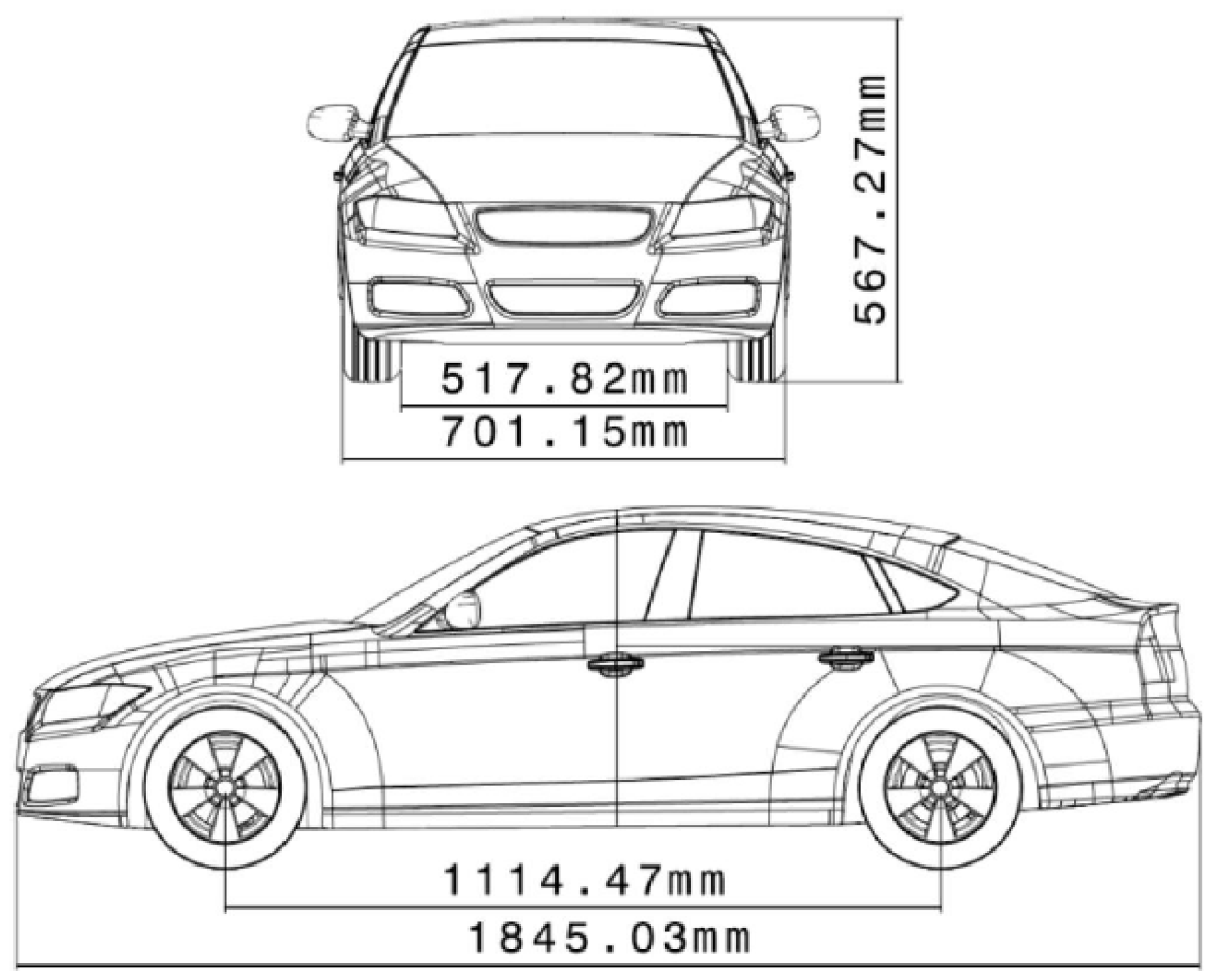
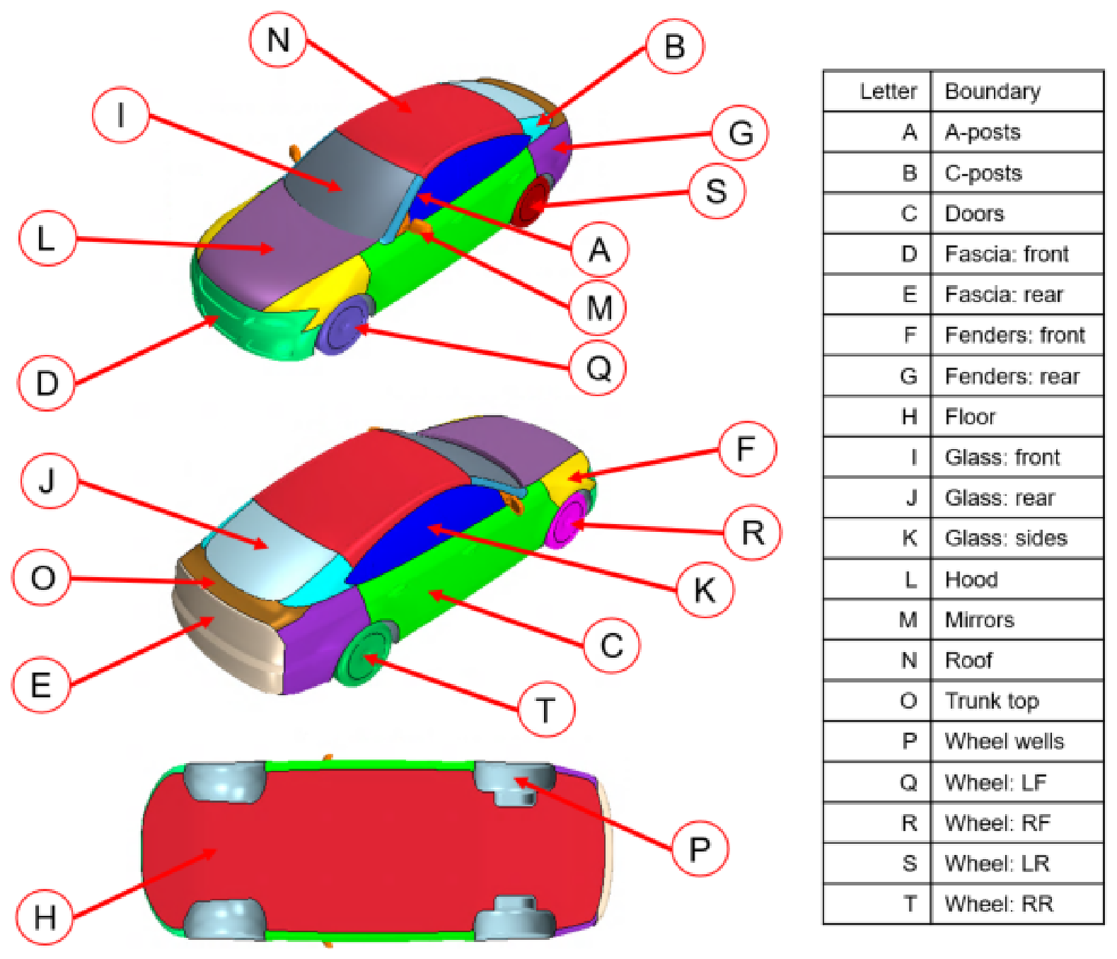
For the acceleration analysis, a 40% scale version of the DrivAer fastback model was considered. The overall vehicle dimensions and configuration are shown in Figure 1. This geometry provides the model used to evaluate the differences between steady, accelerating, and decelerating inlet-flow conditions at a common reference speed. The main exterior surface and component definitions of the DrivAer fastback model are shown in Figure 2. Please note that, given the specific objectives of this study, the original DrivAer geometry was slightly modified to avoid the complexities associated with cooling airflow and wheel-pumping effects. Specifically, the open front grille and five-spoke wheels were replaced with a closed grille and closed wheel rims.

2.3. Computational Domain and Boundary Conditions

The computational domain was used to represent external flow around the DrivAer fastback model in a controlled numerical environment. The vehicle was kept stationary inside the domain while the inlet velocity was varied in time to generate steady, accelerating, and decelerating longitudinal flow conditions. This allowed the acceleration history to be imposed through the free-stream condition without altering the vehicle geometry or domain layout.

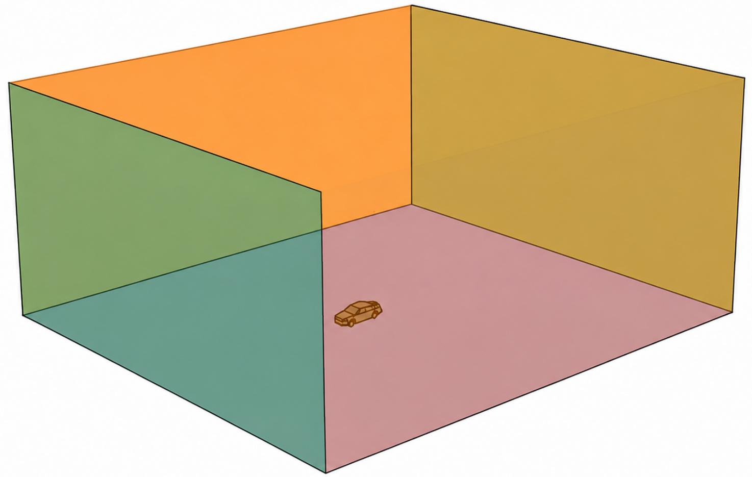
A three-dimensional view of the computational wind-tunnel geometry before the normalized domain dimensions are introduced is provided in Figure 3.

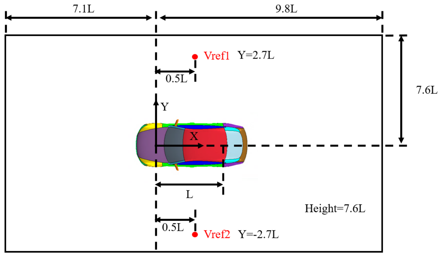
The computational domain layout is shown in Figure 4. The domain dimensions were normalized by the DrivAer wheelbase length, $L=1.114$ m. As shown in the Figure, the inlet side of the domain extends 7.1L upstream of the vertical reference plane, while the downstream side extends 9.8L from this same reference plane. The domain height is shown as 7.6L. This layout provides the numerical space surrounding the vehicle for evaluating the longitudinal acceleration cases.

The Figure also identifies the reference-velocity sampling locations, ${\mathrm{V}}_{\mathrm{ref}1}$ and ${\mathrm{V}}_{\mathrm{ref}2}$, positioned at $Y=2.7L$ and $Y=-2.7L$, respectively. Because the imposed inlet velocity $\left(V\right(t\left)\right)$ varies with time, the flow requires a time-resolved reference velocity. Moreover, owing to blockage and the resulting acceleration of the flow within the simulation domain, the local velocity experienced by the vehicle differs from the prescribed inlet velocity. We, therefore, consider the local measurements to provide a more representative reference for calculating the instantaneous aerodynamic coefficients. Although the vehicle and computational domain are nominally symmetric, this symmetry applies primarily to the time-averaged flow. The instantaneous flow is inherently unsteady and may exhibit asymmetric turbulent fluctuations; consequently, the velocities measured simultaneously at (${\mathrm{V}}_{\mathrm{ref}1}$ and ${\mathrm{V}}_{\mathrm{ref}2}$) may differ. The two locations are, therefore, not used as separate reference velocities. Instead, their instantaneous average is used as a single common reference velocity, reducing sensitivity to local fluctuations and avoiding a bias toward either side of the vehicle.

The motion of the ground and wheel boundaries was defined from the instantaneous reference velocity, $V_{\mathrm{ref}}$. The ground plane was prescribed to translate at $V_{\mathrm{ref}}$, preserving the appropriate relative motion between the vehicle and roadway. Wheel rotation was similarly tied to $V_{\mathrm{ref}}$ through the corresponding angular velocity. Thus, the road and wheel boundary conditions remained kinematically consistent as the vehicle passed through the acceleration and deceleration portions of the cycle.

The velocity inlet is the key boundary condition for the longitudinal acceleration and deceleration cases. The inlet boundary was specified as a velocity inlet, allowing the free-stream velocity to be prescribed as a function of time, $V_{\mathrm{inlet}}\left(t\right)$. For the unsteady DrivAer inlet-velocity signal, the velocity ranged from 25 m s⁻¹ to 55 m s⁻¹, centered around the reference velocity of 40 m s⁻¹. This resulted in a Reynolds number range of $1.78\times {10}^6$ to $3.92\times {10}^6$, based on the DrivAer wheelbase. The inlet turbulence was specified using a non-dimensional turbulence intensity of 0.01 and a synthetic-eddy length scale (see [37]) of 40 mm. As discussed in the Introduction section, the turbulence characteristics of the incoming free stream, including turbulence intensity and length scale, can significantly influence vehicle aerodynamics by affecting boundary-layer development, flow separation, and wake structures. The relatively low free-stream turbulence level prescribed in the present simulations represents a controlled, low-turbulence wind-tunnel environment and was selected to isolate the aerodynamic effects of acceleration and deceleration. However, it is lower than the turbulence levels typically encountered under real-world driving conditions; therefore, the quantitative findings may vary in more turbulent on-road environments. Investigating the combined effects of transient approach-flow velocity and realistic atmospheric or traffic-induced turbulence remains an important direction for future work.

Note that the accelerating and decelerating cases were later compared with the non-accelerating case at the common reference velocity of $V_{\mathrm{ref}}=40$ m s⁻¹.

2.4. Numerical Grid and Mesh Strategy

The computational domain was meshed using an unstructured finite-volume grid with several levels of refinement surrounding the DrivAer fastback. The mesh was designed to provide higher spatial resolution in the near-body and wake regions while avoiding unnecessary refinement in areas where the flow changes more gradually. Smaller cells were, therefore, concentrated around the vehicle surfaces, underbody, wheels, and wake, where larger velocity gradients, boundary-layer development, and separated flow structures are expected, while coarser cells were used farther from the body.

To satisfy the resolution requirements of the IDDES approach, the near-body mesh was guided by the Taylor microscale, $\lambda$, following the recommendation of Kuczaj et al. [38]. The Taylor microscale was taken as a representative turbulent length scale based on Tennekes and Lumley [39]. Surface mesh spacing was selected to remain below this scale, while the wake-region spacing was allowed to increase to approximately twice the Taylor microscale. This distribution places the finest resolution near the body and adjacent shear layers, where smaller turbulent structures are expected, and permits a gradual increase in cell size farther into the wake. Following the approach used by Peters and Uddin [27], the Taylor microscale, $\lambda$, was estimated using the relation given by Tennekes and Lumley [39], as shown in Equation (21):

$$\lambda =\sqrt{15}{\displaystyle \frac{1}{\sqrt{A_1}}}{\displaystyle \frac{1}{\sqrt{Re}}}L,$$

(21)

where $A_1$ is an empirical constant taken as 0.5, $Re$ is the Reynolds number, and L is the characteristic length scale. The resulting Taylor microscale was then used to establish the grid resolution needed to capture the larger inertial-range turbulent structures. As noted by Wilcox [40], the Taylor microscale is approximately 70 times larger than the Kolmogorov length scale. Therefore, the IDDES mesh was intended to resolve the larger turbulent structures while modeling the smaller anisotropic eddies.

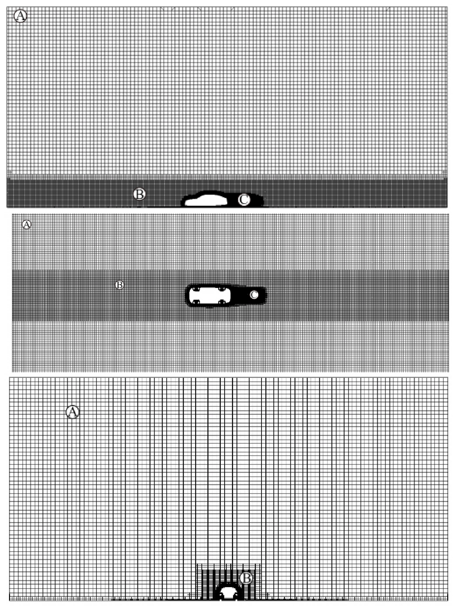
Following this mesh-resolution approach, the computational grid was divided into characteristic refinement regions labeled A through F. The spacing within each region was defined relative to the DrivAer wheelbase length, $L=1.114$ m. The corresponding non-dimensional and dimensional grid-spacing values are provided in

Table 1. DrivAer grid-spacing values non-dimensionalized by wheelbase length, $L=1.114$ m, and exact grid-spacing values.

Mesh Region	A	B	C	D	E	F
Grid Spacing/L	0.144	0.036	0.009	0.0045	0.0023	0.0011
Grid Spacing (mm)	160	40	10	5	2.5	1.25

. These refinement levels produced a gradual transition from the coarser cells in the far field to the finer cells located near the vehicle and within the wake.

The near-body mesh arrangement for refinement regions A, B, and C is shown in Figure 5. These views illustrate the progressive reduction in cell size from the outer portions of the computational domain toward the DrivAer body and adjacent wake region.

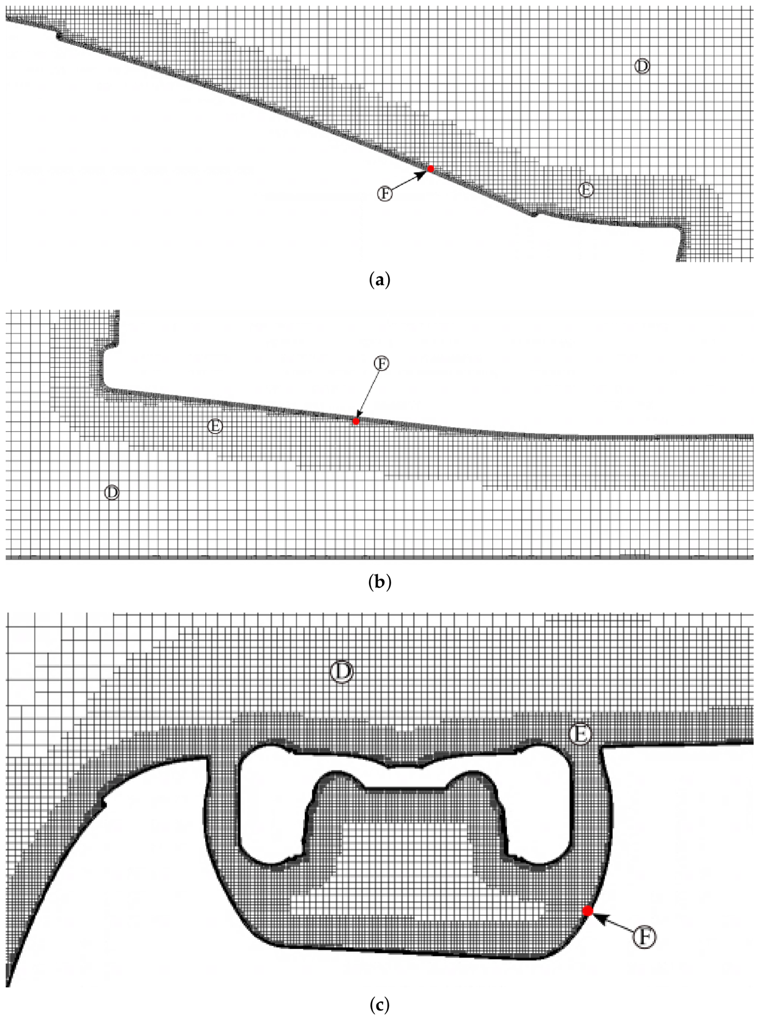
The mesh refinement was arranged progressively from the outer computational domain toward the vehicle. Region A contained the coarsest cells and represented the far-field portion of the grid. Region B used a spacing of 40 mm, corresponding to the synthetic-eddy length scale specified for the inlet turbulence. The grid was further refined through Regions C and D as it approached the vehicle and wake. Region E used a 2.5 mm spacing near the body, corresponding to the calculated Taylor microscale used to guide the near-body refinement, while Region F contained the finest local grid spacing. This progressive refinement provides increased resolution in the near-body and wake regions, where stronger velocity gradients, boundary-layer development, and separated-flow structures are present.

The local mesh distribution is shown in greater detail in Figure 6. The selected views include the rear-glass and decklid region, the front-fascia and underbody region, and the front-wheel region. Additional refinement was applied in these areas because of the local geometric features and flow structures that influence drag, lift, and wake development.

Four wall-normal prism layers were applied along the vehicle surfaces, with a first-layer thickness of 0.5 mm and a total prism-layer thickness of 2 mm. The completed DrivAer mesh contained approximately 42 million unstructured finite-volume cells. This mesh configuration provided the finer spatial resolution required near the vehicle and in separated wake regions while maintaining a practical overall computational cost for the IDDES simulations.

2.5. Physics Models and Solver Settings

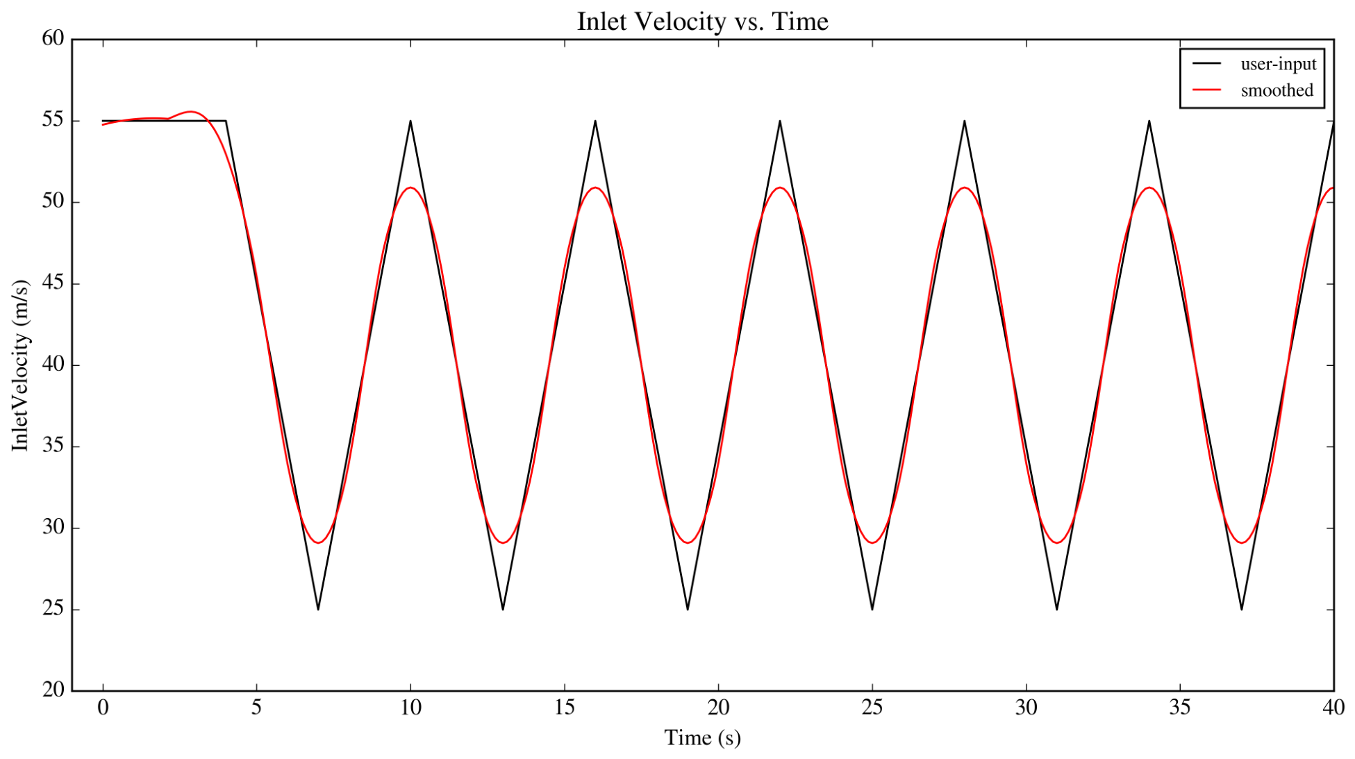
The domain inlet velocity was controlled through a field function that linearly interpolated a file table containing the periodic signal, which was created via a short Python (version 3.6) code allowing the specification of acceleration rate and the min/max velocity; see Figure 7. These inputs were then concatenated together for many periods and then smoothed with the Savitzky–Golay filter [41,42] provided within the Python signal library. Smoothing of the inlet signal was implemented to increase the validity of the simulation results between 35 m s⁻¹ and 45 m s⁻¹ by reducing instantaneous changes in inlet acceleration. With the implementation of a synthetic-eddy-method [37] at the inlet, the inlet turbulence was specified as a non-dimensional turbulence intensity of 0.01 and a synthetic eddy length scale of 40 mm. The inlet velocity was held to 55 m s⁻¹ for 2 s of simulated time before beginning acceleration periods.

STAR-CCM+ v12.02, an unstructured finite volume commercial code, was used to carry out Improved Delayed Detached Eddy Simulations (IDDES) with an unsteady inlet condition to mimic longitudinal acceleration. Velocities ranged from 25 m s⁻¹ to 55 m s⁻¹, resulting in a Reynolds number range (based on wheelbase length L = 1.114 m) from $1.78\times {10}^6$ to $3.92\times {10}^6$, centered around the target velocity of 40 m s⁻¹ and a Reynolds number of $2.85\times {10}^6$. The frontal reference area (including wheels) $A_{\mathrm{ref}}$ = 0.3457 m² was used to calculate force coefficients along with $V_{\mathrm{ref}}\left(t\right)$. When the inlet velocity was equal to 40 m s⁻¹, the timestep was set to 0.0001 s and was increased or decreased with respect to the inlet velocity. This was done to maintain a constant Courant–Friedrichs–Lewy (CFL) value throughout the entire simulated time. Simulations were carried out with constant density air, neglecting compressibility due to the largest free stream mach number being equal to 0.16. The Reynolds Averaged Navier–Stokes (RANS) and Large-Eddy-Simulation (LES) regions utilized bounded central differencing/coupled hybrid second-order upwind spatial schemes, respectively, with a first-order implicit unsteady temporal solver. During each time step, one inner iteration was used primarily to facilitate simulation throughput and save computational resources; this was also implemented during the model validation phase, which concluded that overall body forces were within good agreement with experiments. The Shear Stress Transport (SST) $k-\omega$ DES turbulence model was used with the IDDES transfer function to determine the LES and RANS regions. A total of 6 acceleration–deceleration periods were computed on 144 × 2.4 GHZ Intel Xeon E5-2665 processors in 838.5 h; this implies a total of 120,744 CPU Core-Hours).

3. CFD Process Validation

The DrivAer fastback setup was validated before being used for the acceleration and deceleration analysis. The purpose of the validation step was to confirm that the numerical setup could reasonably reproduce the baseline aerodynamic behavior of the DrivAer fastback model under steady-flow conditions. This is important because the acceleration analysis depends on comparing changes in drag, lift, and wake behavior relative to a reliable baseline vehicle response. The validation was performed using the same underlying setup as the acceleration cases, but with a constant inlet velocity of 40 m s⁻¹ and a constant time step of $1.0\times {10}^{-4}$ s. Forces were averaged between 1 s and 4 s of simulated time. Validation was based on both integrated force coefficients and surface pressure-coefficient distributions along the vehicle centerline.

The integrated force-coefficient comparison is summarized in

Table 2. Force coefficient results from validating the DrivAer fastback model against experiments compiled by Collin et al. [43].

Coefficient	Current CFD	Restraint Corrected	TUM	Audi
$C_D$	0.237	0.244	0.252	0.251
$C_{D,\mathrm{Body}}$	0.186	0.195	0.189	0.196
$C_{D,\mathrm{Wheels}}$	0.051	0.049	0.063	0.055
$C_L$	−0.078	−0.066	–	–
$C_{L,F}$	−0.121	−0.115	–	–
$C_{L,R}$	0.043	0.049	–	–
$C_{L,\mathrm{Body}}$	−0.047	−0.035	−0.008	0.024
$C_{L,F,\mathrm{Body}}$	−0.107	−0.101	−0.063	0.039
$C_{L,R,\mathrm{Body}}$	0.060	0.066	0.055	0.063
$C_{L,\mathrm{Wheels}}$	−0.031	−0.031	–	–

, which includes the experimental data, reported by Collin et al. [43], from two wind tunnels: the Technical University of Munich wind tunnel, identified as TUM, and the Audi Wind Tunnel in Ingolstadt, Germany, identified as Audi. The two facilities employed different wind-tunnel configurations and test conditions, providing a useful basis for evaluating the robustness of the numerical predictions. A comprehensive description of the wind tunnels, floor simulation, wheel-rotation treatment, turbulence conditions, measurement procedures, and applied corrections is provided by Collin et al. [43]. Readers are referred to that study for the complete experimental methodology and associated uncertainties.

Because the vehicle model was restrained differently in the CFD simulations and the wind-tunnel experiments, direct comparison requires correction for support-system effects; further details are provided in the dissertation of Peters [29]. As such, Table 2 also presents restraints-effect-corrected experimental force coefficients, as reported by Collin et al. [43]. The total drag coefficient was underpredicted within approximately 4%, while the body-rear-lift coefficient showed good agreement with the experimental values. The body-front-lift coefficient showed larger variation, which is consistent with the sensitivity of lift measurements to wind-tunnel configuration, restraint effects, wheel modeling, and near-ground flow details. Although there are some discrepancies between the CFD and experimental data, these results were deemed sufficient for carrying out the acceleration study.

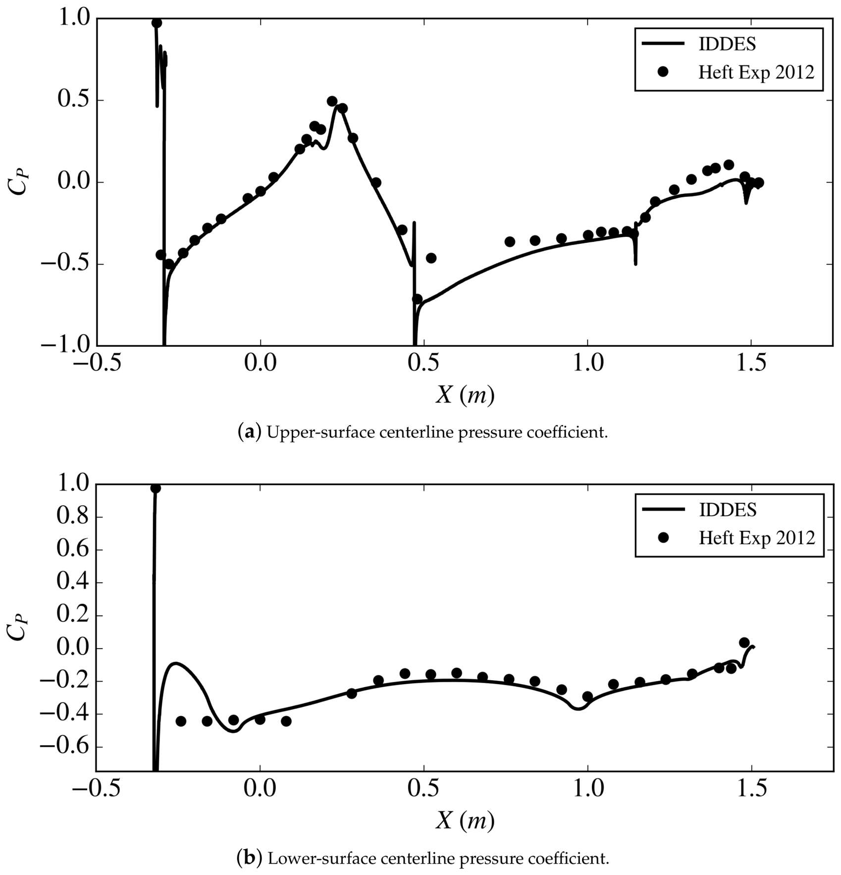
The surface pressure-coefficient comparison was evaluated along the vehicle centerline on the upper and lower surfaces of the model. These comparisons are useful because they show whether the numerical setup captures the main pressure behavior over the hood, roof, rear-glass, decklid, and underbody regions. The upper-surface pressure-coefficient comparison is presented in Figure 8a. This comparison evaluates the IDDES pressure-coefficient prediction against the experimental measurements along the centerline of the upper vehicle surface. Agreement in this region is important because the upper-surface pressure distribution contributes to the rear-body separation, lift behavior, and wake development behind the vehicle. The lower-surface pressure-coefficient comparison is presented in Figure 8b. This comparison evaluates the pressure-coefficient behavior along the lower centerline of the vehicle. The underbody pressure distribution is important because it contributes to the lift and lift-balance behavior that is later evaluated under accelerating, steady, and decelerating inlet-flow conditions.

As a final note, although the pressure-coefficient comparisons showed reasonable overall agreement, several localized discrepancies were observed, including underprediction over part of the roof, reduced positive pressure near the trunk, and a lower-surface difference near the front of the vehicle. These differences were not the primary focus of the validation study, and the baseline model was, nevertheless, considered sufficiently accurate for the acceleration analysis. Taken together, the force- and pressure-coefficient comparisons provide confidence that the baseline DrivAer fastback flow field is represented with adequate fidelity, allowing differences among accelerating, non-accelerating, and decelerating cases to be interpreted primarily as effects of acceleration history rather than as artifacts of numerical or baseline-model error.

4. Data Processing

In the earlier work of Peters and Uddin [27] on the acceleration aerodynamics of flow over a cylinder, the forces from repeated cycles were ensemble-averaged to distinguish the acceleration and deceleration responses. Although effective, this approach requires a relatively long time history containing multiple input cycles. Because the DrivAer simulations are approximately an order of magnitude larger and substantially more computationally expensive, the present study investigates whether second-order least-squares polynomial fits to the acceleration and deceleration force histories can be used to estimate the inertial coefficients from fewer input cycles.

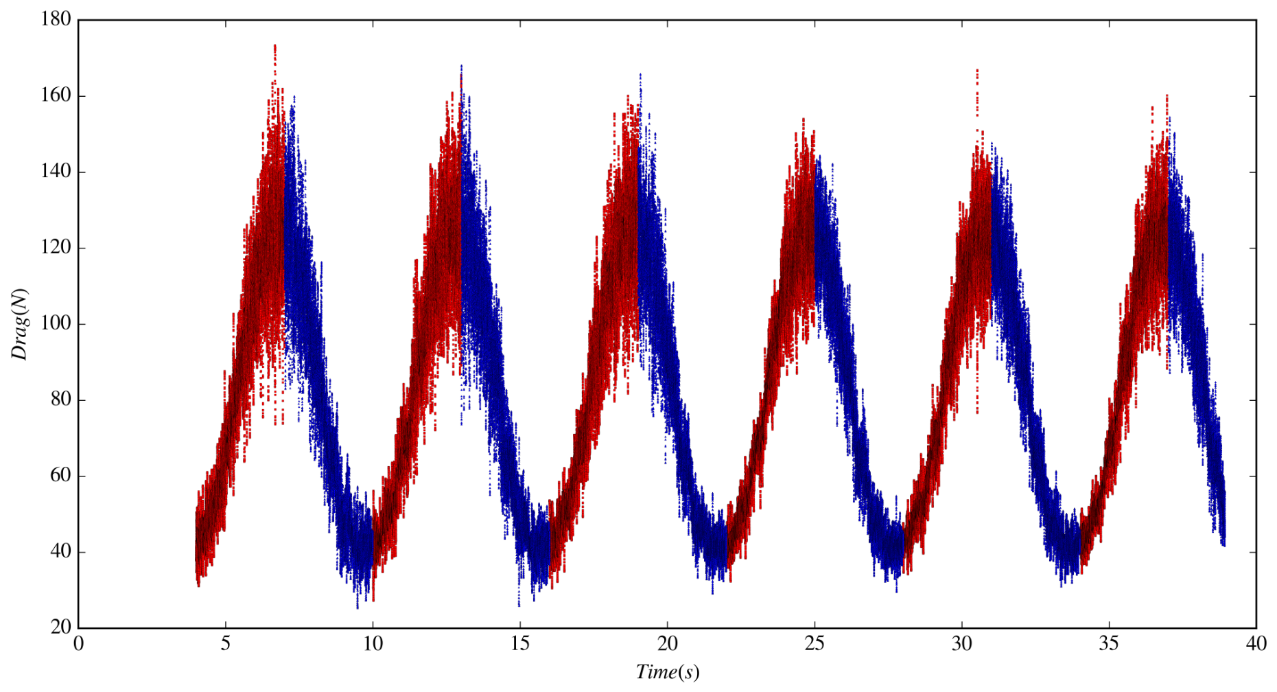
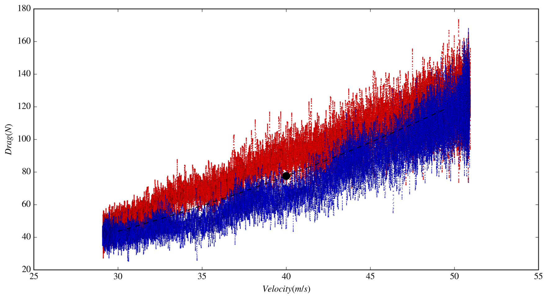
Figure 9 shows the instantaneous drag force on the DrivAer model during acceleration, shown in red, and deceleration, shown in blue, as a function of time. The time histories contain substantial high-frequency fluctuations, making systematic differences between the two conditions difficult to identify directly. These trends are more readily examined by plotting the drag force against the instantaneous reference velocity, $V_{\mathrm{ref}}\left(t\right)$, as shown in Figure 10.

Note that in Figure 10 all six periods are present and the clear trend begins to be apparent: during acceleration (red) the drag force is greater than during deceleration (blue). In addition, the non-accelerating force is plotted at $V_{\mathrm{ref}}=40$ m s⁻¹ as the black dot and is extrapolated over the measured velocity range via the drag force coefficient, which is represented as the dashed black line. The three cases (accelerating, non-accelerating and decelerating) are only equivalent due to noise in the drag force and when the acceleration rates are significantly lower outside of $V_{\mathrm{ref}}=40\pm 7$ m s⁻¹. Further processing is required to determine a quantifiable trend.

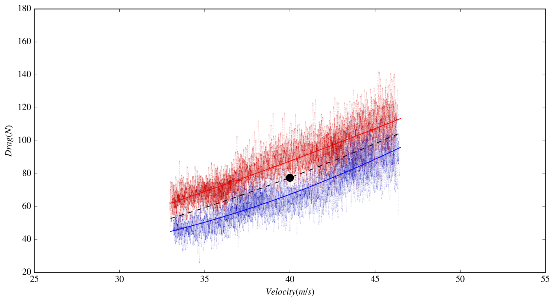
Before fitting a second-order least-squares polynomial to the drag force, data outside the range $V_{\mathrm{ref}}=40\pm 7$ m s⁻¹ were removed to reduce the influence of changing acceleration rates outside the region of interest. Second-order polynomials were then fitted to the accelerating and decelerating drag data, respectively, and can be seen in Figure 11 as the solid red (accelerating) and blue (decelerating) lines where the clear trend is now present between the three cases.

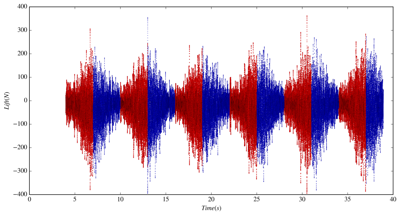
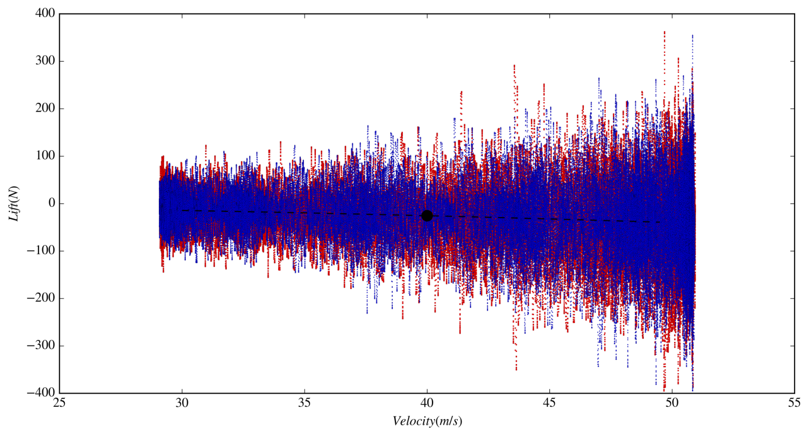
For analyzing lift force, the same process was applied to the time varying lift force seen in Figure 12 where the lift force is noisier in comparison to the drag force. Even when the lift is plotted versus velocity in Figure 13, a discernible trend is not visible.

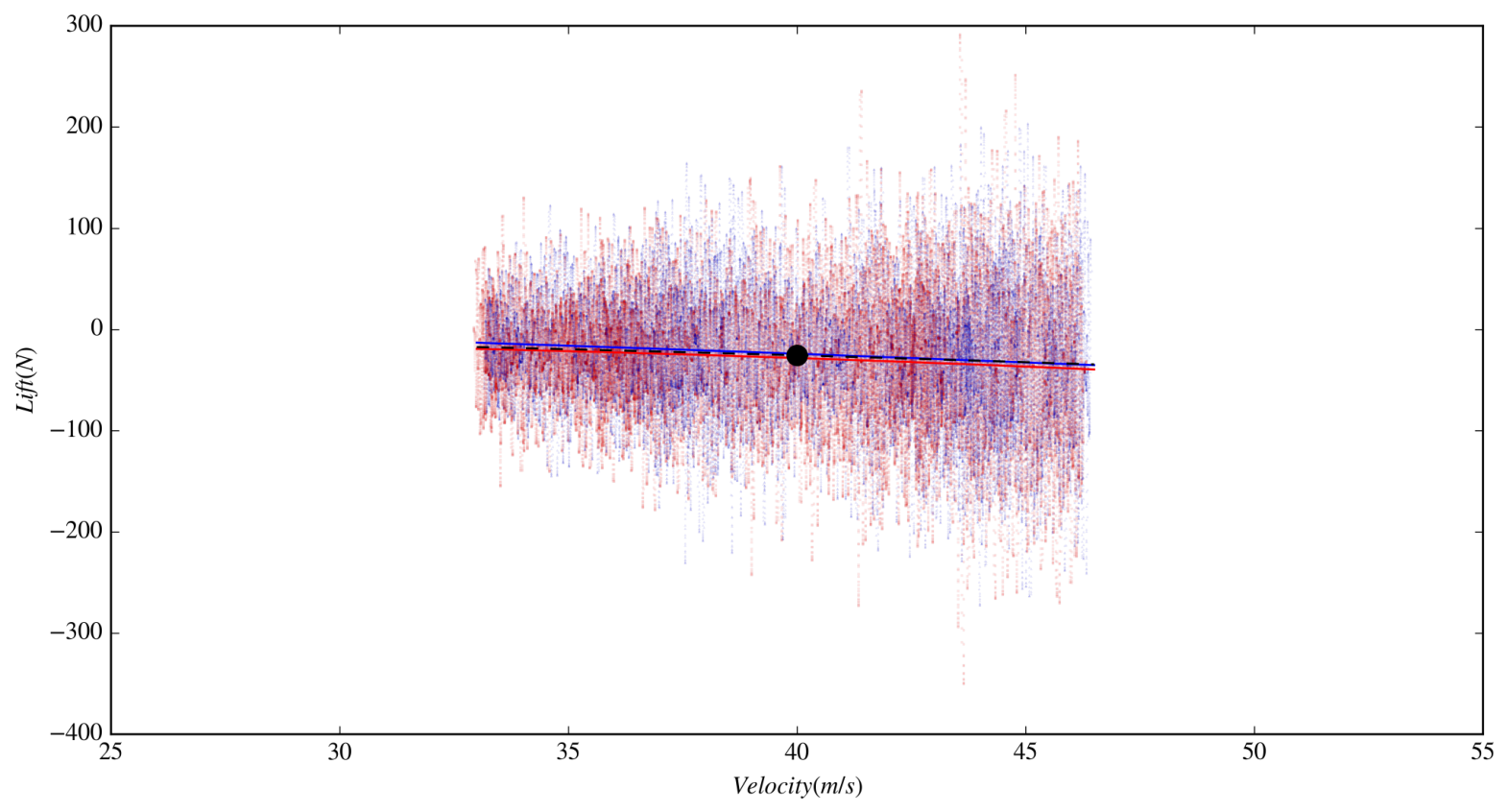
The trend in lift force is not present until a least-squares second order polynomial is fit in Figure 14 and, in comparison to the noise of the lift signal, it is small, but still measurable.

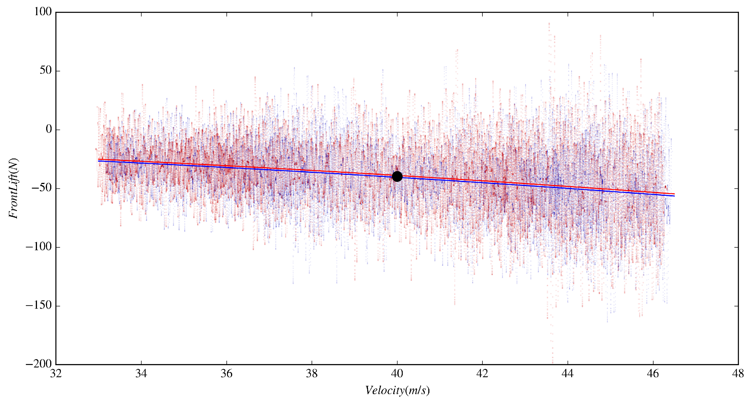
To obtain the front-lift percentage, the same data analysis method was applied to obtain the variation in front lift between the accelerating and decelerating cases, the result of which is presented in Figure 15.

5. Results and Discussion

The overall aerodynamic forces and corresponding inertial coefficients, $C_M$, are summarized in

Table 3. Ensemble-averaged aerodynamic forces for the DrivAer model at $V_{\mathrm{ref}}=40\mathrm{m}{\mathrm{s}}^{-1}$ under deceleration, non-accelerating, and acceleration conditions corresponding to $a_x=-1.5g$, 0, and $+1.5g$, respectively. Drag values were obtained from second-order least-squares polynomial fits, whereas lift values were taken from the filtered force histories rather than the polynomial fits.

${\mathit{a}}_{\mathit{x}}$	Drag (N)	Lift (N)	%Front	${\mathit{C}}_{\mathit{M},\mathbf{Drag}}$	${\mathit{C}}_{\mathit{M},\mathbf{Lift}}$
$-1.5g$	67.49	−24.03	168	2.02	−0.3
0	77.63	−25.55	155	-	-
$1.5g$	87.68	−28.03	137	2.00	−0.54

. The non-accelerating baseline, corresponding to $a_x=0$, was obtained by time-averaging a separate constant-inlet-velocity simulation over a 2 s interval. The accelerating and decelerating force values were obtained from second-order least-squares polynomial fits to the respective force histories.

Note that in Table 3, acceleration is reported in units of gravitational acceleration, g ($g=9.81\mathrm{m}{\mathrm{s}}^{-2}$), to provide a more intuitive indication of the severity of the prescribed maneuvers. This convention is commonly used in motorsports to describe vehicles acceleration and braking. The authors’ broader goal is to extend this research to stock-car racing, which is a primary focus of the research group. Therefore, expressing acceleration in terms of g provides a more meaningful connection to the intended racing application. For example, accelerations of $+15$ and $-15\mathrm{m}{\mathrm{s}}^{-2}$ correspond to approximately $+1.53g$ and $-1.53g$, respectively, which are rounded to $\pm 1.5g$. These values represent aggressive high-performance driving rather than typical passenger-vehicle operation. All calculations, however, are performed using SI units.

Relative to the non-accelerating baseline, the drag force changed by approximately $\pm 13\%$ under acceleration and deceleration. The nearly symmetric response produced an inertial drag coefficient of approximately $C_M=2$. This behavior differs from that reported for the channel-mounted cylinder studied by Peters and Uddin [27], for which the acceleration and deceleration responses were markedly asymmetric. The difference is likely associated with the substantially greater geometric complexity of the DrivAer model, its proximity to the ground, and the presence of multiple interacting separation regions in the vehicle’s wake.

The lift response also differed fundamentally from that of the isolated cylinder. In the cylinder study, the ensemble-averaged lift remained essentially unchanged because the body was symmetrically positioned within the channel and sufficiently far from surrounding boundaries. The DrivAer model, by contrast, operates in close proximity to the ground and exhibits a nonzero baseline lift distribution, with front-axle downforce and rear-axle lift. In addition, the rear-window and deck geometry promote separation and wake development that may respond differently during acceleration and deceleration. Consequently, the longitudinally accelerating cases produced measurable changes in total lift, indicating that separate inertial lift coefficients are required to characterize the transient aerodynamic response.

Because the baseline net lift was relatively small, even modest absolute changes produced appreciable percentage differences. Relative to the non-accelerating condition, the total lift changed by $-5.9\%$ during deceleration and by $9.7\%$ during acceleration, corresponding to inertial lift coefficients of $-0.30$ and $-0.54$, respectively. The unequal magnitudes of these coefficients indicate that the lift response is not symmetric with respect to the sign of the longitudinal acceleration.

The aerodynamic balance, or “%Front”, defined as the ratio of the front lift to total lift, was also strongly affected. During the validation study, the front-lift percentage exceeded $100\%$, reaching approximately $155\%$, because the vehicle generated downforce at the front axle while simultaneously producing lift at the rear axle. Under acceleration, the front-axle downforce was reduced while the overall vehicle downforce increased, indicating a rearward shift in aerodynamic balance. This interpretation is consistent with the corresponding change in front-lift percentage, which decreased by approximately 18 percentage points during acceleration relative to the non-accelerating condition and increased by approximately 13 percentage points during deceleration. These results demonstrate that longitudinal acceleration affects not only the total aerodynamic loads but also their axle-wise distribution, with direct implications for transient vehicle stability, tire loading, and control-system performance.

To complement the force- and balance-based analysis presented above, the corresponding ensemble-averaged flow fields were examined to identify the aerodynamic mechanisms underlying the observed differences between acceleration and deceleration. The ensemble-averaged fields retain some spatial variability because the finite number of acceleration cycles does not fully suppress the broadband fluctuations associated with shear-layer dynamics, boundary-layer development, and wake unsteadiness. Nevertheless, the averaging procedure is sufficient to reveal several coherent and physically consistent differences between the accelerating and decelerating conditions. These trends provide useful insight into the transient aerodynamic response of the DrivAer model, while additional cycles in future studies would further improve statistical convergence and sharpen the spatial definition of the observed structures.

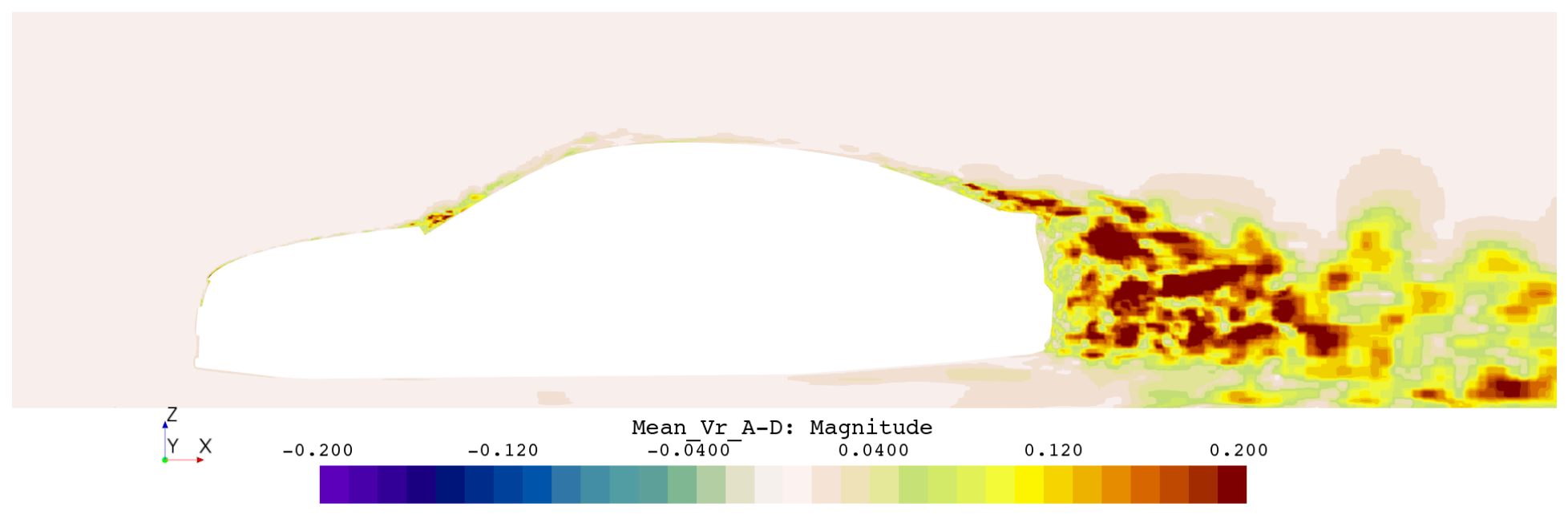
The velocity magnitude was normalized by the instantaneous reference velocity, $V_{\mathrm{ref}}$, and is denoted by $V_r$. Figure 16 presents the centerline difference in normalized velocity, $\Delta V_r=V_{r,\mathrm{acc}}-V_{r,\mathrm{dec}}$, at $Y=0$. Several distinct features are evident:

• Near the base of the windshield, $\Delta V_r$ is positive, indicating that the accelerating case produces a locally higher normalized velocity by approximately $0.2$. A similar trend was observed in the earlier cylinder study, although the cylinder exhibited larger wake differences.
• Over the upper surface of the rear decklid, the accelerating case exhibits higher normalized velocity than the decelerating case. This behavior is consistent with reduced separation over the rear glass during acceleration and enhanced separation during deceleration.
• The accelerating case also produces higher normalized velocity in the near wake, whereas the decelerating case exhibits a larger velocity deficit. This result further indicates that acceleration history modifies the strength and structure of the separated wake.

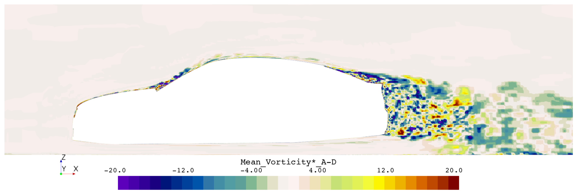
To further interpret the velocity-field differences discussed above, the vorticity magnitude was non-dimensionalized using the characteristic time scale $L/V_{\mathrm{ref}}\left(t\right)$ and is denoted by ${\omega }^{*}$. Figure 17 presents the centerline difference, $\Delta {\omega }^{*}={\omega }_{\mathrm{acc}}^{*}-{\omega }_{\mathrm{dec}}^{*}$, at $Y=0$. Despite the residual spatial variability in the ensemble-averaged field, several coherent trends are evident:

• A localized increase in ${\omega }^{*}$ occurs near the leading edge of the hood, indicating stronger vorticity generation in this region during acceleration.
• Along much of the upper vehicle surface, $\Delta {\omega }^{*}$ is negative near the wall, indicating greater near-wall vorticity during deceleration. A similar behavior was observed in the earlier cylinder study.
• Reduced vorticity is observed over the rear glass and trunk during acceleration. This feature is consistent with an acceleration-dependent shift in the rear-glass separation and the associated shear-layer trajectory. An analogous displacement of the separated shear layer was also identified in the cylinder study.
• The vehicle wake exhibits predominantly negative $\Delta {\omega }^{*}$, indicating stronger wake vorticity during deceleration. This trend is consistent with both the larger velocity deficit identified in the decelerating case and the corresponding observations from the cylinder investigation.

Taken together, the velocity- and vorticity-difference fields show that longitudinal acceleration alters not only the magnitude of the aerodynamic forces but also the development, position, and strength of the vehicle shear layers and wake. The recurrence of several trends previously observed for the channel-mounted cylinder suggests that these effects are not unique to a particular geometry, while the additional features associated with the ground plane, rear-glass separation, and vehicle-specific wake topology demonstrate the greater complexity of the road-vehicle response.

6. Conclusions

This study addressed the fundamental question of whether acceleration aerodynamics is significant for road vehicles. Although broad in scope, this question represents an essential first step in determining whether the associated physical effects justify further investment of experimental and computational resources. Answering it required the development of a new numerical framework and analysis strategy based on IDDES simulations, drawing on concepts and methods established across the prior literature. The framework developed here builds on the earlier platform introduced by Peters and Uddin [27], which employed a channel-mounted bluff body that could be validated against an extensive body of experimental and numerical data before the methodology was extended to a realistic road-vehicle geometry. In the present work, the DrivAer fastback model was subjected to longitudinal acceleration and deceleration using the same time-varying inlet-velocity approach. By comparing decelerating, constant-speed, and accelerating conditions at $V_{\mathrm{ref}}=40\mathrm{m}{\mathrm{s}}^{-1}$, the analysis distinguished acceleration-history effects from changes attributable solely to instantaneous flow speed. The principal conclusions of the study are summarized below.

The integrated force results showed that the DrivAer fastback does not produce the same aerodynamic loading when the acceleration state is different. Relative to the non-accelerating case, drag decreased by approximately 13.1% during deceleration and increased by approximately 12.9% during acceleration. The lift force also changed, with acceleration producing a more negative lift value and deceleration producing a less negative lift value. In addition, the % Front value changed from 155 in the non-accelerating case to 168 during deceleration and 137 during acceleration, indicating a shift in the front-to-rear distribution of aerodynamic loading.

The flow-field comparisons further support these force trends. Differences in non-dimensional velocity and vorticity magnitude were observed near the rear-glass, decklid, and wake regions, indicating that the rear-body flow structure changes between accelerating and decelerating conditions. These wake-field differences suggest that the acceleration-history effect is connected to changes in separated flow behavior, rather than only changes in the integrated force values.

Overall, the results demonstrate that a quasi-steady interpretation based solely on instantaneous velocity is insufficient to characterize the aerodynamic response of the DrivAer fastback under longitudinal acceleration and deceleration. At the same reference velocity, the vehicle exhibits distinct drag, lift, aerodynamic balance, and wake behavior depending on whether the flow is accelerating or decelerating, indicating that the aerodynamic response retains a measurable memory of its prior transient evolution. Future work should, therefore, consider additional acceleration profiles and cycles, alternative vehicle configurations, and a more detailed investigation of the wake mechanisms responsible for the observed force differences. The present polynomial-based force analysis should also be complemented by more advanced time-series and modal-analysis methods, particularly dynamic mode decomposition (DMD), which was first introduced by Schmid [44] and subsequently applied to a range of ground-vehicle aerodynamic flows [45,46,47,48], as well as to deep-learning-based surrogate models [49]. These approaches could provide a more complete characterization of the time-dependent behavior of integral aerodynamic quantities, including drag, lift, and aerodynamic moments, while also identifying the dominant coherent flow structures, their temporal evolution, and their direct contribution to the acceleration-dependent loads observed in this study.