Two-Speed AMT Shift Control Strategy Based on Vehicle Speed Prediction and Driving Style Recognition for Heavy-Duty Electric Vehicles

Abstract

The two-speed transmission system significantly enhances the powertrain matching performance of heavy-duty electric military armored vehicles by optimizing high-torque output at low speed and energy efficiency at high speed. However, most existing electric vehicles do not incorporate driving styles or real-time driving condition prediction into their shift control strategies, resulting in suboptimal gear shift timing and smoothness that fail to align with driver expectations and operational requirements. To address these limitations, this study focuses on the two-speed automated manual transmission (AMT) system in heavy-duty electric military armored vehicles. Firstly, a comprehensive shift control model is established, integrating key components such as the drive motor and power battery. Furthermore, a shift control strategy based on vehicle speed prediction and driving style recognition is proposed. The operational logic of this strategy is systematically analyzed under various driving cycles. Simulation and hardware-in-the-loop (HIL) results confirm the performance gains. Simulation and hardware-in-the-loop (HIL) results indicate that the proposed approach improves vehicle power performance by 21.36%, increases energy efficiency by 3.94%, and reduces powertrain shock by 31.81% compared to the conventional vehicle-speed-based gear shifting method. Compared to the adaptive shift schedule design method, the proposed approach reduces shifting frequency by 21.43% and improves ride comfort by at least 19.17% while maintaining comparable dynamic performance and energy efficiency.

1. Introduction

In recent years, the challenges posed by energy scarcity and environmental pollution have grown increasingly severe, prompting a global shift toward energy conservation and emission reduction [1]. Electric vehicles (EVs) have become an effective tool for green travel due to their potential to improve energy efficiency and reduce environmental pollution [2,3]. The shifting performance of electric vehicles is subject to increasingly strict requirements from consumers [4]. The adoption of two-speed transmissions has significantly enhanced powertrain efficiency in heavy-duty EVs by optimizing low-speed torque delivery and high-speed energy efficiency [5,6]. Conventional shift control strategies typically determine shift points based on vehicle speed. A large number of scholars employ advanced algorithms such as model predictive control (MPC) and dynamic programming to enhance shift quality. These approaches have achieved notable progress in addressing key challenges in this domain. For instance, Ivan C et al. developed a static model-based predictive control (S-MPC) strategy, which provided a pre-specified shift time and avoided the chatter effect by using control input blind zone components, thereby relaxing the shift time accuracy to a certain extent [7]. Ranogajec V et al. designed a segmented linear control strategy for the dual-shift downshift process of an automatic transmission through a multi-objective optimization method, and verified that the strategy based on the rapid release and disengagement of the clutch had the optimal comprehensive performance [8]. Kihan K et al. optimized shift control through proxy models, variable transmission ratios, and adaptive transmission modes, which emphasized the importance of accounting for variable transmission efficiency; their approach improved energy efficiency and dynamic performance by 12.1% and 10.7%, respectively, compared to single-speed transmission EVs [9].

Nevertheless, existing methods often fail to consider driving style and real-time prediction of vehicle speed, leading to unsatisfactory shift timing, speed, and frequency that may not align with driver expectations [10]. In recent years, some scholars have considered aspects, such as driving style identification, vehicle speed forecasting, and driving intention analysis, which can effectively enhance gear shifting performance. Xi J et al. proposed a torque control strategy based on driving intention, which can achieve optimization of shift quality [11]. Chen Z et al. developed an online predictive energy management strategy to effectively mitigate the performance degradation caused by inaccurate driving cycle predictions [12]. Kang M et al. formulated an eco-gear shift control strategy by discretizing vehicle speed to construct a Markov chain model and applied a dynamic programming algorithm with algebraic operations to improve vehicle fuel economy [13]. Liu X et al. developed an adaptive shift schedule design method for multi-gear AMT electric vehicles, which significantly enhanced dynamic performance, energy economy, and shift adaptability in varying driving cycles [14].

To further improve vehicle power performance, energy efficiency, and ride smoothness, and to address the issue where the shift timing, speed, and frequency fail to meet the driver’s expectations, this study focuses on the two-speed AMT system in heavy-duty electric military armored vehicles. A comprehensive shift control model incorporating the drive motor, power battery, and transmission dynamics is established. Furthermore, a novel shift control strategy considering both driving style classification and predictive vehicle speed information is proposed. The operational logic of the proposed strategy in various driving cycles is systematically analyzed. The main contributions of this work are summarized as follows:

(1)

A shift control strategy is proposed based on fuzzy control that integrates a driving style recognition model based on impact degree analysis, a Markov chain vehicle speed prediction model, and an adaptive model to avoid frequent shifting. This strategy makes real-time decisions on the gear that best meets the driver’s driving needs by considering the dynamic interaction relationship between the identified driver’s driving style and the real-time predicted future vehicle speed. It effectively compensates for the shortcomings of existing theories that focus on static analysis.

(2)

A fourth-order probability output matrix of the Markov chain model based on the driving condition database was developed to represent the relationship between vehicle speed and acceleration. The vehicle speed prediction model based on this matrix can accurately predict the vehicle speed in the next 2 s based on the current vehicle speed.

(3)

A shift execution strategy for precisely controlling the rotational speed of the shift motor was designed to reduce the impact during shifting. By taking the rotational speed difference of the synchronizer and its rate of change into account, a fuzzy controller is designed to control the shifting speed, thereby effectively reducing the impact of shifting and improving driving smoothness.

The rest of this paper is organized as follows. In Section 2, a two-speed AMT shift control simulation model for electric heavy-duty vehicles is developed based on the MATLAB/Simulink environment (version R2024b). The model incorporates key components such as the drive motor, power battery, and transmission system, laying the foundation for subsequent research. Section 3 establishes a driving style recognition model based on impact degree, a vehicle speed prediction model based on the Markov chain model, an adaptive model to avoid frequent gear shifting, and a gear shifting execution model considering driving intent. Section 4 presents a comparative analysis conducted in the MATLAB/Simulink environment using driving cycles to evaluate the performance of the optimized control model against both the conventional and adaptive methods. Additionally, experimental validation was performed on a HIL testing for the shift motor to verify the feasibility of optimizing the shift execution process through speed regulation. Section 5 concludes the article.

2. System Modeling

In this section, a two-speed AMT shift control simulation model for electric heavy-duty vehicles is developed based on the MATLAB/Simulink environment. The model incorporates key components such as the drive motor, power battery, and transmission system, laying the foundation for subsequent research.

2.1. Drive Motor Modeling

The drive motor has been selected as a permanent magnet synchronous motor for electric two-speed AMT heavy-duty vehicles in this section, featuring high efficiency, high power density, and excellent dynamic response characteristics. Under normal circumstances, the modeling of permanent magnet synchronous motors needs to take into account multiple physical field coupling factors such as core saturation effect, demagnetization characteristics of permanent magnets, and temperature drift. To simplify the analysis, this paper ignores the magnetic saturation effect, core loss, and symmetry of the three-phase windings, and assumes that the magnetic field distribution is a sine wave.

The spatial vector relationship between the stator rotating magnetic field and the constant magnetic field in permanent magnet synchronous motors provides a physical theoretical basis for d-q coordinate transformation. Let the d-axis be the direction of the rotor magnetic field and the q-axis be perpendicular to it. Establish the d-q rotational coordinate system and establish the voltage equation of the motor [15]:

$$u_d=R_s{i}_d+L_d{\displaystyle \frac{d{i}_d}{dt}}-{\omega }_e{L}_q{i}_q$$

(1)

$$u_q=R_s{i}_q+L_q{\displaystyle \frac{d{i}_{\mathrm{q}}}{dt}}-{\omega }_e\left(L_d{i}_d+{\psi }_f\right)$$

(2)

where i_d and i_q are the currents along the d and q axes, respectively. R_s is the stator resistance; L_d and L_q are the inductors of the d and q axes, respectively. ω_e is the electrical angular velocity; ψ_f is the permanent magnet flux link; and u_d and u_q represent the voltages along the d and q axes, respectively.

The electromagnetic torque equation of the permanent magnet synchronous motor is:

$$T_e={\displaystyle \frac{3}{2}}p\left[{\psi }_f{i}_q+\left(L_d-L_q\right)i_d{i}_q\right]$$

(3)

where p is the number of pole pairs on the motor; T_e stands for electromagnetic torque.

The motion equation of the motor is:

$$\begin{array}{c}{T}_e-T_L=I_d{\displaystyle \frac{d{\omega }_m}{dt}}+B{\omega }_m\end{array}$$

(4)

where T_L represents the load torque; I_d is the moment of inertia of the drive motor; B is the damping coefficient; and ω_m represents the mechanical angular velocity.

Based on the existing parameters of the permanent magnet synchronous motor already installed on the electric two-speed AMT heavy-duty vehicle as the research object, a drive motor model is established, and the parameters of the drive motor are as follows.

As shown in

Table 1. Parameters of the drive motor.

Parameter	Value	Units
The maximum rotational speed	8000	r/min
Peak power	230	kW
Rated power	165	kW
Peak torque	1100	N·m

, among the parameters of the drive motor, the maximum speed of the permanent magnet synchronous motor is 8000 r/min, the peak power is 230 kW, the rated power is 165 kW, and the peak torque is 1100 N·m.

2.2. Power Battery Modeling

Power batteries have the function of energy recovery [2]. When braking or coasting, they recover kinetic energy and store it in the battery, further affecting the vehicle’s range [16,17]. Lithium-ion batteries were selected to build a battery model in order to analyze the changes in the state of charge (SOC) under different shift strategies [18]. The electromotive force and internal resistance model of the battery can be obtained through experiments:

$$E_{SOC}=E_0+{\displaystyle \sum _{j=1}^5{E}_{j}SO{C}^j}$$

(5)

$$R_{SOC}={\delta }_0\left(R_0+{\displaystyle \sum _{j=1}^6{\lambda }_{j}SO{C}^j}\right)$$

(6)

where E_SOC represents the electromotive force in the current state. E₀ is the fitting coefficient of the battery electric constant; SOC is the state of charge. R_SOC represents the current internal resistance; δ₀ is the internal resistance compensation coefficient; R₀ is the internal resistance constant; λ_j is the fitting coefficient; and j represents a polynomial exponential degree, which is used to describe the nonlinear relationship between the electromotive force and internal resistance of a battery and its state of charge. According to the fitting accuracy, the quintic polynomial and the sextuple polynomial are taken, respectively. (see Appendix A).

The calculation formula for SOC is as follows [19]:

$$SOC(t+1)=SOC(t)-{\displaystyle \frac{I(t)}{Q_{bat}}}$$

(7)

$$I(t)={\displaystyle \frac{E_{SOC}-\sqrt{E_{SOC}^2-4P_{bat}{R}_{SOC}}}{2R_{SOC}}}$$

(8)

$$\mathrm{\Delta }SOC={\displaystyle \frac{E_{SOC}-\sqrt{E_{SOC}^2-4P_{bat}{R}_{SOC}}}{2R_{SOC}{Q}_{bat}}}$$

(9)

where t represents a discrete time step; I represents the current. As E_SOC and R_SOC are dynamically adjusted with SOC(t), I(t) is indirectly adjusted with t. Q_bat stands for capacitance; P_bat stands for power.

Based on Equations (5)–(9), the battery model was established to build the shift control model and complete the simulation analysis.

2.3. Transmission System Modeling

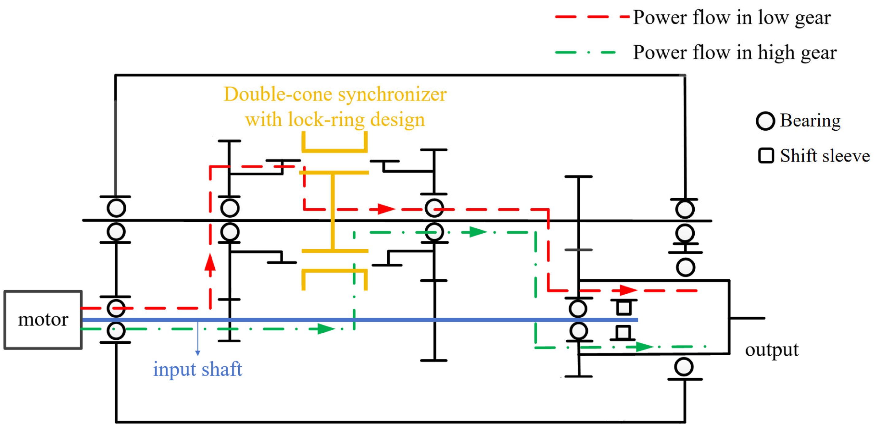
A transmission system model is built to facilitate the calculation of the relationship between the gear speed of the synchronizer and the vehicle speed of the entire vehicle. Its specific parameters are shown in

Table 2. Parameters of the transmission system model.

Parameter	Value	Units
Wheel radius	0.31	m
The transmission ratio of the first gear	2.05	/
The transmission ratio of the second gear	1.03	/
The speed ratio of the main reducer	2.45	/
The reduction ratio of the side reducer	5.05	/

.

In addition to determining the parameters of the transmission system model, when building the transmission system model, a schematic diagram of the transmission system must be designed. The specific transmission principle is shown in Figure 1.

Based on the transmission system model, it is not difficult to calculate the relationship between the gear speed of the synchronizer, the output speed of the drive motor, and the vehicle speed of the entire vehicle:

$$n_0={\displaystyle \frac{n_1}{i_0{i}_1{i}_3}}$$

(10)

v = n₀·2πr

(11)

v = n₁·2πr/(i₀i₁i₃)

(12)

$$n_Q=n_0{i}_Q$$

(13)

where i₁ represents the first gear transmission ratio; i₂ is the second gear transmission ratio. The speed ratio of the main reducer is i₀; i₃ is the reduction ratio of the side reducer; i_Q is the ratio of the drive motor speed to the synchronizer speed at the current gear; r represents the radius of the wheel; n₀ represents the wheel speed; n₁ represents the gear speed of the synchronizer; n_Q represents the output speed of the drive motor; and v represents the vehicle speed.

To conduct the economic simulation analysis, the torque signal and the speed signal of the driving motor were collected. The power of the driving motor was calculated through Equation (14) [20].

$$P={\displaystyle {\int }_0^T\frac{T_e{n}_Q}{9550\times 60\times 60}}dt$$

(14)

where P is the total energy consumption of the driving motor; n_QG is the ratio of the output speed of the drive motor to the speed of the synchronizer gear at the high-speed gear; and n_QD is the ratio of the output speed of the drive motor to the speed of the synchronizer gear at low speed.

2.4. Vehicle Longitudinal Dynamics Modeling

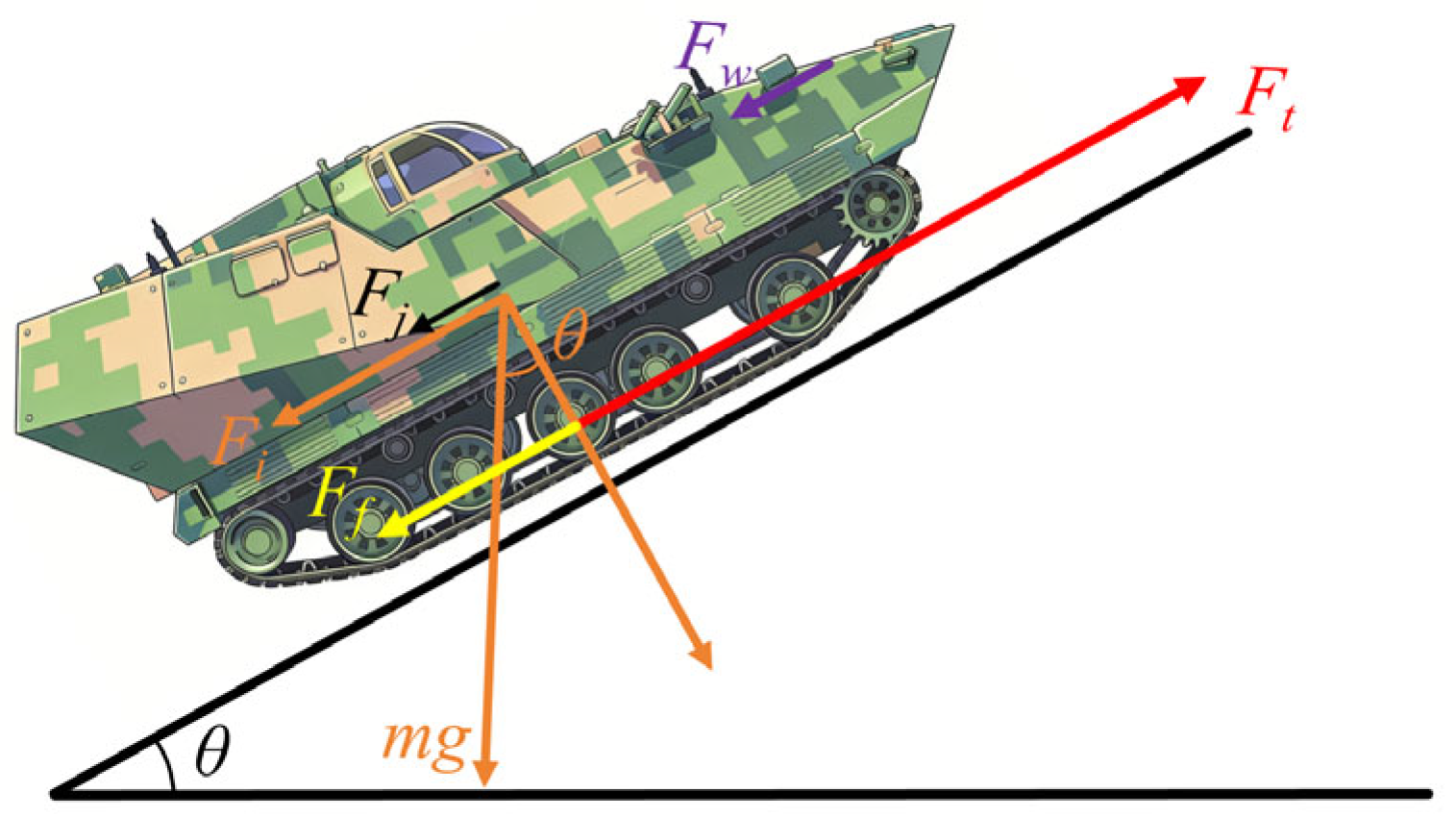
The total mass of the two-speed AMT heavy electric military vehicle is 15,000 kg. The longitudinal force is shown in Figure 2, and the vehicle’s driving state is as follows:

F_t = F_f + F_w + F_j + F_i

(15)

where F_t represents the driving force of the entire vehicle; F_f is the rolling resistance; F_w stands for air resistance; F_j is the acceleration resistance; and F_i is the slope resistance.

The driving force is transmitted from the torque output by the motor to the wheels through the transmission and the drive shaft:

$$F_t={\displaystyle \frac{T_e·i·\eta }{r}}$$

(16)

where i is the current gear transmission ratio; η is the efficiency of the transmission system; r represents the radius of the wheel; and T_e represents the output torque of the drive motor.

The rolling resistance is as follows:

$$F_f=C_{f}mg\cos \theta$$

(17)

where C_f is the rolling resistance coefficient; θ is the slope angle.

The air resistance is as follows:

$$F_w={\displaystyle \frac{1}{2}}\rho C_{d}A{v}^2$$

(18)

where ρ represents the density of air; C_d is the coefficient of air resistance; and A represents the windward area of the vehicle.

The acceleration resistance is as follows:

$$F_j=\delta m{\displaystyle \frac{dv}{dt}}$$

(19)

where δ represents the rotational mass conversion factor.

The resistance of the ramp is as follows:

$$F_i=mg\sin \theta$$

(20)

From this, it is not difficult to obtain that the driving equation for electric vehicles is:

$${\displaystyle \frac{T_{e}i\eta }{r}}=C_{f}mg\cos \theta +{\displaystyle \frac{1}{2}}\rho C_{d}A{v}^2+\delta m{\displaystyle \frac{dv}{dt}}+mg\sin \theta$$

(21)

3. Main Results

This section establishes a driving style recognition model based on impact degree, a vehicle speed prediction model based on the Markov chain model, an adaptive model to avoid frequent gear shifting, and a gear shifting execution model considering driving intent.

3.1. Shift Decision System Design

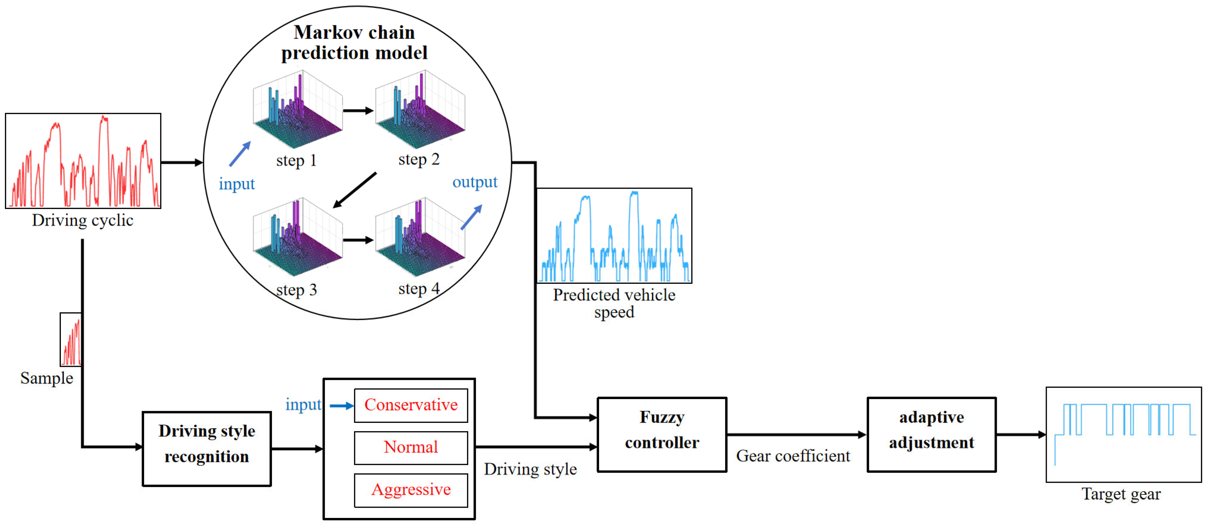
The designed fuzzy PID shift control strategy is based on driving style and vehicle speed prediction, which aims to optimize the shift strategy according to factors such as the driver’s driving habits, vehicle performance, and road conditions, and hence to achieve a more efficient and comfortable driving experience. To formulate the fuzzy PID electric vehicle shift control strategy based on driving style and vehicle speed prediction, the scheme shown in Figure 3 was developed.

To optimize the shift decision-making process, it is necessary to predict the changes in vehicle speed. As shown in the scheme in Figure 3, a Markov chain prediction model was constructed to predict the road conditions in real time. Under the premise of collecting vehicle speed and vehicle acceleration signals, through a large amount of data comparison, an iterative prediction method is adopted to predict the vehicle speed changes 2 s later relatively accurately, obtaining the predicted road conditions. To formulate corresponding shift rules according to different driving styles [21], historical vehicle speeds within a 120 s driving period are sampled, and the degree of change in vehicle acceleration (shock degree) within the sampling period is analyzed. Finally, the driving style recognition model is used to judge the shock degree of the vehicle, identifying the different driving styles of the driver. Based on the obtained predicted road conditions and driving styles, a fuzzy controller is built with the predicted road conditions and driving styles as inputs and the gear coefficient as the output. The gear coefficient output by the fuzzy controller is adaptively adjusted to obtain the target gear for the shift strategy.

3.2. Driving Style Recognition Model Based on Impact Degree

When different drivers operate vehicles, they often have different driving styles [22,23,24]. To adapt to drivers of different styles, it is necessary to identify the driving styles to meet different driving needs [25]. In electric vehicles, the driver’s usage habits of the accelerator pedal can be fed back by the rate of change in the torque of the drive motor. Equation (22) presents the relationship formula of the torque change rate of the driving motor [26]:

$${\dot{T}}_e={\displaystyle \frac{d{T}_e}{dt}}={\displaystyle \frac{i_0(I_{out}+i_g^2{T}_e)}{i_{g}r}}$$

(22)

where i_g represents the AMT transmission ratio; I_out represents the moment of inertia of the AMT output shaft.

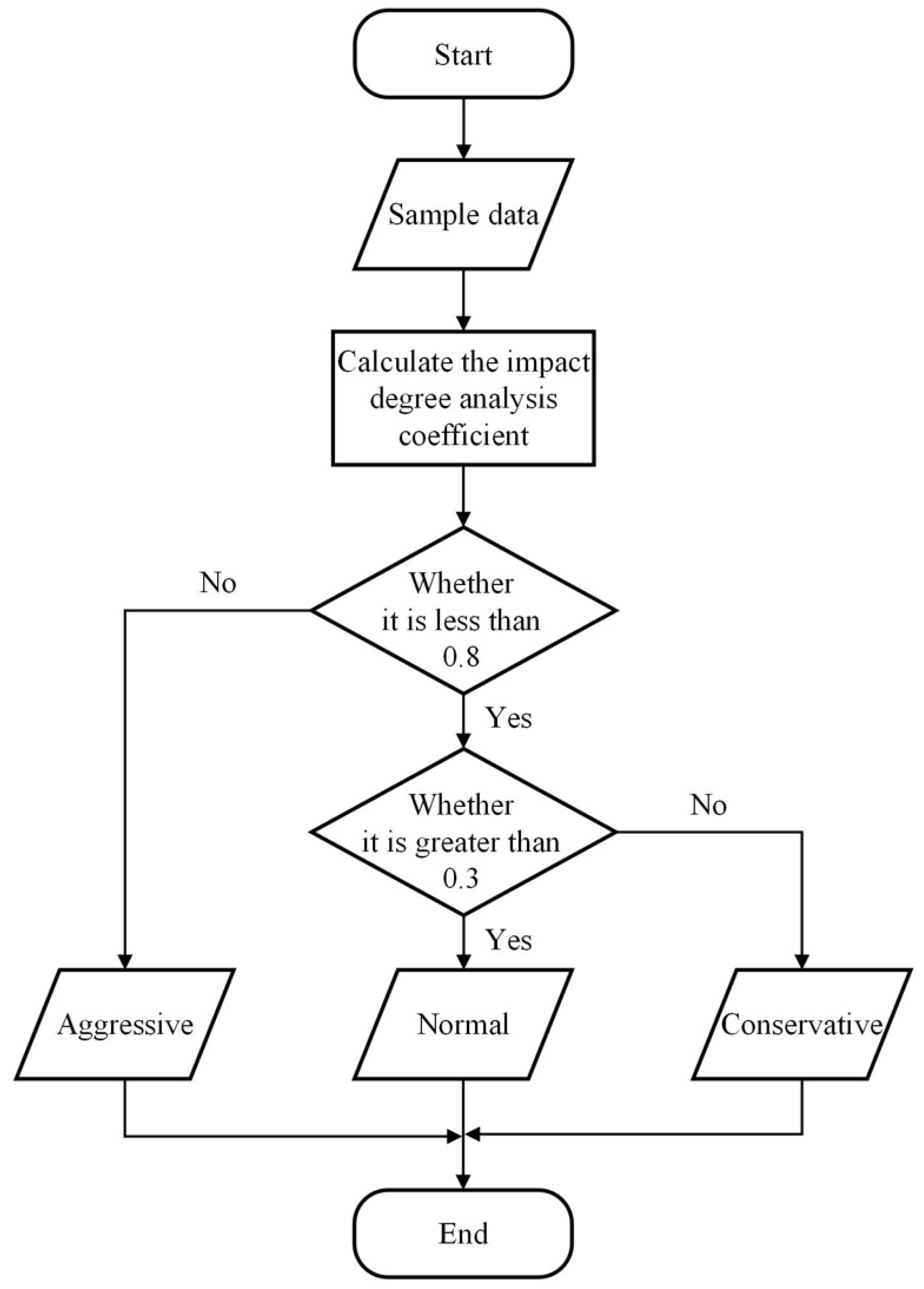
In Equation (15), the torque change rate of the driving motor affects the vehicle acceleration change rate (impact degree). In this section, the driving style of the driver is identified through the overall impact degree of the vehicle. The driving style recognition process is shown in Figure 3.

After the vehicle is in operation, time T is selected as the recognition period. In this study, T is taken as 200 s. Extract the vehicle speed information within the recognition period and conduct impact degree analysis. The impact degree J is shown in (23). Since the average impact degree cannot well reflect the fluctuation of the impact degree, the impact degree analysis coefficient R_driver is introduced. By using the normal deviation of the impact degree and the average absolute value of the impact degree, the impact degree of vehicles can be better analyzed.

The shift shock degree can be expressed by the differential of the vehicle’s longitudinal acceleration:

$$J={\displaystyle \frac{da}{dt}}={\displaystyle \frac{d^{2}v}{d{t}^2}}$$

(23)

where J is the vehicle impact degree; a represents the longitudinal acceleration of the vehicle.

Vehicle impact degree analysis formula:

$$R_{driver}={\displaystyle \frac{S{D}_J}{\overline{J}}}={\displaystyle \frac{\sqrt{\frac{1}{T}{\displaystyle \sum _{i=1}^T{\left(J_i-\frac{1}{T}{\displaystyle \sum _{i=1}^T{J}_i}\right)}^2}}}{\frac{1}{T}{\displaystyle \sum _{i=1}^T|}{J}_i|}}$$

(24)

where J_i is the instantaneous impact degree; SD_J is the normal deviation of the impact degree; and $\overline{J}$ is the average absolute value of the impact degree.

R_norm and R_agg are the critical values for normal and aggressive driving styles, respectively. When R_driver is less than R_norm, it indicates that the current driving style is conservative. When R_driver is greater than R_norm and less than R_agg, it indicates that the current driving style is normal. When R_driver is greater than R_agg, it indicates that the current driving style is aggressive [27]. Based on the driving experience of heavy vehicles, R_norm is taken as 0.3 and R_agg as 0.8.

Next, take the vehicle speed corresponding to the recognition period T in the LA92 driving cycle as the input, and then analyze the impact degree according to the driving style recognition process shown in Figure 4, which determines that the driver’s driving style is a “conservative driving style”.

3.3. Vehicle Speed Prediction Model Based on the Markov Chain Model

By predicting the future speed of the vehicle, AMT can adjust the gear shifting plan in advance to ensure that gear shifting occurs at the optimal time, thereby improving gear shifting efficiency, reducing energy consumption, and lowering exhaust emissions [28].

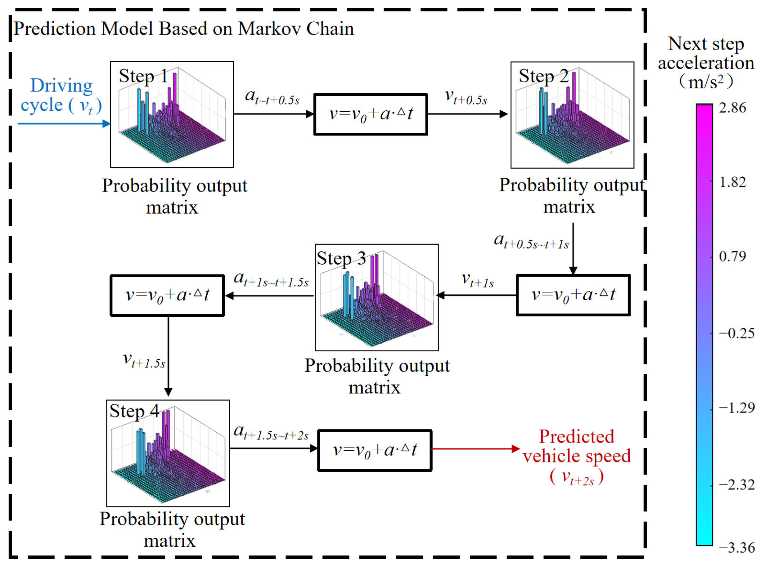
In situations such as climbing, speed prediction can help AMT downshift ahead to provide more power output. In certain emergency situations, such as the need for rapid acceleration or evasive maneuvers, speed prediction can ensure that the transmission responds ahead, thereby enhancing driving safety. The Markov chain principle can be utilized to calculate the driving cycle data and complete the speed prediction. Figure 5 shows the flowchart of speed prediction. The speed signal is collected and input into the probability output matrix of the four-stage Markov chain model to output the acceleration signal with the highest probability. The obtained acceleration is then substituted into Equation (25) to obtain the speed signal for the next stage.

$$v=v_0+a\mathrm{\Delta }t$$

(25)

The specific process of vehicle speed prediction is shown in Figure 5. According to the process, the predicted speed at 0.5, 1, 1.5, and 2 s later can be calculated successively. The implementation steps are as follows:

(1)

Input the current speed vt of the driving cycle into the probability output matrix of the first-stage Markov chain model to obtain the acceleration at ~t + 0.5 s from t to t + 0.5 s. Then, substitute it into Equation (25) to predict the speed vt + 0.5 s at t + 0.5 s.

(2)

Input vt + 0.5 s into the probability output matrix of the second-stage Markov chain model to obtain the acceleration at +0.5 s~t + 1 s from t + 0.5 s to t + 1 s. Then, substitute it into Equation (25) to predict the speed vt + 1 s at t + 1 s.

(3)

Input vt + 1 s into the probability output matrix of the third-stage Markov chain model to obtain the acceleration at +1 s~t + 1.5 s from t + 1 s to t + 1.5 s. Then, substitute it into Equation (25) to predict the speed vt + 1.5 s at t + 1.5 s.

(4)

Input vt + 1.5 s into the probability output matrix of the fourth-stage Markov chain model to obtain the acceleration at +1.5 s~t + 2 s from t + 1.5 s to t + 2 s. Then, substitute it into Equation (25) to predict the speed vt + 2 s at t + 2 s.

To calculate the probability output matrix of the Markov chain model, 10 typical driving cycles, namely INDIA_URBAN_SAMPLE, UDDS, WVUSUB, MANHATTAN, NurembergR36, NYCC, WVUCITY, HWFET, NREL2VAIL, and US06_HWY, were selected as sample data to calculate the probability output matrix of the Markov chain model [29]. To build a high-order Markov chain model, it is necessary to calculate the probability distribution matrix of vehicle acceleration corresponding to different vehicle speeds in these 10 driving cycles. Equation (26) is used:

$$\begin{array}{l}{p}_{i_1,i_2,i_3\dots i_s,j}=P\left\{\begin{array}{l}a(t+n)={\overline{a}}_j|v(t+n-0.5)={\overline{v}}_{i_1},v(t+n-1)={\overline{v}}_{i_2},\hfill \\ \hspace{1em}\hspace{1em}\dots v(t+n-2)={\overline{v}}_{i_s}\hfill \end{array}\right\}\\ i,j=1,2,\dots ,m;n=0.5,1,\dots ,L_{PH};\end{array}$$

(26)

where s is the order of the Markov chain model; m is the number of states; n is the time point in the prediction time domain; and L_PH is the length of the prediction time domain.

The vehicle speed and acceleration curves of the sample data are discretized and analyzed using the clustering analysis algorithm. The sample vehicle speed curves are discretized into N intervals from small to large, with the unit of speed being m/s, and the value of each interval is v_i, as shown in Equation (27):

$$v_i=\{v_1,v_2,\dots ,v_N\}$$

(27)

where N is set to 30.

The acceleration curves are discretized into M intervals from small to large, and the value of each interval is a_j, as shown in Equation (28):

$$a_j=\{a_1, a_2,\dots , a_M\}$$

(28)

where M is set to 30.

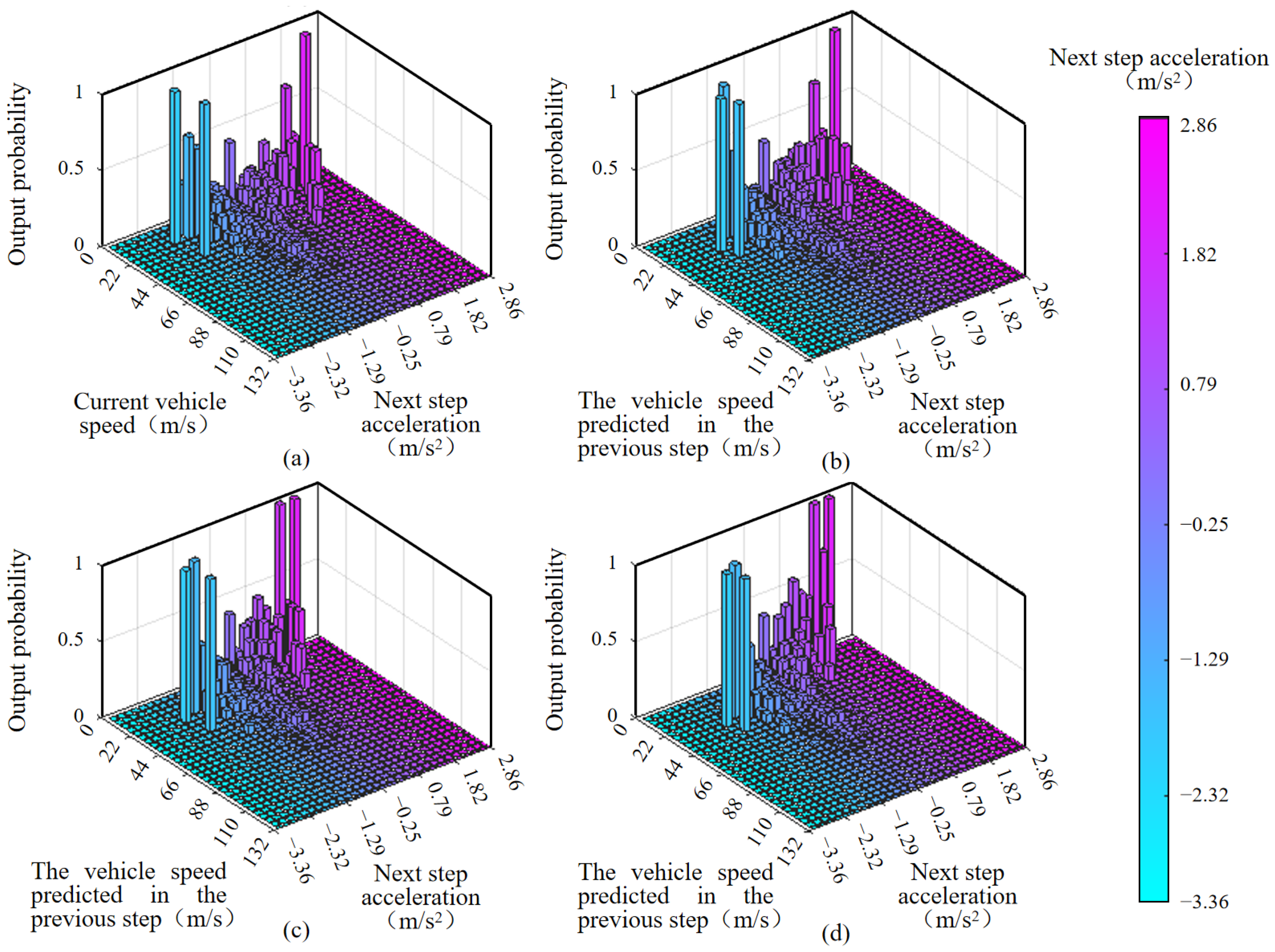
The Markov chain probability output matrix is divided into four stages, and the average acceleration in the next 0.5 s is predicted in each stage to achieve better prediction results. Figure 6a–d present the probability output matrices of the Markov chain model in the four stages. The calculation process is as follows:

(1)

Calculation of the probability output matrix of the first stage of the Markov chain model: The vehicle speed at time t was input based on the sample data, and then the probability distribution of acceleration from t to t + 0.5 s in the sample data was determined.

(2)

Calculation of the probability output matrix of the second stage of the Markov chain model: The vehicle speed at time t + 0.5 s was calculated by the probability output matrix of the first stage of the Markov chain model. The vehicle speed at time t + 0.5 s was input, and then the probability distribution of acceleration from t + 0.5 s to t + 1 s in the sample data was determined.

(3)

Calculation of the probability output matrix of the third stage of the Markov chain model: The vehicle speed at time t + 1 s was calculated by the probability output matrix of the second stage of the Markov chain model. Then, the vehicle speed at time t + 1 s was analyzed to find the probability distribution of acceleration from t + 1 s to t + 1.5 s in the sample data.

(4)

Calculation of the probability output matrix of the fourth stage of the Markov chain model: The vehicle speed at time t + 1.5 s was calculated by the probability output matrix of the second stage of the Markov chain model. Then, the vehicle speed at time t + 1.5 s was analyzed to find the probability distribution of acceleration from t + 1.5 s to t + 2 s in the sample data.

After inputting the vehicle speed into the probability output matrix of the Markov chain model, the probability distribution of the acceleration corresponding to the discretized vehicle speed v_i is calculated. The discretized acceleration signal a_j corresponding to the maximum probability is the predicted acceleration signal. Equation (29) is used:

$${\widehat{X}}_t=j , \mathrm{if} {[{\widehat{X}}_t]}_i\le {[{\widehat{X}}_t]}_j , \forall i,j=\{1,2,\dots ,N\}$$

(29)

where ${\widehat{X}}_t$ is the state with the maximum probability; m represents the number of states and is set to 30.

After predicting the acceleration signal, the vehicle speed prediction can be completed according to the specific process shown in Figure 5, and the vehicle speed in the next 2 s, namely the “Predicted vehicle speed”, can be obtained.

3.4. Adaptive Shift Model Based on Fuzzy Control

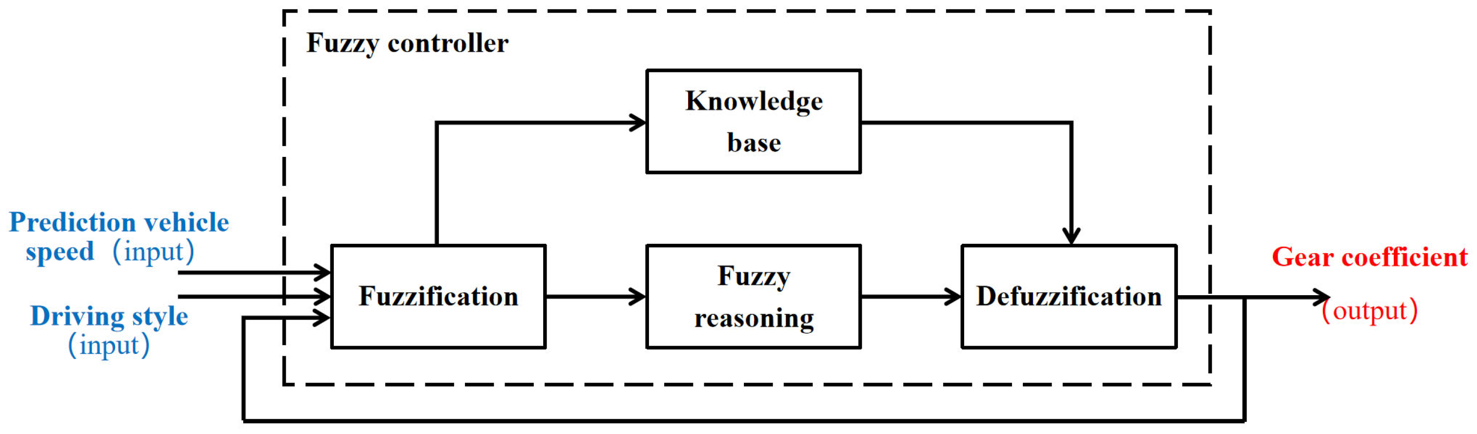
In the shift decision-making process shown in Figure 3, fuzzy control serves as the link to the control strategy, which can adapt to different operating conditions and environmental changes, and it has good flexibility and adaptability. At the same time, the fuzzy control system can resist the influence of factors such as parameter changes and external disturbances to a certain extent, and it has good robustness [30]. Therefore, in order to conform to the driver’s driving habits and take advantage of vehicle speed prediction and fuzzy control, a fuzzy controller is designed, and a shift strategy that meets the driver’s needs is formulated. The formulated fuzzy control process is shown in Figure 7. As shown in Figure 7, in the formulated shift strategy, the “predicted road conditions” and “driving style” are taken as inputs, and the required gear coefficient is output through the built fuzzy controller.

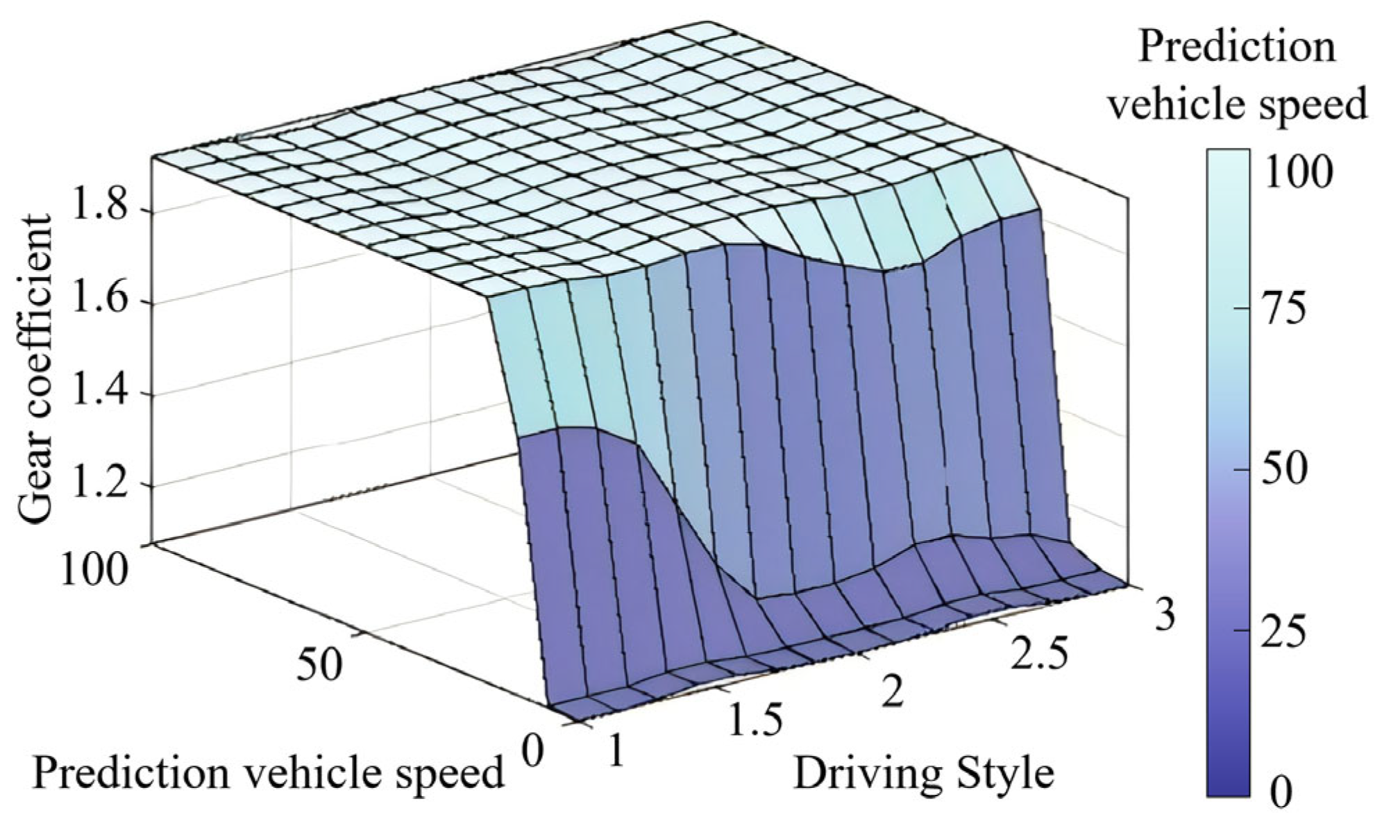
The gear ratio coefficient is not necessarily an integer. In the gear shifting strategy, it represents the driver’s demand for the target gear. To output the corresponding gear ratio coefficient according to different predicted operating conditions and driving styles, “Fuzzy Rule 1,” as shown in Figure 8, was formulated. In the fuzzy rule, the speed range of the “predicted operating conditions” is selected as “0~100 m/s”. Since there are three different driving styles, the numerical range of the “driving style” is selected as “1~3”. As the research object is a two-speed AMT for electric heavy-duty vehicles, the gear positions of the transmission are two, so the numerical range of the gear ratio coefficient is “1~2”.

In the “Driving Style” coordinate axis of Figure 8, “Conservative Driving Style” is represented by the number 1, “Normal Driving Style” by the number 2, and “Aggressive Driving Style” by the number 3. According to the inputs “Predicted driving condition” and “Driving Style”, the corresponding gear ratio coefficient can be output based on the above fuzzy rules.

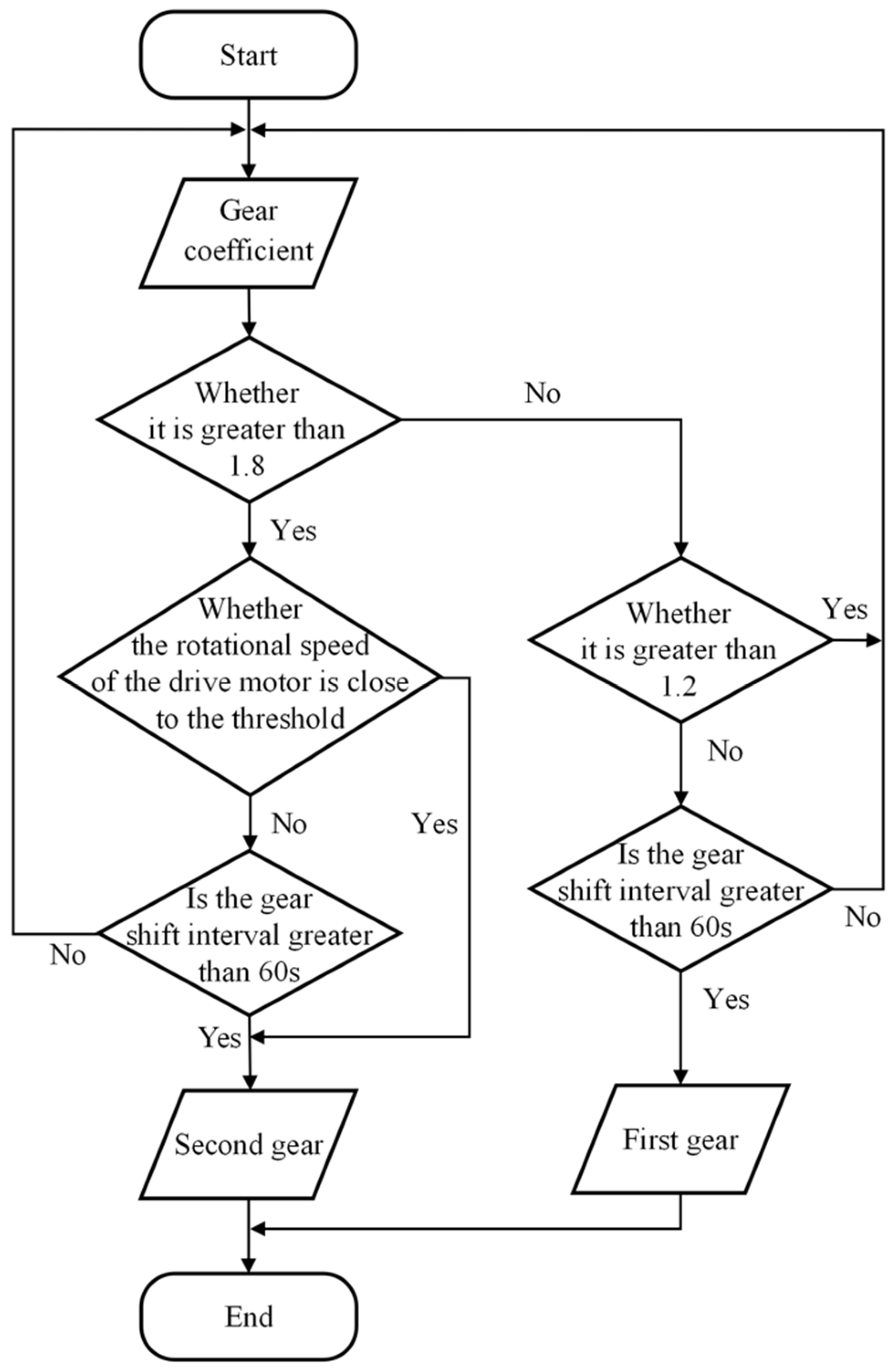
To avoid the problem of frequent gear shifting in conventional shifting strategies, this paper designs an adaptive adjustment strategy. Figure 9 presents the flowchart of the adaptive adjustment. The adaptive adjustment strategy records the interval time of each gear shift, collects the vehicle speed signal, and calculates the drive motor speed based on the vehicle speed and gear signal. Finally, the target gear is determined based on the drive motor speed, the interval time of gear shifting, and the gear ratio coefficient. The relationship between vehicle speed and drive motor speed is shown in Equation (30):

v = 2πr·n_d·i

(30)

where r is the wheel rolling radius; n is the drive motor speed; and i is the transmission ratio.

Since the transmission ratio of the transmission varies with different gears, when calculating the drive motor speed, the corresponding transmission ratio i should be substituted into Equation (30) according to different gear signals.

The summary of the target gear output scheme is as follows:

(1)

When the gear coefficient output by the fuzzy controller is greater than 1.8 and the motor speed is close to the maximum speed, the target gear is adjusted to the second gear.

(2)

When the gear coefficient output by the fuzzy controller is greater than 1.8 and the shift interval is more than 60 s, the target gear is adjusted to the second gear.

(3)

When the gear coefficient output by the fuzzy controller is greater than 1.2 and less than 1.8, the target gear remains unchanged.

(4)

When the gear coefficient output by the fuzzy controller is less than 1.2 and the shift interval is more than 60 s, the target gear is adjusted to the first gear.

3.5. Shift Model Construction Based on Speed and Its Rate of Change

In this paper, the speed difference and the rate of change in the speed difference are collected to improve the fuzzy rules. The research object in this paper is a two-speed AMT for electric heavy-duty vehicles. The transmission used allows engagement with a relatively large speed difference. In this paper, it is set that when the speed difference is within 1500 r/min, the synchronizer can start to engage.

Since the speed of the drive motor is related to the opening degree of the accelerator pedal, the rate of change in the speed of the drive motor is also related to the speed at which the driver steps on the accelerator or brake pedal. When the rate of change in vehicle speed is relatively large, it indicates that the driver is in a hurry. When the rate of change is relatively small, it indicates that the driver is driving smoothly. The purpose of collecting the speed difference and the rate of change in the speed difference is to output the speed of the shift motor that meets the driver’s requirements, but it can only roughly reflect the driver’s intention and cannot precisely output the speed of the shift motor. Therefore, this paper proposes the speed demand coefficient of variable-speed motors.

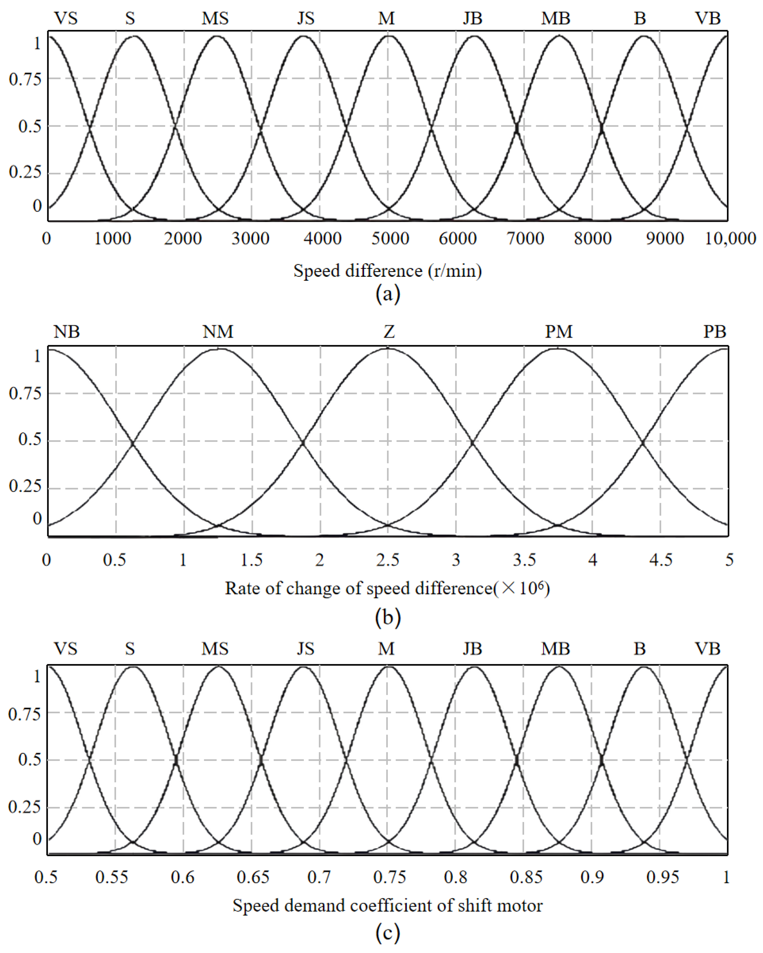
The shift motor speed demand coefficient is a number between 0 and 1 that is multiplied by the shift motor speed before the output in this paper. The function of the shift motor speed demand coefficient is to adjust the shift motor speed to better complete the shift. Taking the rate of change in the speed difference and the speed difference of the two friction gears during the synchronization process as the input of fuzzy controller 2, and taking the shift motor speed demand coefficient as the output, and then establishing a complete set of fuzzy rules, the optimization of the shift force can be achieved. Fuzzy rule 2 is shown in

Table 3. Fuzzy rules 2.

Drive the Motor Speed Demand Coefficient		Speed Difference
		VS	S	MS	JS	M	JB	MB	B	VB
Rate of change in speed difference	NB	VS	S	MS	JS	M	JB	MB	VB	VB
	NM	VS	S	JS	M	JB	MB	B	VB	VB
	Z	S	MS	JS	M	JB	MB	VB	VB	VB
	PM	VS	S	JS	M	JB	MB	B	VB	VB
	PB	VS	S	MS	JS	M	JB	MB	VB	VB

. The range of the speed difference is 0 to 10,000 r/min, and the rate of change in the speed difference is taken as the ratio of the speed difference to 0.002, with a numerical range of 0 to 5,000,000. The speed difference of the two gears on both sides of the synchronizer during the synchronization process is taken as the absolute value, and the minimum time interval of the fuzzy controller is taken as 0.002 s. The specific situation is as follows:

(1)

Speed difference (0, 10,000): very small (VS), small (S), medium–small (MS), relatively small (JS), medium (M), relatively large (JB), medium–large (MB), large (B), and very large (VB)

(2)

Rate of change in speed difference (taking the speed change rate of 0.002 s) (0, 5,000,000): small (NB), relatively small (NM), medium (Z), relatively large (PM), and large (PB).

(3)

Shift motor speed demand coefficient (0.5, 1): very small (VS), small (S), medium–small (MS), relatively small (JS), medium (M), relatively large (JB), medium–large (MB), large (B), and very large (VB).

To better present the fuzzy rules, the fuzzy rule curve graph of Figure 10 was drawn. This paper adopts the Gaussian membership function (gaussmf), and the curve of the Gaussian distribution has the advantage of a smooth transition. To formulate the fuzzy rules, import them into fuzzy controller 2. Then, multiply the output speed demand coefficient of the shift motor by the speed of the shift motor to optimize the speed of the shift motor, which meets the driver’s requirements.

The PID controller is as follows [31]:

$$u(t)=K_{p}e(t)+K_i{\displaystyle {\int }_0^{t}e}(\tau )d\tau +K_d{\displaystyle \frac{de(t)}{dt}}$$

(31)

where u(t) denotes the controller output signal, e(t) represents the error between the desired setpoint and the measured process variable, and K_p, K_i, and K_d are the proportional, integral, and derivative gain coefficients, respectively.

Using the shift motor as the controlled object, the position of the shift fork is regulated by adjusting the motor’s rotational speed, thus enabling precise control over shift displacement. The deviation between the actual shift displacement and the target displacement serves as the feedback error, which is fed into the PID controller to achieve closed-loop control. As shown in Figure 11, this configuration constitutes the schematic of the PID control structure.

During the PID control process, the speed of the shift motor is converted into linear displacement via mechanical transmission. The conversion relationships are defined in Equations (32)–(34):

$${\theta }_D={\displaystyle {\int }_0^T{\omega }_D}dt$$

(32)

$${\theta }_B={\theta }_D/n_H$$

(33)

$$x_D=l_B\sin {\theta }_B$$

(34)

where θ_D denotes the rotation angle of the shift motor; ω_D represents its angular velocity; n_H is the gear reduction ratio (set to 54); x_D is the linear shift displacement; l_B is the length of the fork arm; and θ_B is the angle between the fork arm and the vertical axis.

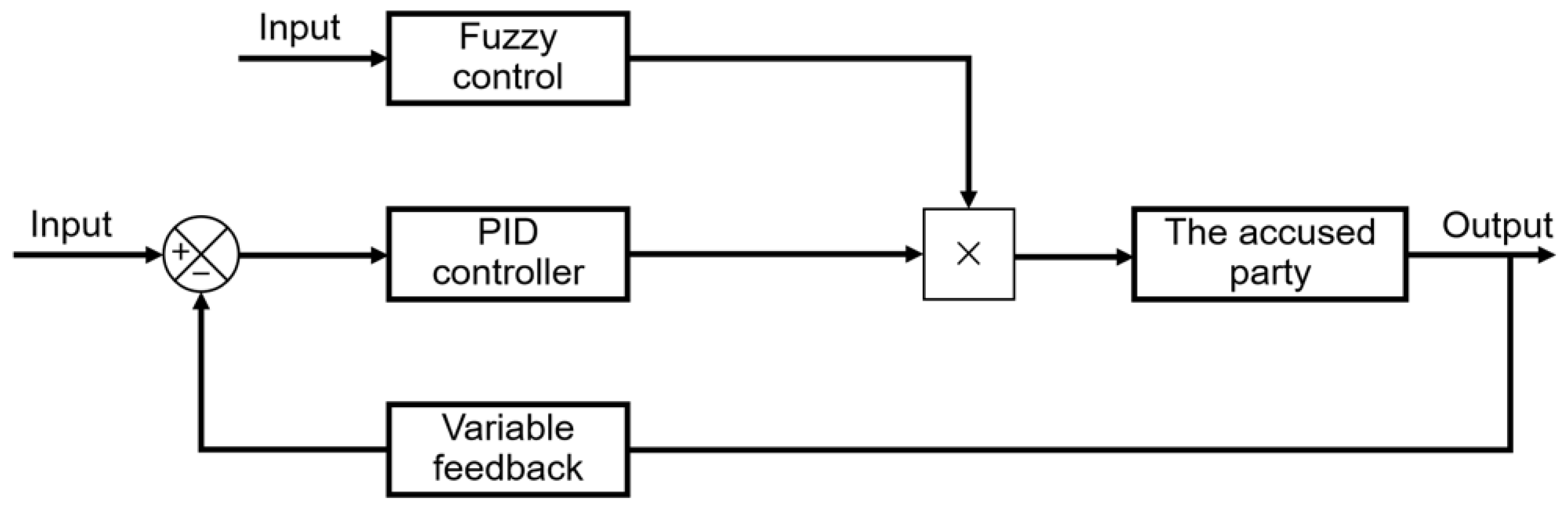
To enhance the responsiveness and adaptability of the shift actuator control, the previously described fuzzy controller is combined with the PID controller, forming a hybrid fuzzy PID control system. The architecture of the proposed fuzzy PID controller is illustrated in Figure 12.

The fuzzy controller operates independently from the PID controller, rather than dynamically tuning the K_p, K_i, and K_d parameters according to fuzzy rules. This decoupled design enables the shifting motor to shift based on the speed demand coefficient. The aim is to operate in accordance with real-time driver intentions.

4. Simulation and HIL Testing

Section 4 presents a comparative analysis conducted in the MATLAB/Simulink environment using driving cycles to evaluate the performance of the optimized control model against both the conventional approach and the adaptive shift schedule design method presented in [14]. Additionally, experimental validation was performed on a HIL testing for the shift motor to verify the feasibility of optimizing the shift execution process through speed regulation.

4.1. Simulation

4.1.1. Analysis of Vehicle Speed Prediction in Driving Cycles

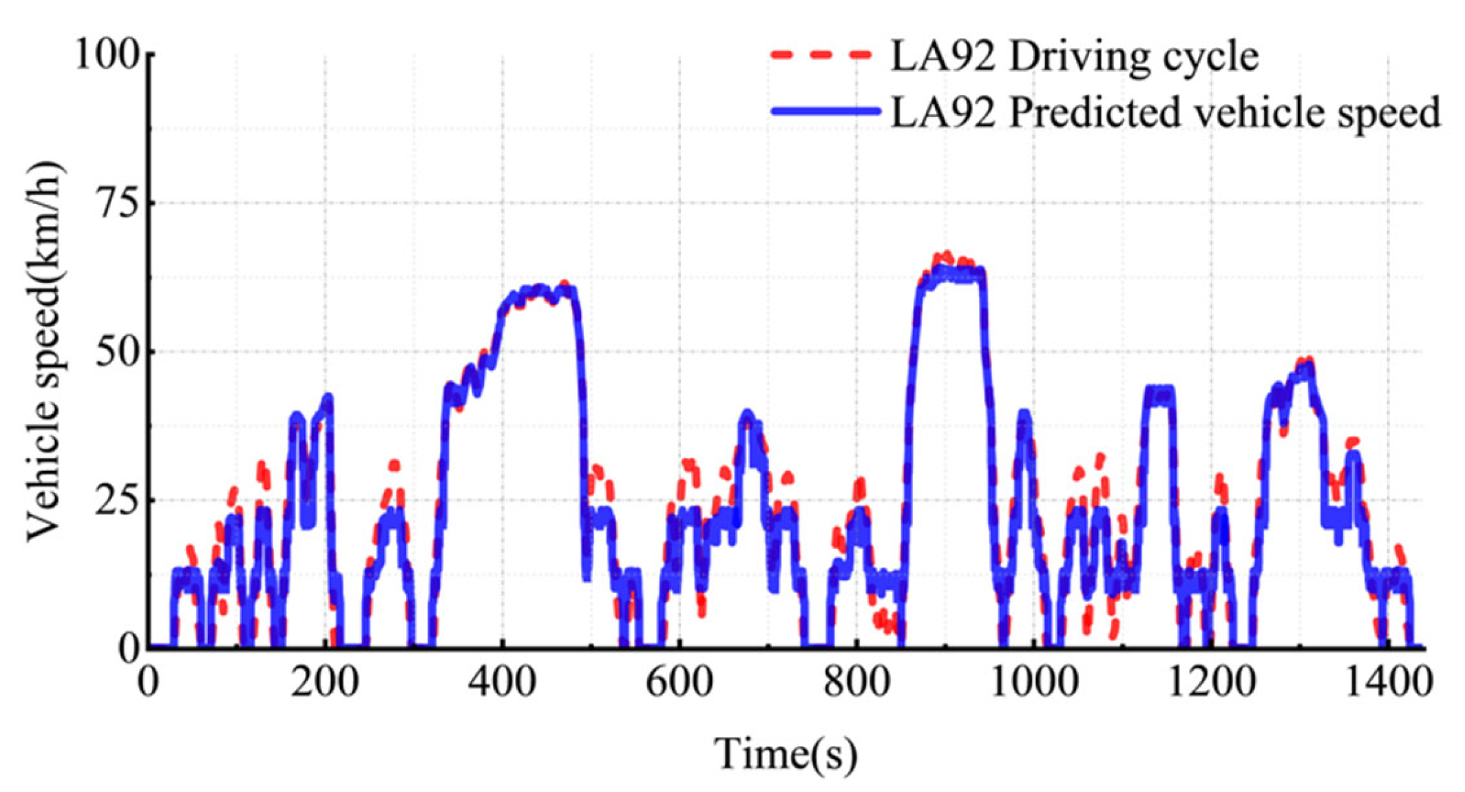
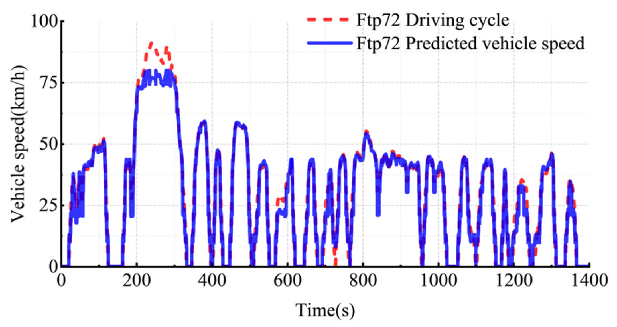
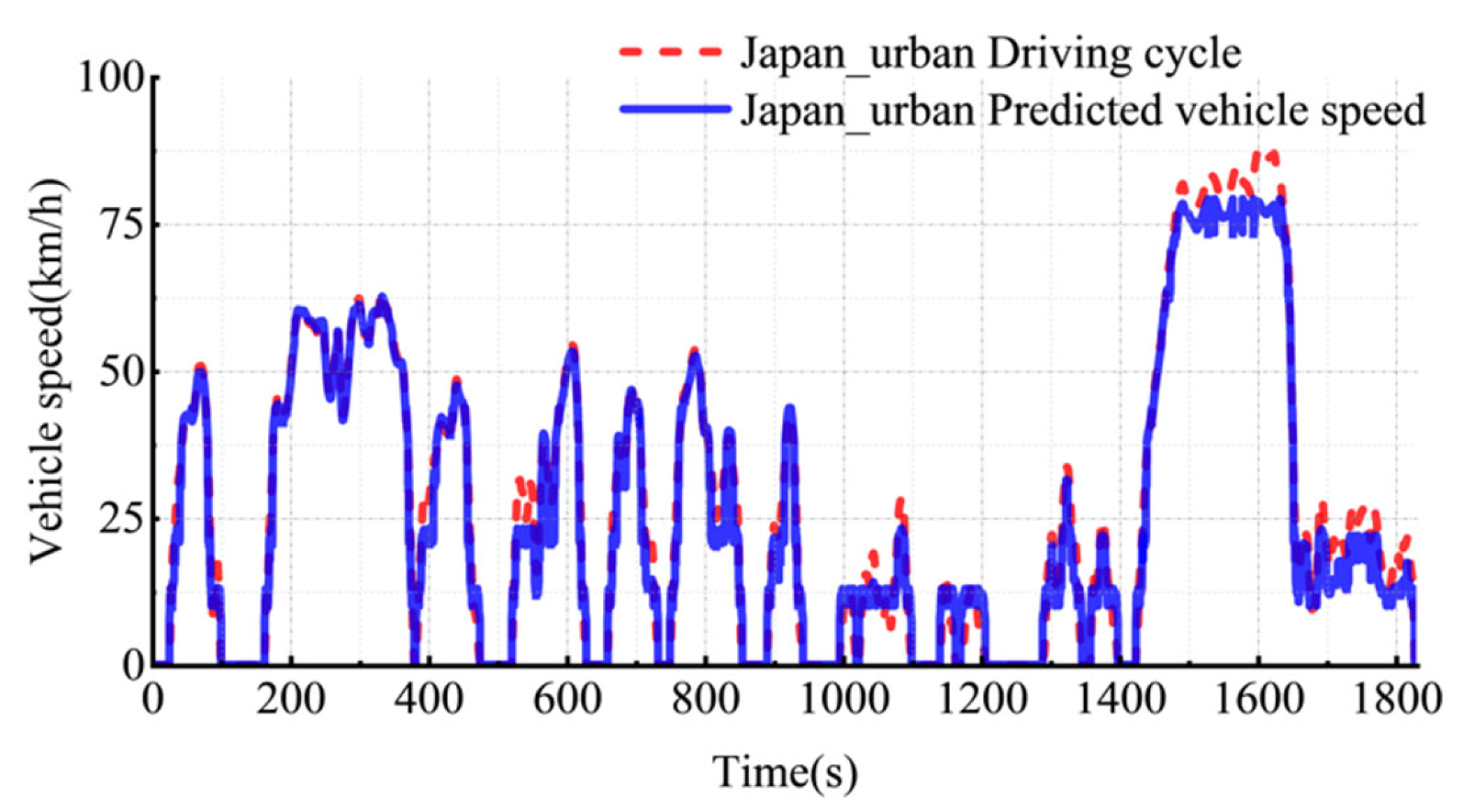
To investigate the adaptive shifting strategy, the LA92, Ftp72, and Japan_urban driving cycles were selected for analysis. Predicted vehicle speed profiles under these driving cycles serve as inputs to the fuzzy controller in subsequent simulations. Figure 13, Figure 14 and Figure 15 illustrate the actual driving cycles and their corresponding predicted speed trajectories.

In Figure 13, Figure 14 and Figure 15, the red dashed line labeled “Driving cycle” is the original vehicle speed, while the blue solid line labeled “Predicted vehicle speed” is the predicted vehicle speed. It can be observed that the prediction accuracy decreases during periods of rapid speed fluctuation. At a relatively stable speed, the prediction error remains within 5%. It is worth noting that the LA92, Ftp72, and Japan_urban driving cycles were not used to develop the speed prediction model. Nevertheless, the model demonstrates strong speed prediction capability, indicating robust predictive performance beyond the sample data.

4.1.2. Shift Frequency Comparison

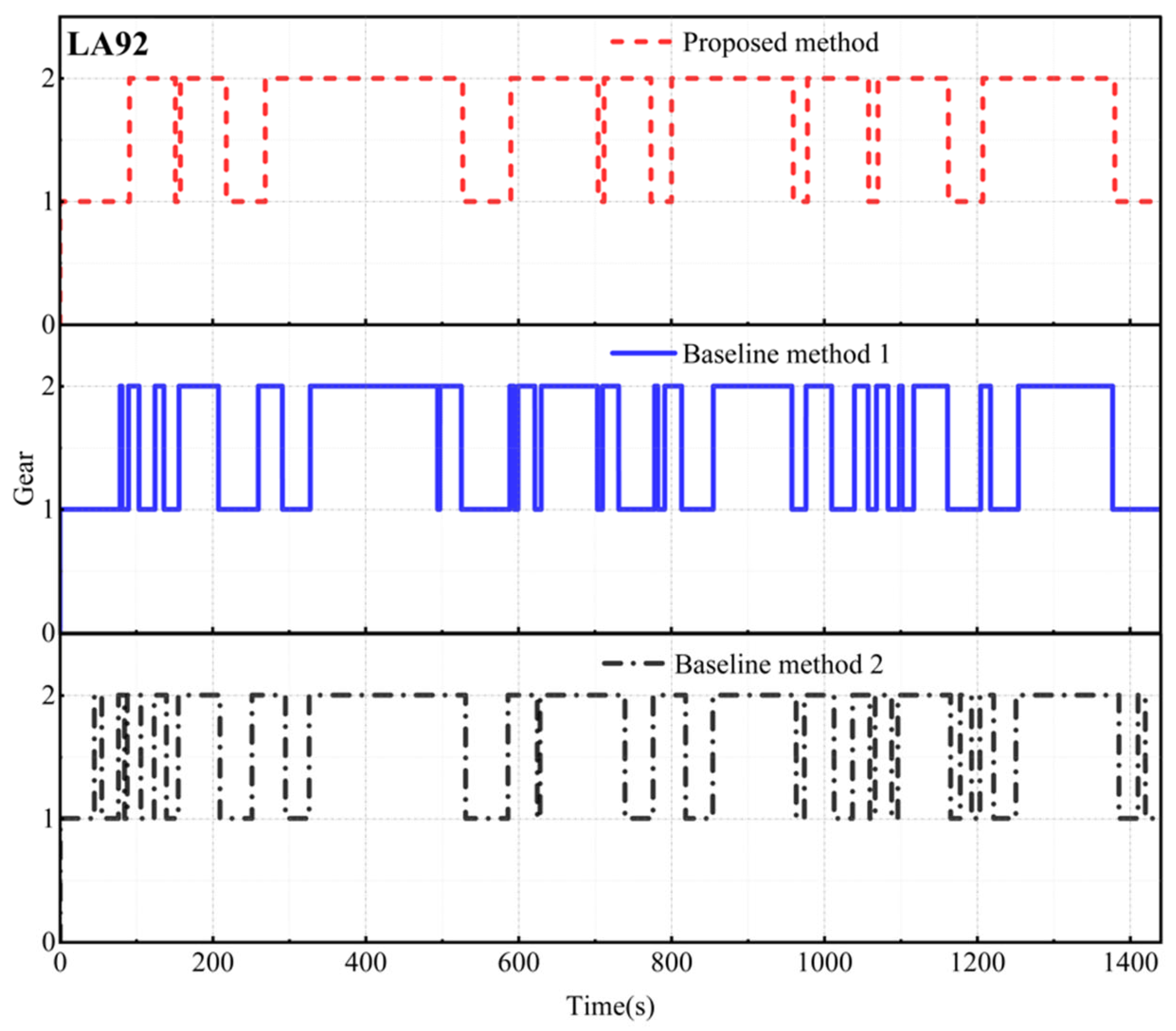
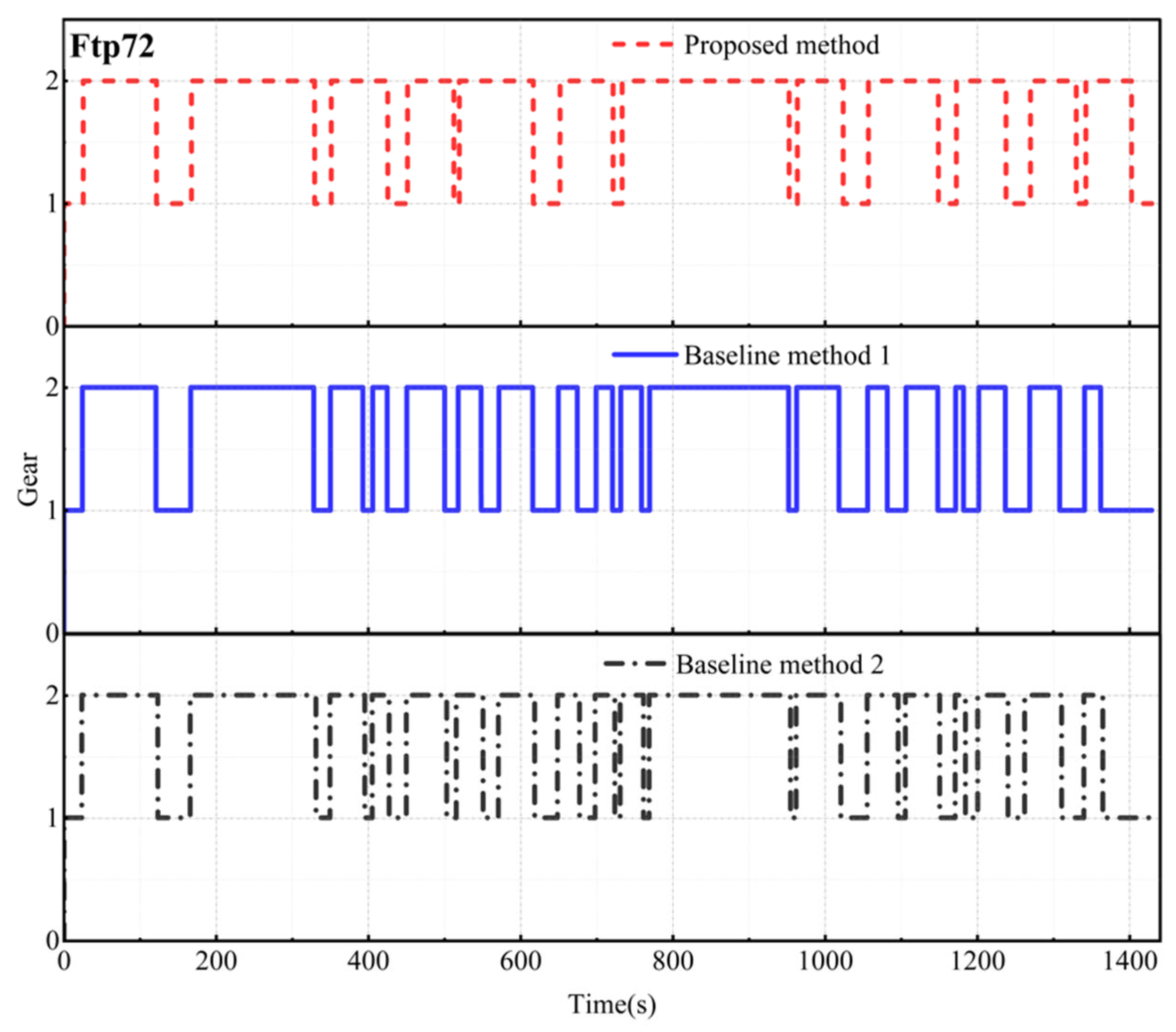
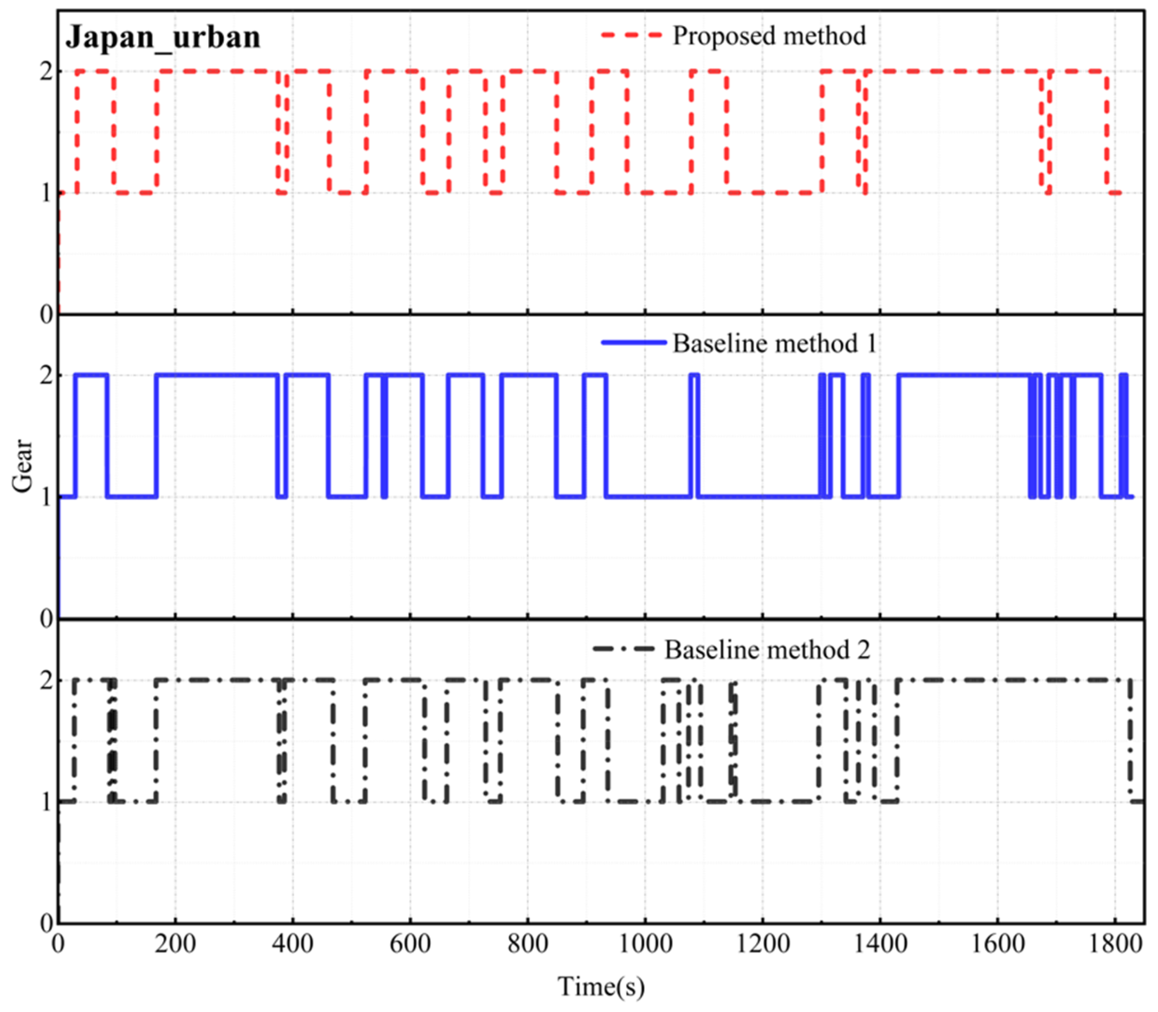
To verify the effect of the optimized shift control model in avoiding frequent gear shifts. This paper takes driving cycles as variables to study the shifting frequencies of the same driving cycle under various shifting strategies. The optimization strategy of this article is designated as the proposed method, the conventional strategy is designated as baseline method 1, and the adaptive shift schedule design method from [14] is designated as baseline method 2.

The conventional method determines shift points based on vehicle speed. The adaptive method is an adaptive shift schedule design method for multi-gear AMT electric vehicles based on dynamic programming and fuzzy logical control.

As shown in Figure 16, Figure 17 and Figure 18, the shifting frequencies of the proposed method, baseline method 1, and baseline method 2 are compared over the LA92, Ftp72, and Japan_urban driving cycles.

Table 4. Shift frequency comparison.

	Proposed Method	Baseline Method 1	Baseline Method 2
LA92	18	42	38
Ftp72	23	36	36
Japan_urban	22	36	28

shows the comparison of the number of shifts. In the LA92 driving cycle, the shift frequency of the proposed method is reduced by 57.14% relative to baseline method 1 and by 52.63% relative to baseline method 2. In the Ftp72 driving cycle, the proposed method achieves a reduction of 36.11% in shift frequency compared to both baseline methods. In the Japan_urban driving cycle, the shifting frequency of the proposed method decreases by 38.89% compared to baseline method 1 and by 21.43% compared to baseline method 2.

The fuzzy PID gear shifting control strategy for electric vehicles based on driving style and vehicle speed prediction solves the problem of frequent gear shifting and avoids some negative impacts on drivers caused by frequent gear shifting.

4.1.3. Dynamic Performance Comparison

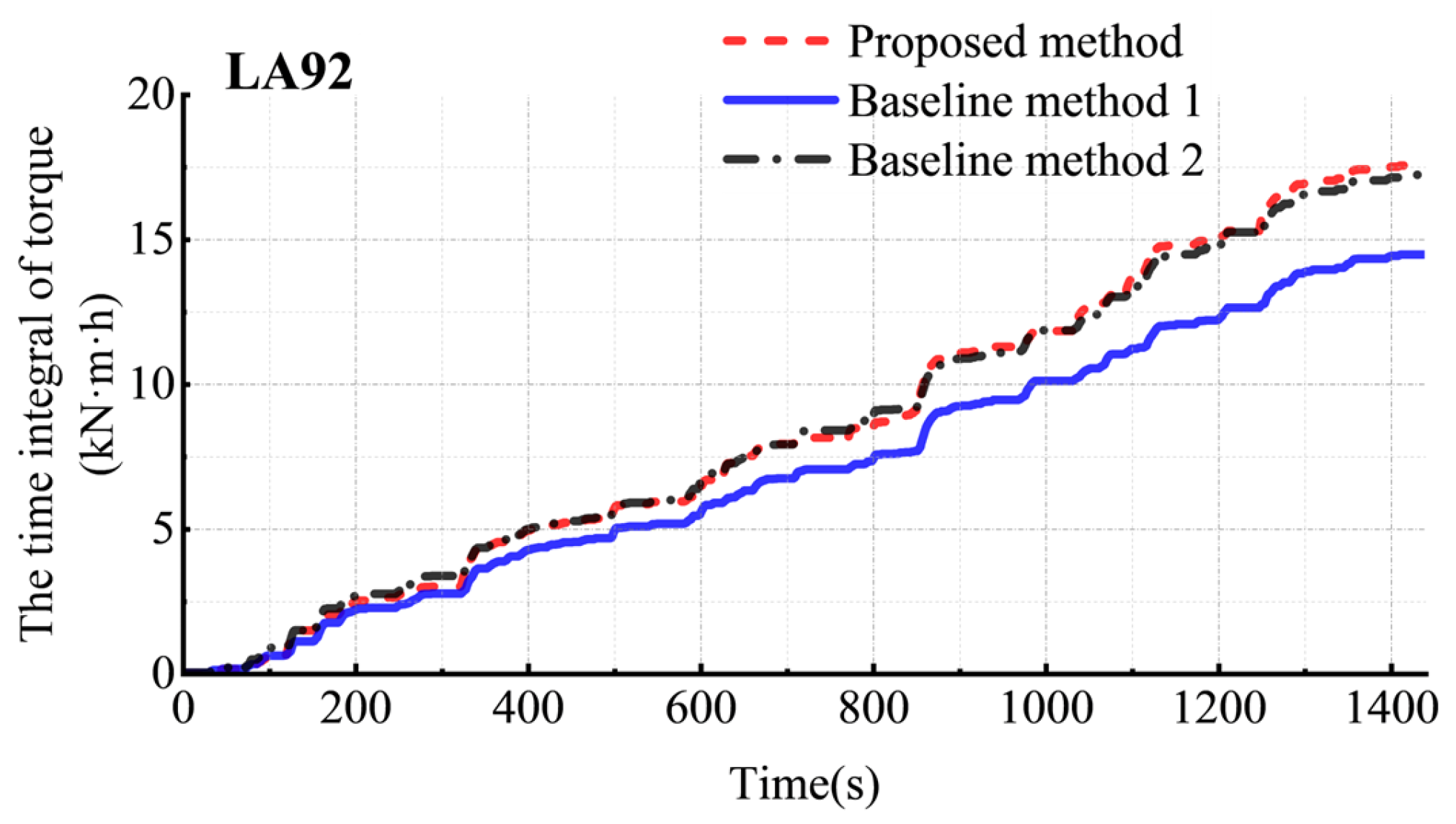
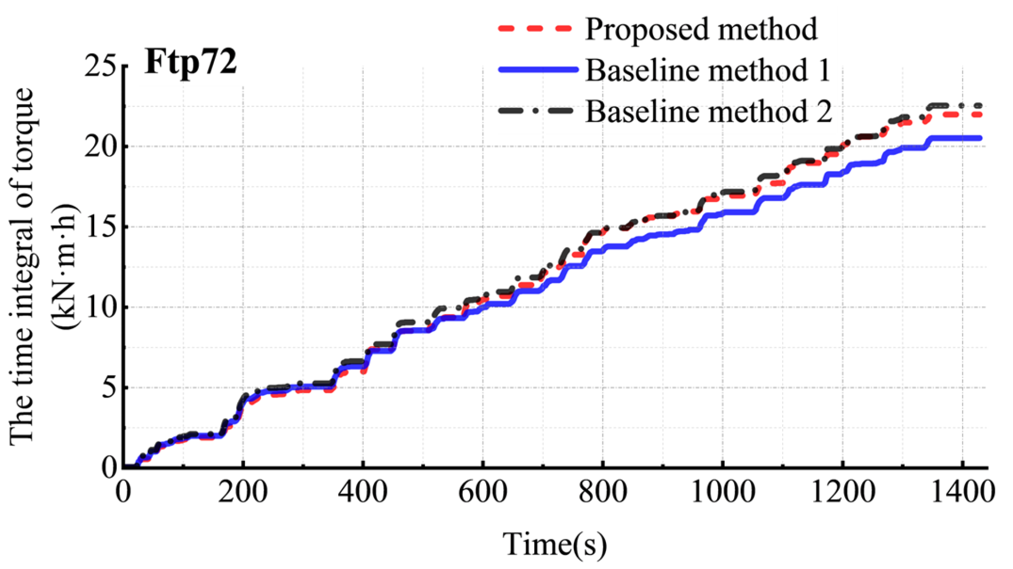
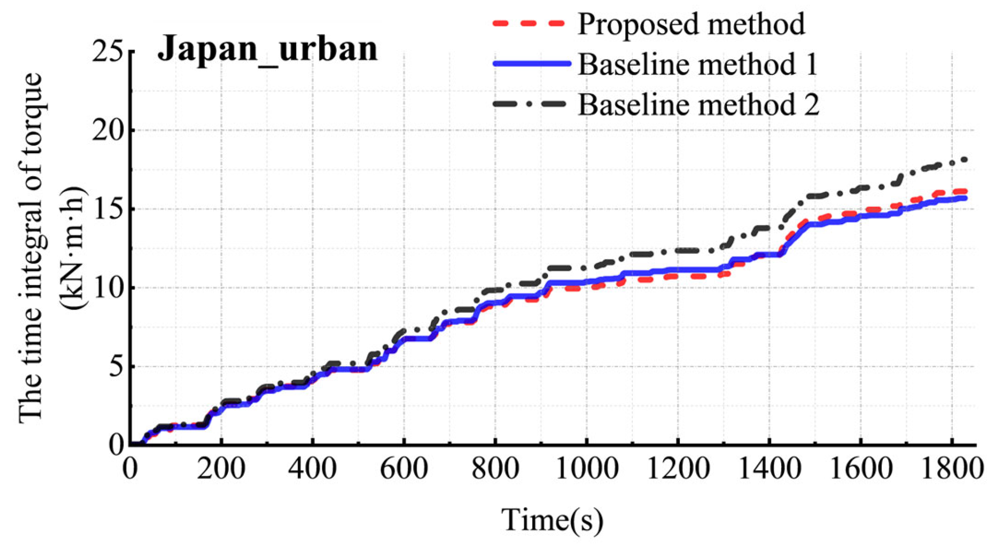
To evaluate the improvement of vehicle dynamic performance, the integral of torque over time is used as an indicator. Simulations were conducted in the LA92, Ftp72, and Japan_urban driving cycles to ensure reliability. The results are presented in Figure 19, Figure 20 and Figure 21.

Table 5. Dynamic performance comparison results.

	Proposed Method	Baseline Method 1	Baseline Method 2	Units
LA92	17.55	14.46	17.23	kN·m·h
Ftp72	21.97	20.51	22.52	kN·m·h
Japan_urban	16.10	15.67	18.12	kN·m·h

shows the dynamic performance comparison.

In the LA92 (Figure 19), Ftp72 (Figure 20), and Japan_urban (Figure 21) driving cycles, the time integral of torque values for baseline method 1 are 14.46, 20.51, and 15.67 kN·m·h, respectively, while the corresponding values of the proposed method are 17.55, 21.97, and 16.10 kN·m·h, respectively. These values increase by 21.36%, 7.18%, and 2.74%, respectively, compared to baseline method 1. This indicates that, under the same vehicle speed, both acceleration and climbing performance of the proposed method are improved compared to baseline method 1. Overall, the dynamic performance of the proposed method is enhanced by 21.36%, 7.18%, and 2.74% compared to baseline method 1 in the LA92, Ftp72, and Japan_urban cycles, respectively.

The time integral of torque values for baseline method 2 are 17.23, 22.52, and 18.12 kN·m·h in the LA92, Ftp72, and Japan_urban driving cycles, respectively. In the LA92 driving cycle, the dynamic performance of the proposed method is 1.86% higher than that of baseline method 2. In the Ftp72 and Japan_urban driving cycles, the dynamic performance of the proposed method is 2.44% and 11.15% lower than that of baseline method 2, respectively. Compared with baseline method 2, the dynamic performance of the proposed method is higher in some cycles and lower in others, owing to the differences in the driving cycles.

4.1.4. Economic Performance Comparison

To assess the improvements in energy efficiency, simulations were conducted to compare the proposed strategy with both the conventional vehicle-speed-based method and the adaptive shift schedule design method reported in [14]. Key economic indicators include drive motor energy consumption and battery state of charge (SOC).

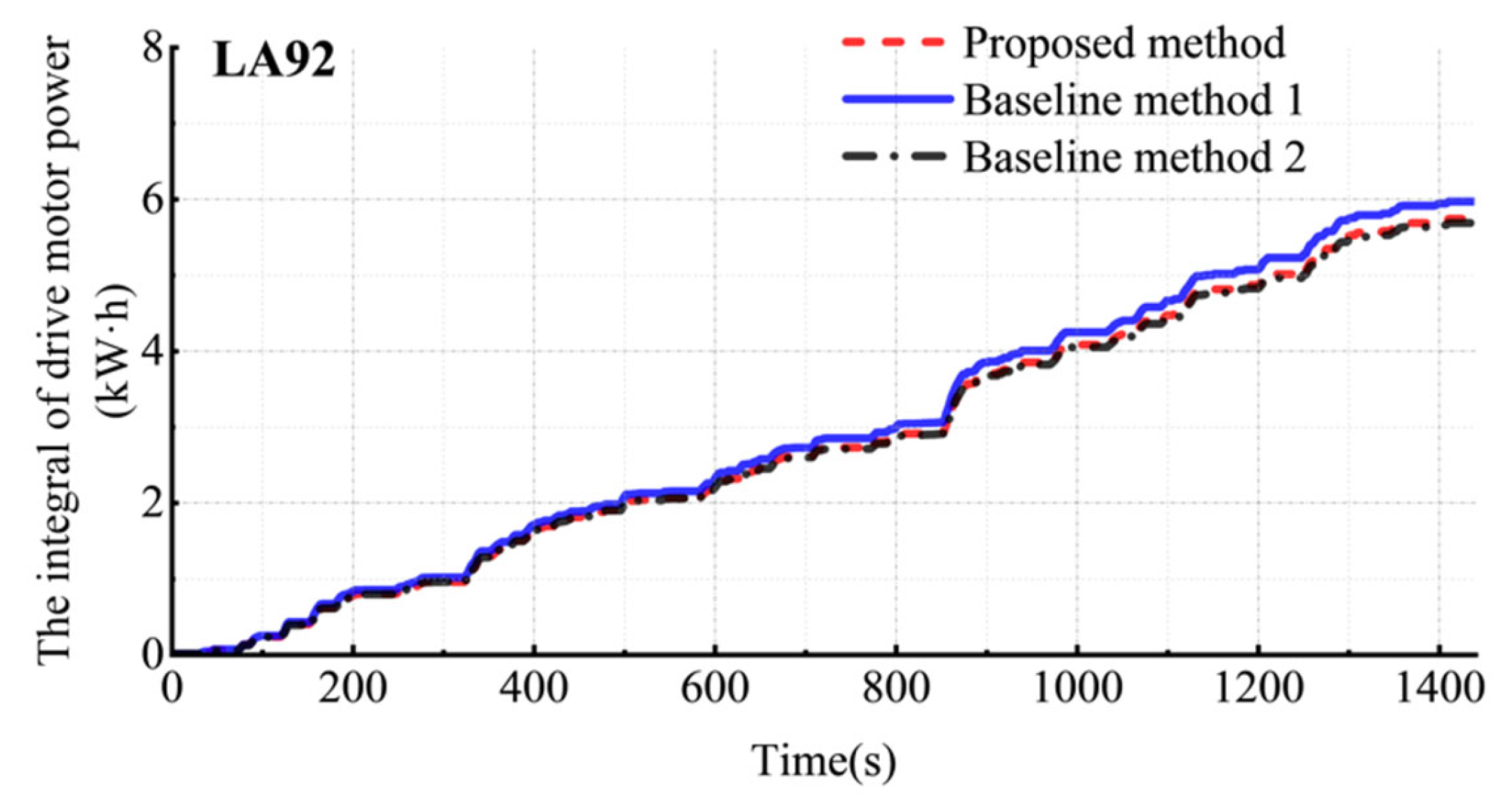
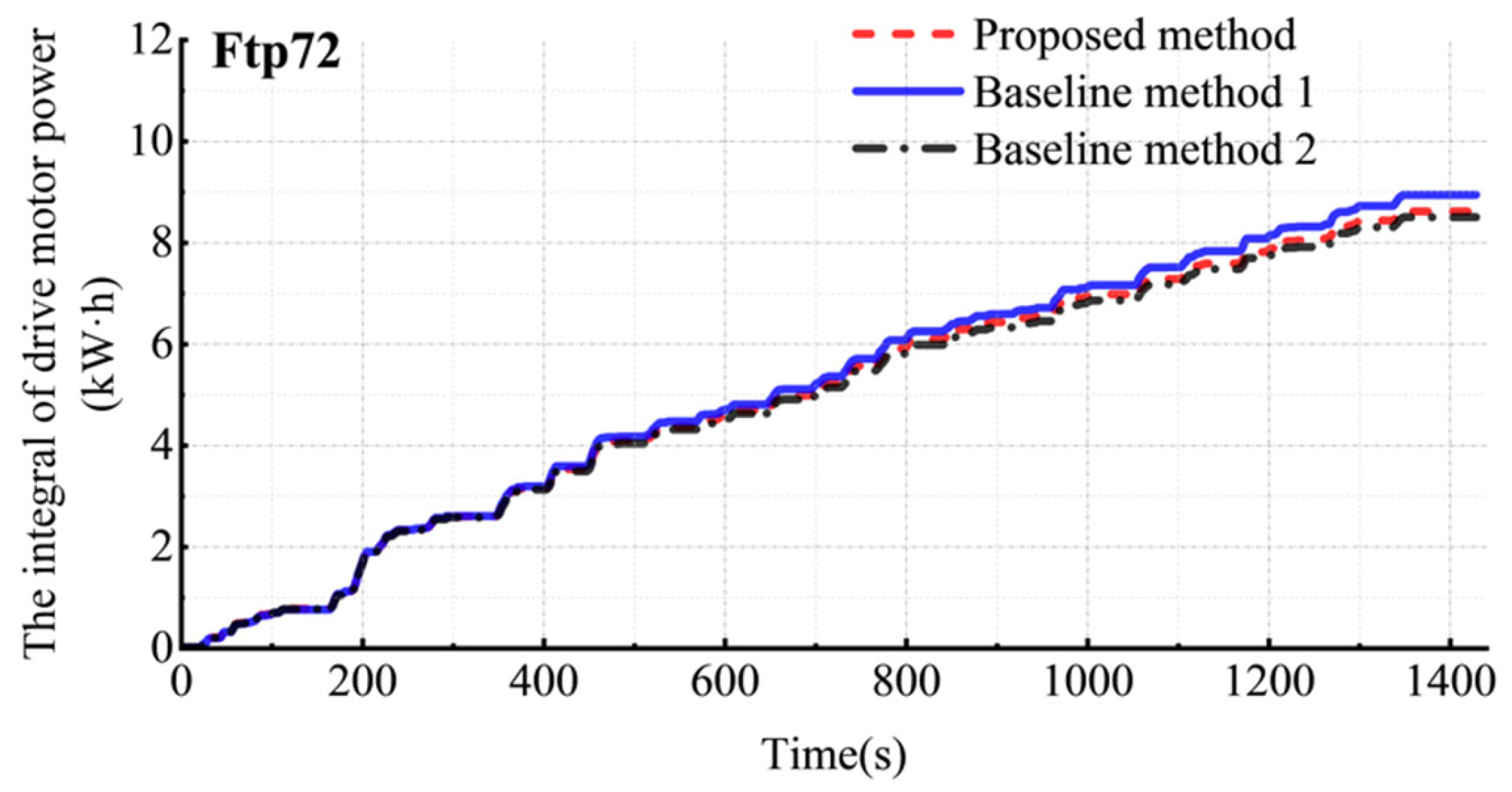
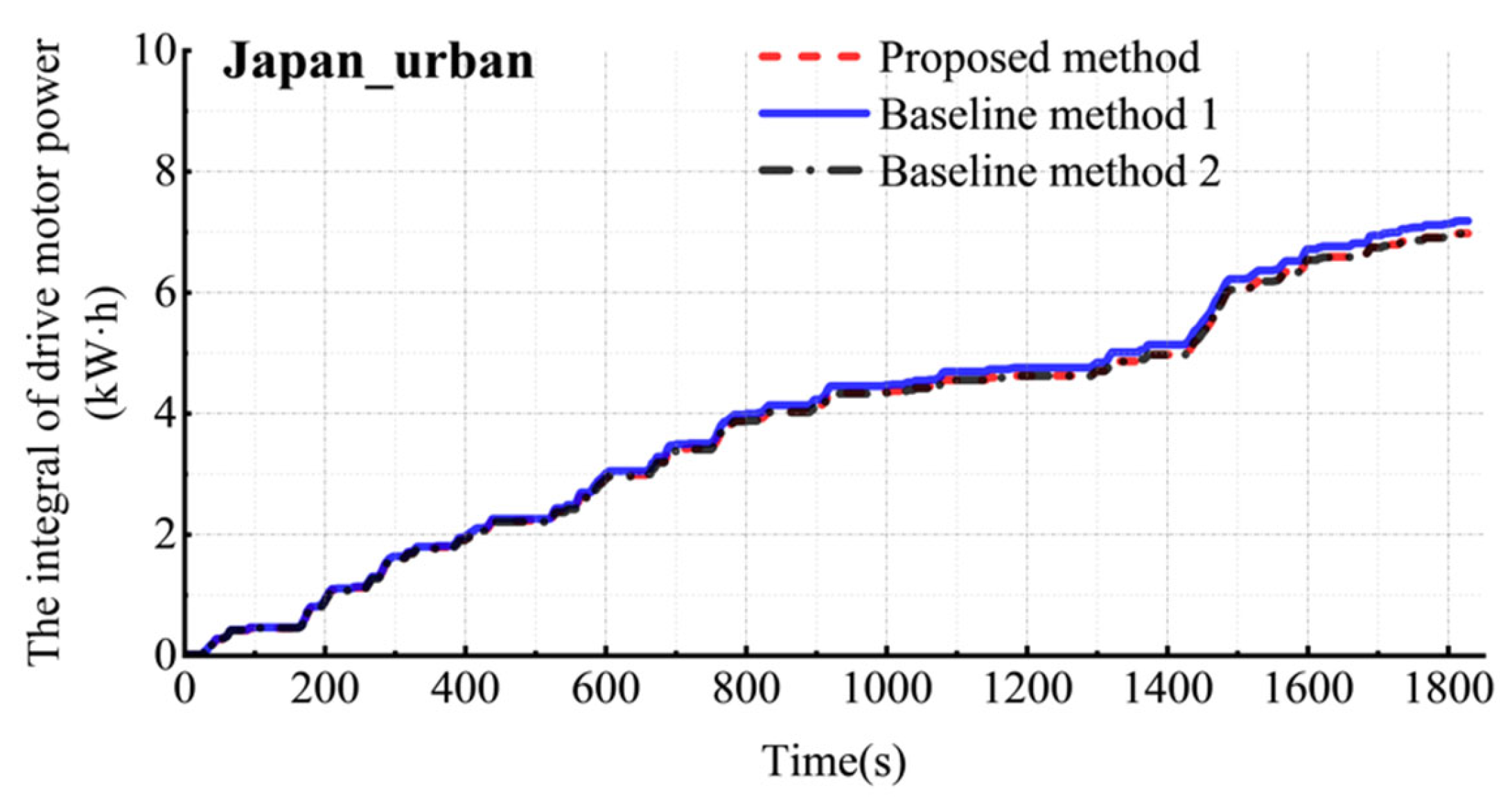
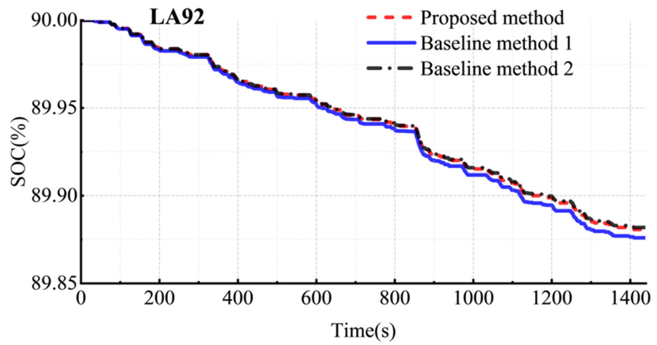
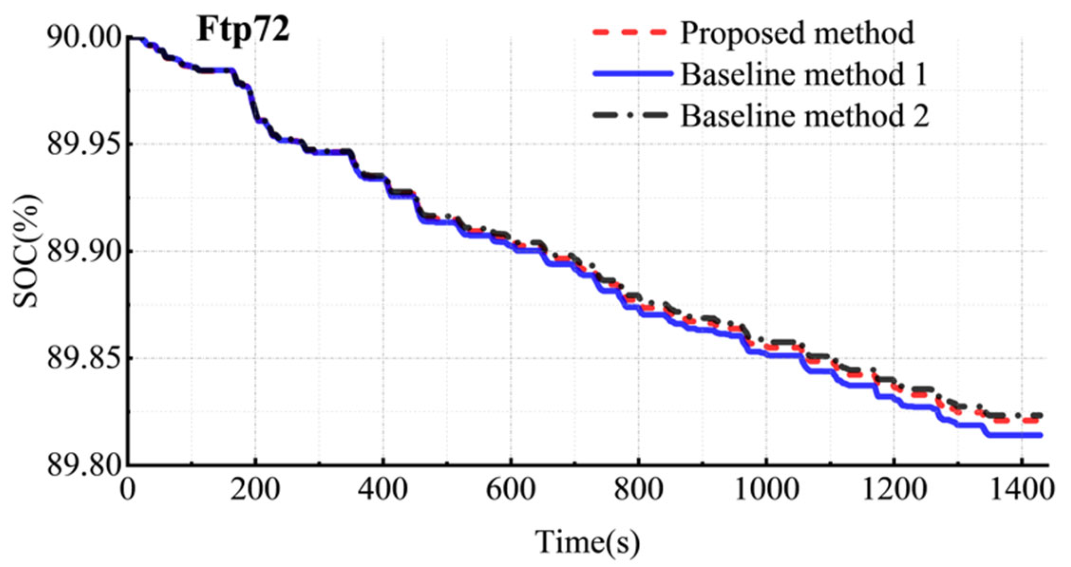
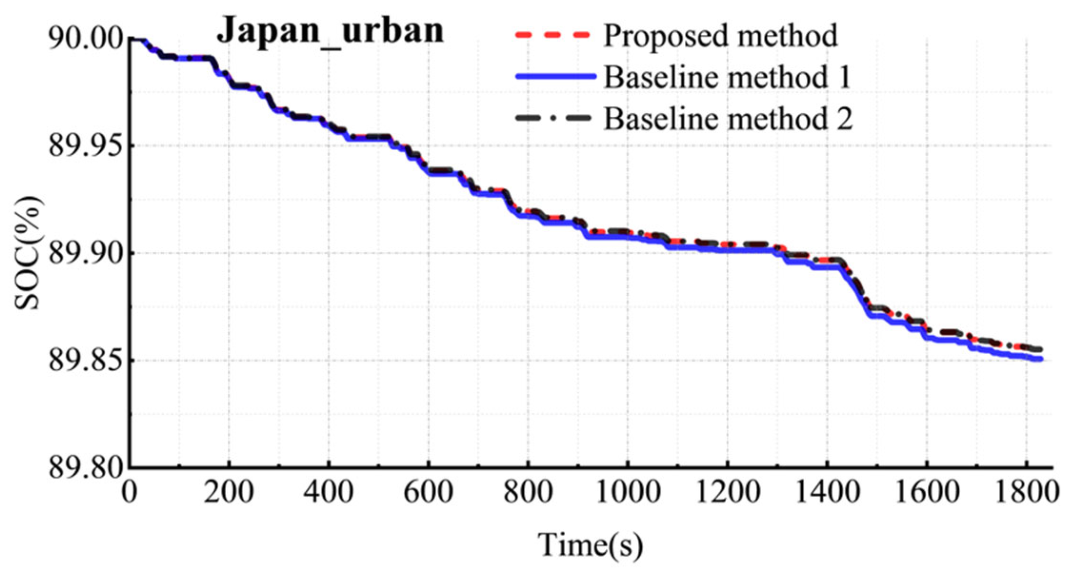
To enhance the reliability of the simulation data, the economic comparison results under the LA92, Ftp72, and Japan_urban driving cycles were studied successively. The power comparison diagrams of the drive motors are shown in Figure 22, Figure 23 and Figure 24, and the SOC characteristic comparison diagrams are shown in Figure 25, Figure 26 and Figure 27.

Table 6. Drive motor power comparison.

	Proposed Method	Baseline Method 1	Baseline Method 2	Units
LA92	5.73	5.97	5.68	kW·h
Ftp72	8.61	8.94	8.50	kW·h
Japan_urban	6.97	7.18	6.96	kW·h

shows the drive motor power comparison.

In Figure 22, the drive motor power of baseline method 1 is 5.97 kW·h, while that of the proposed method under the same driving cycle is 5.73 kW·h. The optimized shift control strategy thus proves to be more economical. The data show that, compared with the vehicle-speed-based shift strategy, the optimized shift control strategy reduces the drive motor power by 4.02%. In Figure 23, the drive motor power of the Ftp72 control group is 8.94 kW·h, while that of the Ftp72 experimental group under the same driving cycle is 8.61 kW·h. The optimized shift control strategy reduces the drive motor power by 3.69%. In Figure 24, the drive motor power of the Japan_urban control group is 7.18 kW·h, while that of the Japan_urban experimental group under the same driving cycle is 6.97 kW·h. The optimized shift control strategy reduces the drive motor power by 2.92%.

Compared with baseline method 2, the proposed method increases the energy consumption by 0.88%, 1.29%, and 0.14% in the LA92, Ftp72, and Japan_urban cycles, respectively.

The SOC is 90% in Figure 25. The remaining SOC of the LA92 control group is 89.8756%, while that of the LA92 experimental group is 89.8805%. After applying the optimized shift control strategy, the remaining SOC increases by 0.0049 percentage points, while the energy consumption of the LA92 control group is 0.1244%. The driving range increases by 3.94% under the optimized shift control strategy compared to the baseline method. In Figure 26, with an initial SOC of 90%, the remaining SOC of the Ftp72 control group is 89.8137%, while that of the Ftp72 experimental group is 89.8206%. After applying the optimized shift control strategy, the remaining SOC increases by 0.0069 percentage points, the energy consumption of the Ftp72 control group is 0.1863%, and the driving range is improved by 3.7%. In Figure 27, with an initial SOC of 90%, the remaining SOC of the Japan_urban control group is 89.8504%, and that of the Japan_urban experimental group is 89.8548%. After optimizing the shift control strategy, the remaining SOC increases by 0.0044 percentage points. In the Japan_urban driving cycle, the control group consumes 0.1496% of energy, and the driving range is increased by 2.94%.

Table 7. Comparison of SOC changes.

	Proposed Method	Baseline Method 1	Baseline Method 2	Units
LA92	0.1195	0.1244	0.1184	%
Ftp72	0.1794	0.1863	0.1770	%
Japan_urban	0.1452	0.1496	0.1451	%

shows the comparison of SOC changes.

Under the LA92, Ftp72, and Japan_urban driving cycles, compared with the conventional vehicle-speed-based shift control strategy, the optimized strategy reduces the drive motor power by 4.02%, 3.69%, and 2.92%, respectively, and increases the driving range by 3.94%, 3.7%, and 2.94%, respectively. In Figure 25, Figure 26 and Figure 27, the remaining SOC of the proposed method increases by 0.93%, 1.36%, and 0.07% compared to baseline method 2 in the LA92, Ftp72, and Japan_urban cycles, respectively. The two methods exhibit comparable performance in terms of improving economic efficiency.

4.1.5. Smoothness Comparison

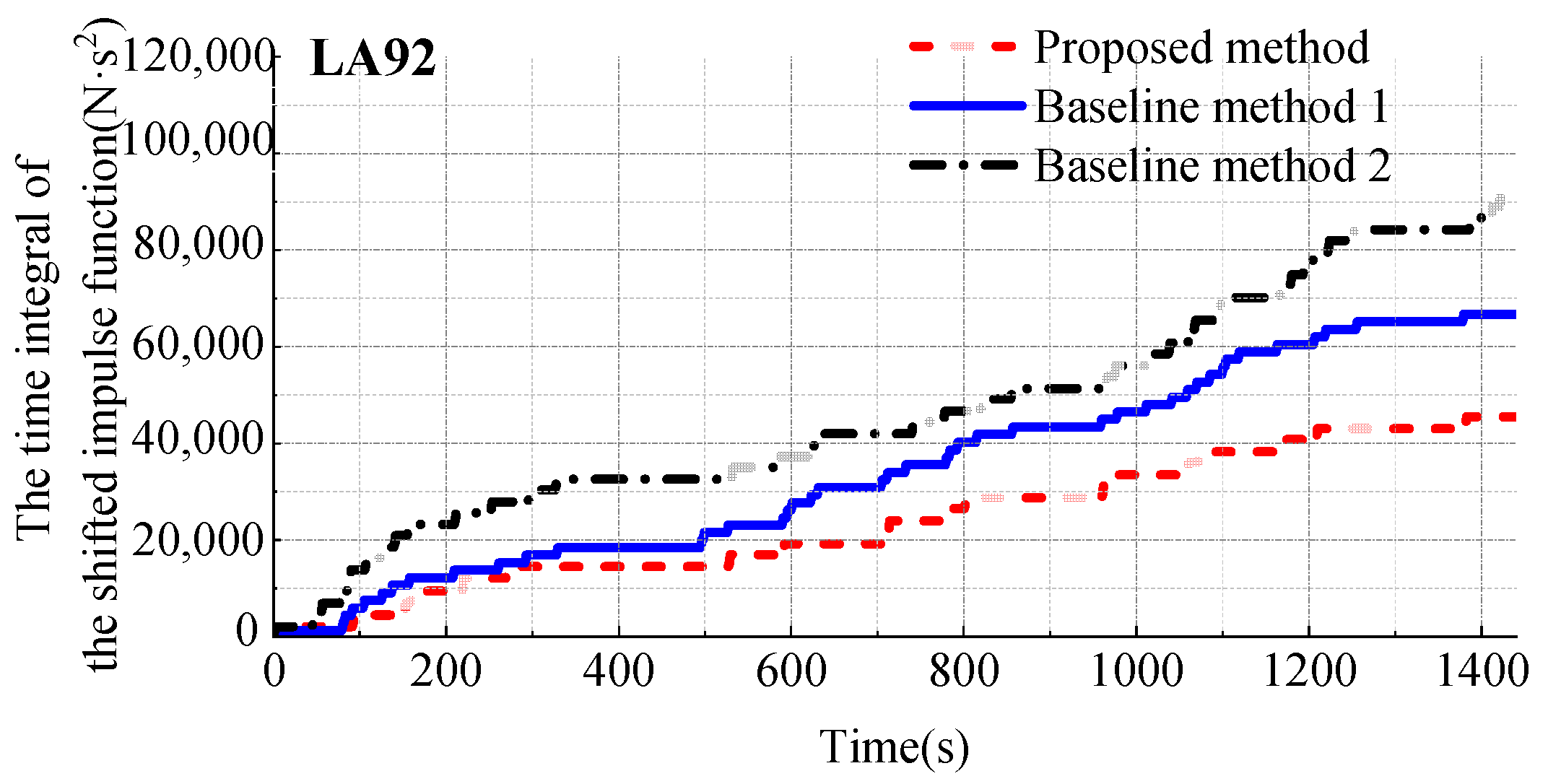
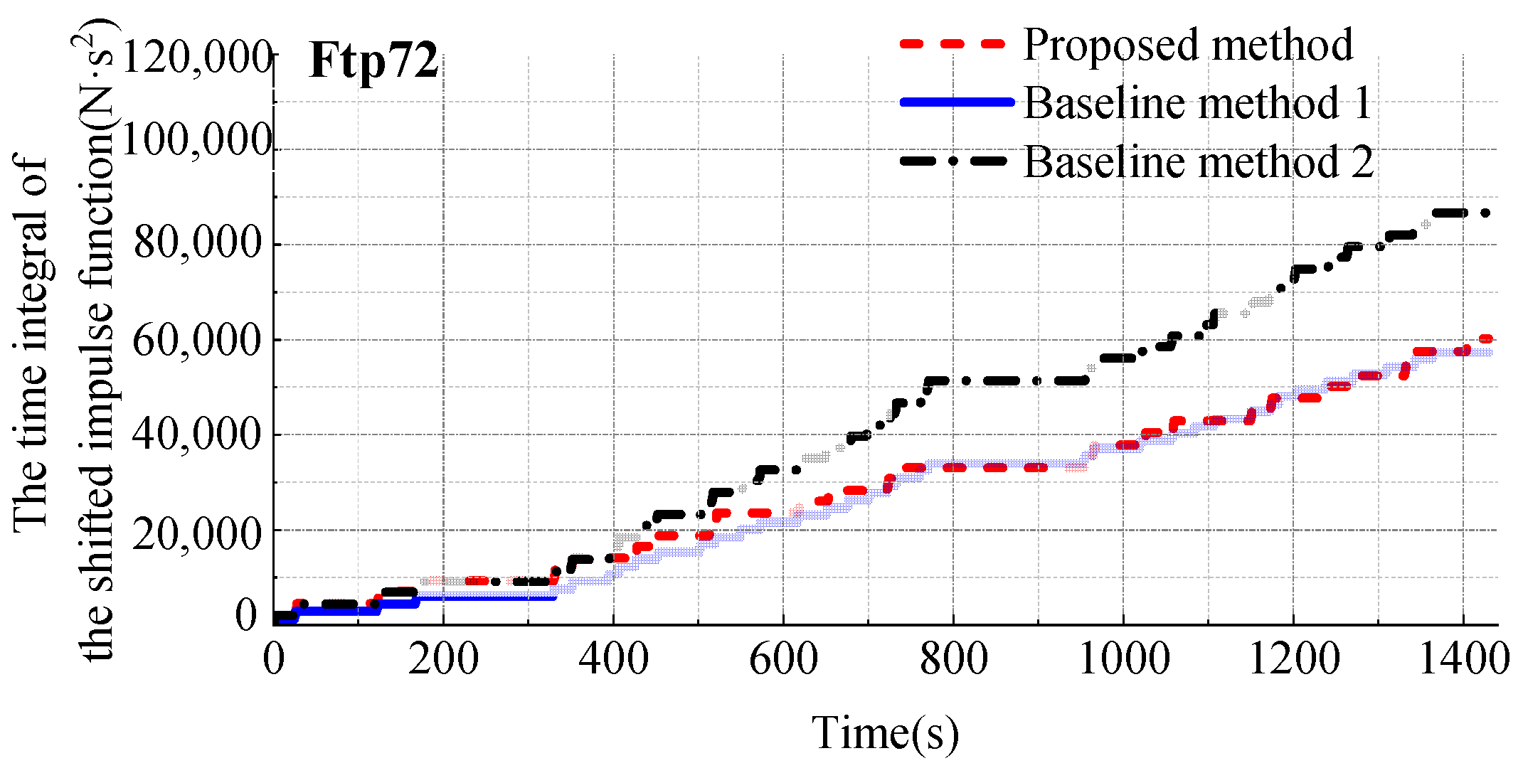
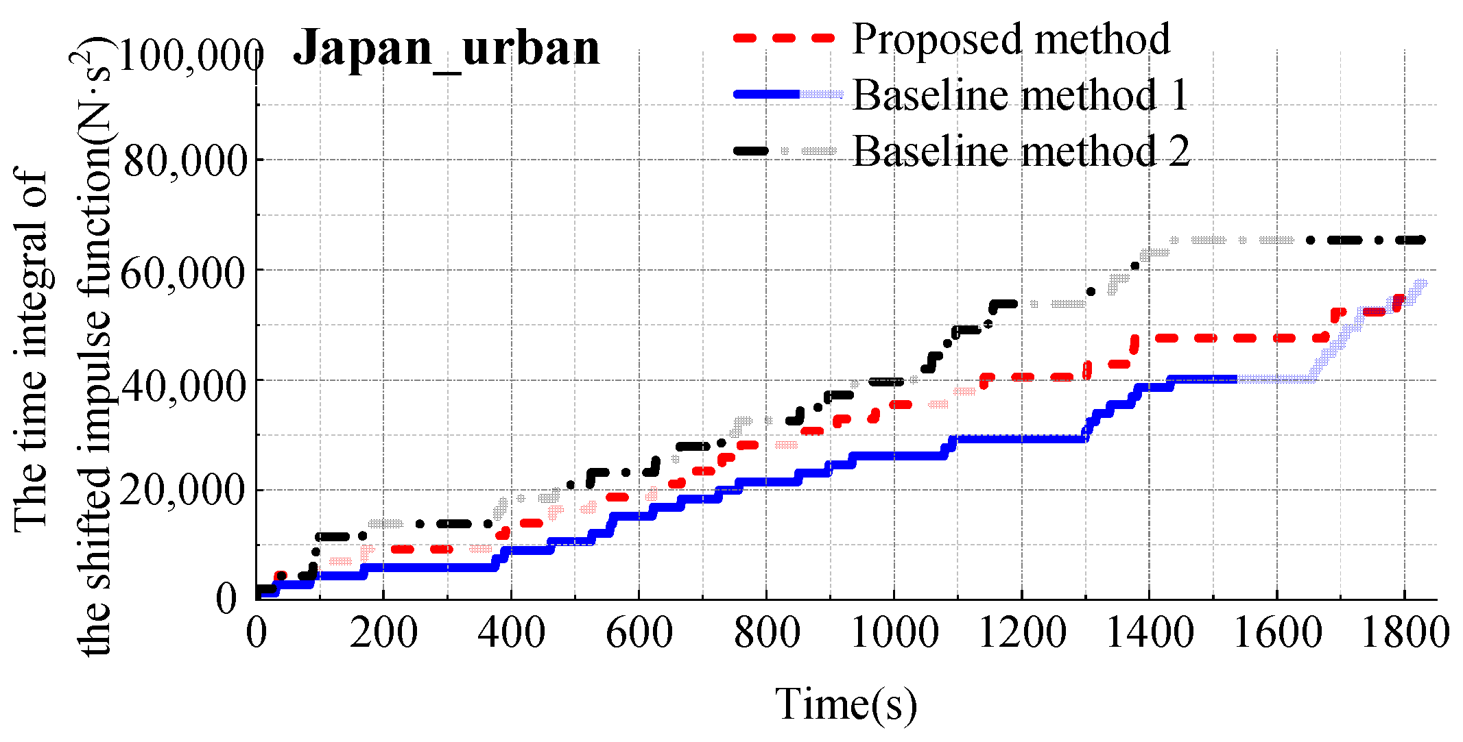
The integral of the shift impulse over time is adopted as the quantitative index of power shock. Based on the LA92, Ftp72, and Japan_urban driving cycles, a comparative analysis was conducted on the smoothness of the proposed method, baseline method 1, and baseline method 2. Figure 28, Figure 29 and Figure 30 present schematic diagrams of the dynamic impact comparison.

Table 8. Smoothness comparison results.

	Proposed Method	Baseline Method 1	Baseline Method 2	Units
LA92	45,475	66,687	91,351	N·s2
Ftp72	57,499	57,346	86,667	N·s2
Japan_urban	54,858	57,517	67,865	N·s2

shows the smoothness comparison.

The smoothness index values of the proposed method, baseline method 1, and baseline method 2 are 45,475, 66,687, and 91,351 N·s² in the LA92 driving cycle. Relative to baseline method 1, the smoothness index of the proposed method is improved by 31.81%; relative to baseline method 2, it is reduced by 50.22%. In the Ftp72 driving cycle, the smoothness index values of the proposed method, baseline method 1, and baseline method 2 are 57,499, 57,346, and 86,667 N·s². The proposed method shows a 0.26% increase in smoothness index compared with baseline method 1, and a 33.66% decrease compared with baseline method 2. In the Japan_urban driving cycle, the smoothness index values of the proposed method, baseline method 1, and baseline method 2 are 54,858, 57,517, and 67,865 N·s². The smoothness of the proposed method is 4.62% lower than that of baseline method 1, indicating a slightly improved comfort level. The smoothness of the proposed method is 19.17% lower than that of baseline method 2.

From the above comparison and analysis of power shock, it is found that the smoothness is improved by 31.81% in the LA92 driving cycle and by 4.62% in the Japan_urban driving cycle compared to baseline method 1. The smoothness is essentially unchanged compared to baseline method 1 in the Ftp72 driving cycle. It is found that the smoothness is improved by 50.22%, 33.66%, and 19.17% compared to baseline method 2 in the LA92, Ftp72, and Japan_urban driving cycles, respectively.

4.2. HIL: Shifting Motor Test

Bench testing, as a core technical means for the development and verification of vehicle power systems, plays an irreplaceable role in the optimization and verification of shift strategies. Through systematic testing in a high-precision and controllable environment, it can accurately quantify the impact of shift strategies on power performance, economy, ride comfort, and durability, providing data support for the correction of theoretical models and the iteration of control algorithms.

Due to insufficient test conditions, this paper completed the functional test of the shift motor based on the PC end, tested the sensitivity of the shift motor, calculated the error between the actual speed of the shift motor and the required speed, and verified the feasibility of optimizing the shift execution process by controlling the speed of the shift motor.

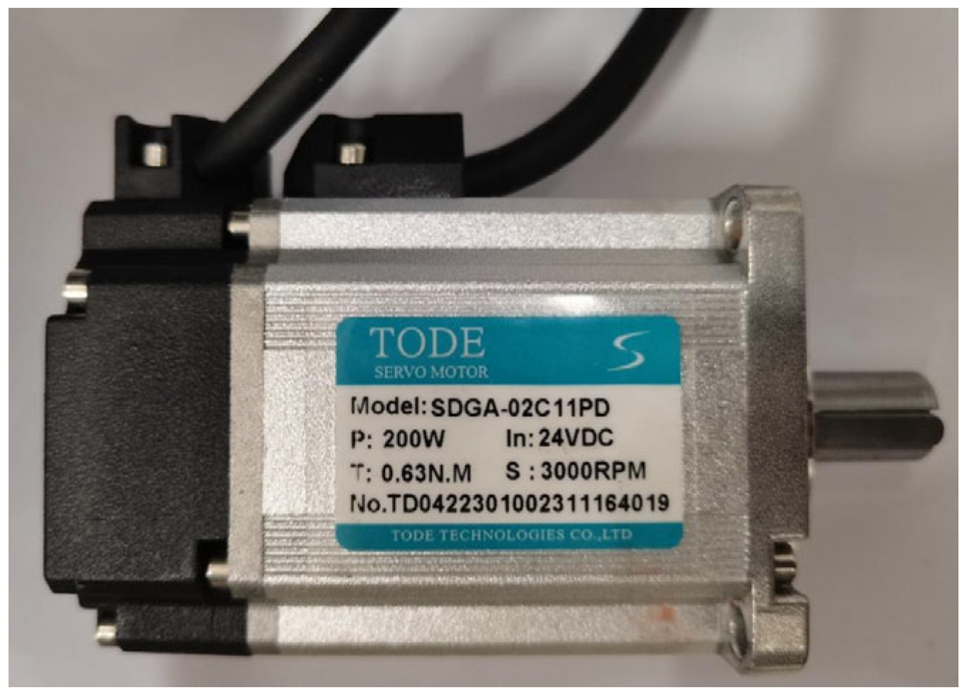
To design the functional test of the shift motor for the two-speed AMT of electric vehicles, the core lies in controlling the driver through the upper computer on the PC end, thereby controlling the speed and rotation direction of the shift motor to simulate the real shift situation. The test consists of a shifting motor, a driver, and a PC-end control platform. The selection of test components is an indispensable step in the test process. First, the selection of the host computer was carried out. In this paper, TODE-MotorHost was selected as the test host computer. Second, the selection of the gear shifting motor was completed. The selected motor is a 200 W/24 VDC permanent magnet synchronous motor with a rated speed of 3000 RPM, as shown in Figure 31. Thirdly, the selection of the driver was made, and the TODE driver that matches the permanent magnet synchronous motor was chosen. Fourth, the communication signal was selected, and CAN communication was chosen.

Functional testing, as the primary step in verifying the fundamental performance and reliability of the power transmission system, plays a foundational role throughout the entire testing process. Through systematic no-load operation, static shifting, and fault injection tests, it ensures that each subsystem of the transmission (such as shift actuators, synchronizers, sensors, and control systems) meets design specifications and functional safety requirements in a controlled environment, laying the foundation for subsequent performance testing and durability assessment.

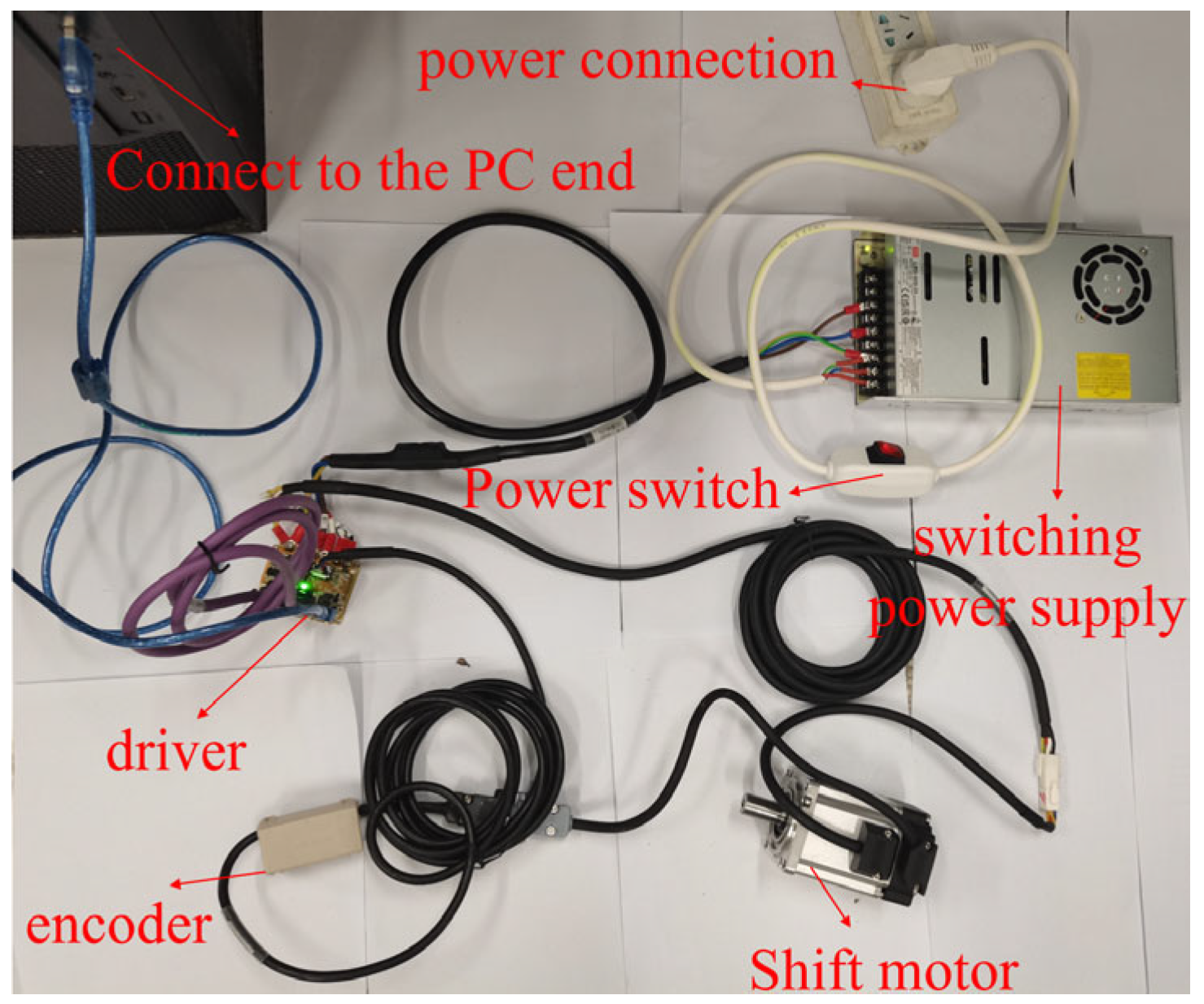
The function test of the shift motor aims to verify whether the shift motor can operate according to the data controlled by the PC in the shift motor test, and whether its functionality is good. Figure 32 presents the wiring diagram of the shift motor. To complete the functional test of the shift motor, a test bench needs to be set up. The assembly and wiring of the stand and the PC end require the installation of a switching power supply and a three-hole plug with a switch. First, the shift motor is wired to the driver; then, the drive motor is connected to the computer host. Next, the wiring of the switching power supply and the driver is completed, and then the three-hole plug is connected via the switch to the switching power supply. Finally, the three-hole power plug is connected via the switch to the power socket to complete the power-on process.

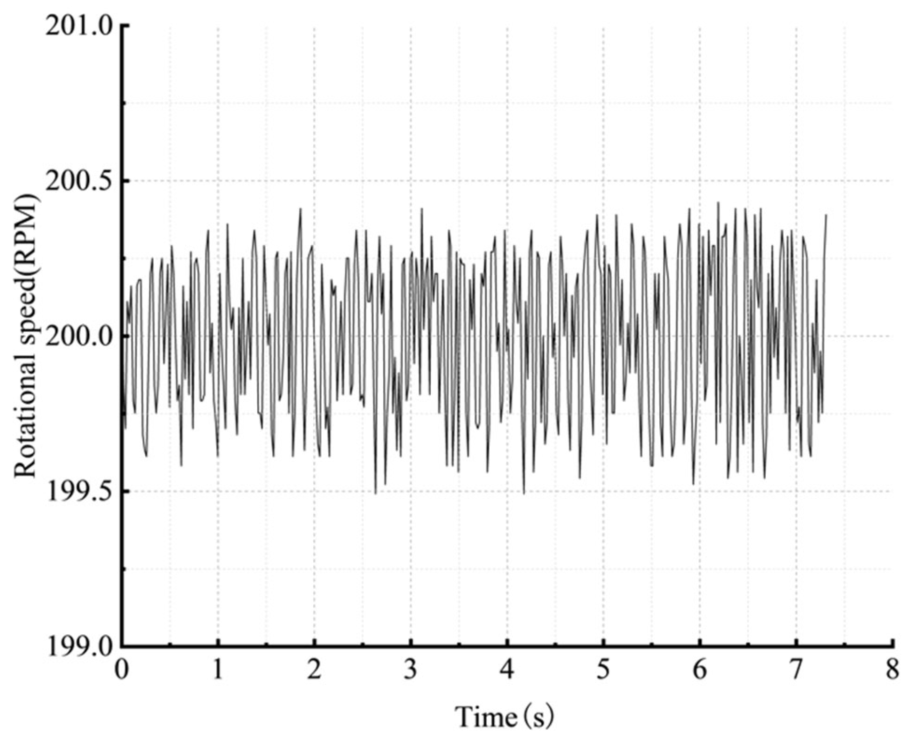
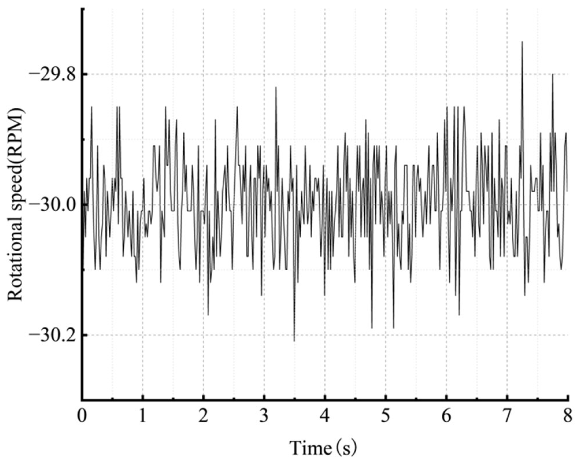
After the wiring is completed, PC control is performed. The shift control strategy designed in this paper optimizes the shift execution process by controlling the rotational speed of the shift motor. The target rotational speed of the shift motor is input on the PC end to test the functionality of the shift motor. The specified speed is 200 RPM, which is input to the PC end. The speed of the shifting motor fluctuates normally, with a fluctuation amplitude of 0.51 RPM and an error of less than 1%. The average rotational speed is 200.00 RPM, and the error is negligible. Figure 33 shows the actual rotational speed of the shifting motor at the target 200 RPM. The specified speed is −30 RPM, that is, the reverse rotation speed is 30 RPM. The speed of the shifting motor fluctuates normally, with a fluctuation amplitude of 0.25 RPM and an error of less than 1%. The average rotational speed is 30.00 RPM, and the error is negligible. Figure 34 shows the actual speed of the shifting motor at the target −30 RPM.

During the above process, the error is less than 1%, meaning that the gear shifting motor operates at the input speed on the PC end, demonstrating good functionality. The feasibility of optimizing the shift execution process by controlling the speed of the shift motor in this paper is high.

5. Discussion

The research object of this paper is the two-speed AMT of heavy-duty electric military armored vehicles. The main research content is the shift control strategy of the two-speed AMT of electric heavy-duty vehicles, considering the driver’s driving style and real-time prediction of driving cycles. Aiming at the problem that the shift speed and timing of the two-speed AMT of electric heavy-duty vehicles do not meet the driver’s requirements and shift frequently, a two-speed AMT shift control model, including the drive motor, power battery, etc., was built, and a fuzzy PID electric vehicle shift control strategy, based on driving style and driving condition prediction, was proposed. The operation rules of the shift control strategy under various driving cycles of the vehicle were analyzed, effectively improving the vehicle’s power characteristics, economy, and driving smoothness.

The gear shifting motor test was completed. The results show that the motor operates according to the data input on the PC end and has good functionality. The feasibility of optimizing the shift execution process by controlling the speed of the shift motor in this paper is high.

Although this shift control strategy effectively met the driver’s expectations, there are still some shortcomings:

(1)

The research results rely mainly on simulation. The applicability of the proposed strategy under actual operating conditions remains unverified. Real roads feature varying gradients, which differ from the simulation environment.

(2)

Regarding the structural design and dynamic analysis of the two-speed AMT for electric vehicles, the dynamic model designed in this paper is relatively simplified, ignoring the energy loss caused by partial heat dissipation in the transmission system and the changes in the air density and air resistance coefficient during vehicle operation.

(3)

In terms of the research on the two-speed AMT control strategy for electric vehicles, when calculating the condition prediction matrix based on the Markov chain model in this paper, only 10 sets of driving cycles were sampled, and the predicted speed of the next 2 s was found to be a little off based on the actual speed.

6. Conclusions

This article proposes a shift control strategy based on vehicle speed prediction and driving style recognition for AMT by optimizing the shifting strategy to meet the driver’s driving needs. The driving style recognition model based on impact degree and a condition prediction model based on the Markov chain model were designed, and the driving style and predicted vehicle speed were introduced to optimize the gear shifting decision-making process. The fuzzy controller with driving style and predicted vehicle speed as inputs and a gear adaptive model to avoid frequent gear shifting were designed. The target gear was adjusted to optimize the gear shifting decision-making process for the second time. The simulation and test results show that the proposed approach effectively improves the vehicle’s power characteristics, economy, and driving smoothness compared to the conventional strategy. Compared with the adaptive shift schedule design method of [14], the proposed approach reduces shift frequency and improves ride comfort by at least 19.17% under similar dynamic performance and fuel economy conditions.

Future work will focus on the validation of the proposed strategy under varying loads, road slopes, and other real-world factors. To further optimize the shifting strategy, the following research directions will be pursued. First, additional driving cycles will be sampled to reduce the prediction error for vehicle speed over the next two seconds. Second, a joint simulation platform integrating CarSim and MATLAB/Simulink will be established to conduct a higher-quality simulation analysis. Third, real vehicle tests will be conducted to enhance test data reliability.

References

1. Rejeb, A.; Rejeb, K.; Süle, E.; Lahbib, M.; Simske, S. A Review of Two Decades of Academic Research on Electric Vehicle Battery Supply Chains: A Bibliometric Approach. Vehicles 2026, 8, 1. [Google Scholar]
2. Teodorascu, V.; Burnete, N.; Kocsis, L.B.; Duma, I.; Burnete, N.V.; Molea, A.; Sechel, I.C. Development of the Electrical Assistance System for a Modular Attachment Demonstrator Integrated in Lightweight Cycles Used for Urban Parcel Transportation. Vehicles 2025, 7, 164. [Google Scholar] [CrossRef]
3. Comi, A.; Crisalli, U.; Hriekova, O.; Idone, I. Analysis of the Willingness to Shift to Electric Vehicles: Critical Factors and Perspectives. Vehicles 2025, 7, 159. [Google Scholar] [CrossRef]
4. He, Y.; Sui, S.; Wang, Q.; Jin, Y.; Zhang, L. Super-high speed AMT shifting strategy and energy consumption optimization for electric vehicle. Energy 2025, 322, 135489. [Google Scholar] [CrossRef]
5. De Pinto, S.; Camocardi, P.; Sorniotti, A.; Gruber, P.; Perlo, P.; Viotto, F. Torque-Fill Control and Energy Management for a Four-Wheel-Drive Electric Vehicle Layout with Two-Speed Transmissions. IEEE Trans. Ind. Appl. 2017, 53, 447–458. [Google Scholar]
6. Wu, J.; Zhang, N. Driving mode shift control for planetary gear based dual motor powertrain in electric vehicles. Mech. Mach. Theory 2021, 158, 104217. [Google Scholar] [CrossRef]
7. Ivan, C.; Joško, D.; Mislav, H.; Zhang, Y.; Vladimir, I. Static Model-Based Optimization and Multi-Input Optimal Control of Automatic Transmission Upshift during Inertia Phase. Vehicles 2023, 5, 177–202. [Google Scholar]
8. Ranogajec, V.; Deur, J.; Ivanović, V.; Tseng, H.E. Multi-objective Parameter Optimization of Control Profiles for Automatic Transmission Double-Transition Shifts. Control Eng. Pract. 2019, 93, 104183. [Google Scholar]
9. Kihan, K.; Junhyeong, J.; Seungjae, M. Multi-Objective Gear Ratio and Shifting Pattern Optimization of Multi-Speed Transmissions for Electric Vehicles Considering Variable Transmission Efficiency. Energy 2021, 236, 121419. [Google Scholar]
10. Liu, H.; Yang, K.; Sun, W.; Liu, L.; Su, Z.; Xiao, Q.; Wang, S.; Li, S. Research on Energy Management Strategy for Range-Extended Electric Vehicles Based on Eco-Driving Speed. Appl. Sci. 2025, 15, 12738. [Google Scholar]
11. Xi, J.; Si, H.; Gao, J. Optimization of a Shift Control Strategy for Pure Electric Commercial Vehicles Based on Driving Intention. World Electr. Veh. J. 2024, 15, 44. [Google Scholar] [CrossRef]
12. Chen, Z.; Xiong, R.; Wang, C.; Cao, J. An On-Line Predictive Energy Management Strategy for Plug-in Hybrid Electric Vehicles to Counter the Uncertain Prediction of the Driving Cycle. Appl. Energy 2017, 185, 1663–1672. [Google Scholar]
13. Kang, M.; Gao, J. Design of an Eco-Gearshift Control Strategy under a Logic System Framework. Front. Inf. Technol. Electron. Eng. 2020, 21, 340–350. [Google Scholar] [CrossRef]
14. Liu, X.; Du, J.; Cheng, X.; Zhu, Y.; Ma, J. An Adaptive Shift Schedule Design Method for Multi-Gear AMT Electric Vehicles Based on Dynamic Programming and Fuzzy Logical Control. Machines 2023, 11, 915. [Google Scholar] [CrossRef]
15. Yang, C.; Jiao, X.; Li, L.; Zhang, Y.; Zhang, L.; Song, J. Robust Coordinated Control for Hybrid Electric Bus with Single-Shaft Parallel Hybrid Powertrain. IET Control Theory Appl. 2015, 9, 270–282. [Google Scholar]
16. Li, L.; Zhao, X.; Xiong, R.; He, H. AMT Downshifting Strategy Design of HEV During Regenerative Braking Process for Energy Conservation. Appl. Energy 2016, 183, 914–925. [Google Scholar] [CrossRef]
17. Jo, C.; Ko, J.; Yeo, H.; Kim, H.; Lee, K.; Yi, K. Cooperative Regenerative Braking Control Algorithm for an Automatic-Transmission-Based Hybrid Electric Vehicle During a Downshift. Proc. Inst. Mech. Eng. Part D J. Automob. Eng. 2012, 226, 457–467. [Google Scholar]
18. Zhang, S.; Xiong, R.; Cao, J. Battery Durability and Longevity Based Power Management for Plug-in Hybrid Electric Vehicle with Hybrid Energy Storage System. Appl. Energy 2016, 179, 316–328. [Google Scholar] [CrossRef]
19. Li, L.; You, S.; Yang, C.; Yan, B.; Song, J.; Chen, Z. Driving-Behavior-Aware Stochastic Model Predictive Control for Plug-in Hybrid Electric Buses. Appl. Energy 2016, 162, 868–897. [Google Scholar]
20. Du, J.; Zhang, X.; Wang, S.; Liu, X.; Xing, M. A Novel ANFIS-Dynamic Programming Fusion Strategy for Real-Time Energy Management Optimization in Fuel Cell Electric Commercial Vehicles. Electronics 2025, 14, 4601. [Google Scholar]
21. Wang, S.; Zhang, H.; Zhao, X.; Zheng, Z.; Song, H. Research on Lateral Stability Control Strategy for Distributed Drive Electric Vehicles Considering Driving Style. J. Frankl. Inst. 2024, 361, 106921. [Google Scholar] [CrossRef]
22. RayniNejad, H.M.; Keynia, F.; Ahmadinia, M.; Molahosseini, A.S. A new state of charge prediction method for electric vehicles by an attention-based SAE-BiLSTM model: Analyzing driving styles and vehicle types with operational and environmental data. J. Energy Storage 2025, 133, 118049. [Google Scholar]
23. Lin, X.; Li, Y.; Xia, B. An online driver behavior adaptive shift strategy for two-speed AMT electric vehicle based on dynamic corrected factor. Sustain. Energy Technol. Assess. 2021, 48, 101598. [Google Scholar] [CrossRef]
24. Fu, Z.; Li, M.; Tao, F.; Zhu, L.; Wang, J. Predictive energy management strategy based on driving behavior identification for fuel cell hybrid electric vehicle in car-following scenario. Int. J. Hydrogen Energy 2025, 176, 151486. [Google Scholar] [CrossRef]
25. Jawad, Y.K.; Nitulescu, M. Improving Driving Style in Connected Vehicles via Predicting Road Surface, Traffic, and Driving Style. Appl. Sci. 2024, 14, 3905. [Google Scholar] [CrossRef]
26. Liu, G.; Guo, F.; Liu, Y.; Zhang, Y.; Liu, Y. Weighted Double Q-Learning Based Eco-Driving Control for Intelligent Connected Plug-in Hybrid Electric Vehicle Platoon with Incorporation of Driving Style Recognition. J. Energy Storage 2024, 86, 111282. [Google Scholar]
27. Yuan, W.; Han, Y.; Lu, Y.; Zhang, Y.; Ge, Y. Prediction of driving energy consumption for pure electric buses using dynamic driving style recognition and speed forecasting. Energy 2025, 329, 136785. [Google Scholar] [CrossRef]
28. Shin, J.; Sunwoo, M. Vehicle Speed Prediction Using a Markov Chain with Speed Constraints. IEEE Trans. Intell. Transp. Syst. 2019, 20, 3201–3211. [Google Scholar]
29. Liu, H.; Li, X.; Wang, W.; Han, L.; Xiang, C. Markov velocity predictor and radial basis function neural network-based real-time energy management strategy for plug-in hybrid electric vehicles. Energy 2018, 152, 427–444. [Google Scholar]
30. Silva, F.L.; Eckert, J.J.; Miranda, M.H.; da Silva, S.F.; Silva, L.C.; Dedini, F.G. A Comparative Analysis of Optimized Gear Shifting Controls for Minimizing Fuel Consumption and Engine Emissions Using Neural Networks, Fuzzy Logic, and Rule-Based Approaches. Eng. Appl. Artif. Intell. 2024, 135, 108777. [Google Scholar] [CrossRef]
31. Ahmed, M.U.; Qays, M.O.; Lachowicz, S.; Mahmud, P. Optimizing EV Battery Charging Using Fuzzy Logic in the Presence of Uncertainties and Unknown Parameters. Electronics 2026, 15, 177. [Google Scholar]
Figure 1. The transmission system.
Vehicles 08 00157 g001
Figure 2. Longitudinal dynamic analysis of the vehicle.
Vehicles 08 00157 g002
Figure 3. Shift control strategy.
Vehicles 08 00157 g003
Figure 4. Flowchart of driving style recognition based on impact degree.
Vehicles 08 00157 g004
Figure 5. Vehicle speed prediction.
Vehicles 08 00157 g005
Figure 6. Probability output matrix of the Markov chain model: (a) step 1; (b) step 2; (c) step 3; and (d) step 4.
Vehicles 08 00157 g006
Figure 7. Fuzzy control process.
Vehicles 08 00157 g007
Figure 8. Fuzzy rule 1.
Vehicles 08 00157 g008
Figure 9. Adaptive adjustment flowchart.
Vehicles 08 00157 g009
Figure 10. Fuzzy rule curve graph: (a) Fuzzy rule input curve of the rate of change in rotational speed difference; (b) input curve of fuzzy rules for speed difference; and (c) output curve of the fuzzy rule for the speed demand coefficient of the shift motor.
Vehicles 08 00157 g010
Figure 11. PID controller.
Vehicles 08 00157 g011
Figure 12. Fuzzy PID control system.
Vehicles 08 00157 g012
Figure 13. LA92 driving cycle and predicted vehicle speed.
Vehicles 08 00157 g013
Figure 14. Ftp72 driving cycle and predicted vehicle speed.
Vehicles 08 00157 g014
Figure 15. Japan_urban driving cycle and predicted vehicle speed.
Vehicles 08 00157 g015
Figure 16. Comparison of vehicle gears in the LA92 driving cycle.
Vehicles 08 00157 g016
Figure 17. Comparison of vehicle gears in the Ftp72 driving cycle.
Vehicles 08 00157 g017
Figure 18. Comparison of vehicle gears in the Japan_urban driving cycle.
Vehicles 08 00157 g018
Figure 19. Dynamic performance comparison in the LA92 driving cycle.
Vehicles 08 00157 g019
Figure 20. Dynamic performance comparison in the Ftp72 driving cycle.
Vehicles 08 00157 g020
Figure 21. Dynamic performance comparison in Japan_urban driving cycle.
Vehicles 08 00157 g021
Figure 22. Comparison chart of the drive motor power in the LA92 driving cycle.
Vehicles 08 00157 g022
Figure 23. Comparison chart of the drive motor power in the Ftp72 driving cycle.
Vehicles 08 00157 g023
Figure 24. Comparison chart of the drive motor power in the Japan_urban driving cycle.
Vehicles 08 00157 g024
Figure 25. Comparison of SOC characteristics in the LA92 driving cycle.
Vehicles 08 00157 g025
Figure 26. Comparison of SOC characteristics in the Ftp72 driving cycle.
Vehicles 08 00157 g026
Figure 27. Comparison chart of SOC characteristics in the Japan_urban driving cycle.
Vehicles 08 00157 g027
Figure 28. Comparison chart of shift impulse and time in the LA92 driving cycle.
Vehicles 08 00157 g028
Figure 29. Comparison chart of shift impulse and time in the Ftp72 driving cycle.
Vehicles 08 00157 g029
Figure 30. Comparison chart of shift impulse and time in the Japan_urban driving cycle.
Vehicles 08 00157 g030
Figure 31. Shift motor.
Vehicles 08 00157 g031
Figure 32. HIL testing.
Vehicles 08 00157 g032
Figure 33. Actual rotational speed of the shifting motor at the target 200 RPM.
Vehicles 08 00157 g033
Figure 34. Actual rotational speed of the shifting motor at the target −30 RPM.
Vehicles 08 00157 g034