Real-Time Tire–Road Friction Coefficient Estimation for Four-Wheel-Independent-Drive Electric Vehicles Using a Piecewise Gain-Scheduled Observer and Neural Networks

Abstract

Four-wheel-independent-drive electric vehicles are gaining increasing research attention due to their comprehensive dynamic performance. Real-time tire–road friction coefficient information contributes to the development of adaptive control algorithms and active safety control systems for such vehicles. However, traditional tire models widely adopted in existing estimation methods may fail to match practical tire characteristics accurately. Furthermore, lateral velocity serves as a critical state variable for tire–road friction coefficient estimation, whereas existing lateral velocity observers using low-cost inertial measurement unit sensors suffer from degraded estimation performance under complex driving maneuvers. To address the above challenges, this paper proposes a three-stage friction coefficient estimation framework. Firstly, vehicle lateral velocities are estimated via a piecewise gain-scheduled observer using inertial measurement unit measurements. Secondly, tire slip ratios are calculated based on the observed lateral velocities; meanwhile, the longitudinal, lateral and vertical forces of each tire are reconstructed. Lastly, tire force and slip information under combined slip conditions are acquired, and a multilayer perceptron neural network is established to achieve individual tire–road friction coefficient estimation. The simulation results verify the numerical feasibility and preliminary effectiveness of the proposed estimation method under ideal simulation conditions.

1. Introduction

Thanks to recent advancements in electric vehicle technology, four-wheel-independent-drive (4WID) vehicles are becoming increasingly popular. This type of vehicle provides an effective means of enhancing drivability due to the redundant nature of control inputs and the rapid response of motors [1,2,3]. The handling stability of 4WID vehicles can be significantly improved through four-wheel steering, direct yaw moment control, and slip ratio control [4,5]. For these control systems, accurate knowledge of the tire–road friction coefficient (TRFC) is essential, as the maximum traction and braking capabilities of vehicles are directly determined by real-time TRFC conditions [6,7,8].

Real-time acquisition of TRFC is thus crucial for the stable and safe operation of 4WID vehicles. However, TRFC cannot be directly measured by onboard sensors due to technical limitations and high hardware costs, prompting extensive research on indirect estimation methods. Existing estimation strategies can be broadly classified into two categories: special sensor-based methods [9,10,11] and vehicle dynamics-based estimation approaches [12,13,14]. Considering the inherent drawbacks of dedicated sensors, including poor environmental adaptability, limited reliability, and excessive deployment costs, this study focuses on the low-cost and high-feasibility vehicle dynamics-based estimation scheme. According to the adopted dynamic characteristics, mainstream dynamics-based TRFC estimation methods are divided into three categories: (a) estimation systems based solely on longitudinal vehicle dynamics [15,16,17]; (b) estimation systems relying purely on lateral vehicle dynamics [16,18,19]; (c) integrated estimation systems that fuse both longitudinal and lateral dynamic information [20].

For longitudinal dynamics-based estimation methods, TRFC values are predominantly calculated by analyzing the longitudinal and vertical forces exerted on individual tires [6]. These methods fully exploit the distinct tire mechanical characteristics in linear adhesion and nonlinear sliding regions. Furthermore, Xia et al. proposed a slip-based estimation algorithm combining Lyapunov stability theory and a nonlinear observer to identify the maximum road friction coefficient [21]. Moreover, a real-time maximum TRFC estimation approach was developed based on the inherent correlation between wheel slip ratio and friction variation, which achieves accurate estimation through the collaborative design of tire radius observers, normal force observers, and tractive force estimators [22]. Despite their effectiveness under intense longitudinal excitation, such methods suffer from obvious limitations. In conventional daily driving scenarios, vehicle longitudinal slip remains extremely small and stable, resulting in insufficient dynamic excitation for friction identification, which severely degrades the estimation accuracy and robustness of longitudinal dynamics-based methods. To compensate for this defect, lateral dynamics-based estimation techniques have been widely investigated. Hahn et al. developed a TRFC estimation algorithm dependent on vehicle lateral dynamic responses [23], which integrates an empirical lateral tire force model and adaptive parameter identification strategy for real-time friction coefficient calibration. Nevertheless, empirical tire models rely heavily on fixed structural assumptions and cannot fully describe time-varying tire nonlinear characteristics under extreme driving conditions, inevitably introducing cumulative estimation errors. To further improve estimation performance, data-driven methods have been introduced into friction estimation research. The study in [24] designed a particle swarm optimization-long short-term memory (PSO-LSTM) neural network-based estimator combined with lateral dynamic information to support steering controller design. The model takes yaw rate, longitudinal velocity, sideslip angle, yaw rate gain, and front wheel slip angles as inputs and outputs the real-time TRFC.

Although the above longitudinal or lateral single-dynamic methods can realize basic friction coefficient estimation, most of them fail to adapt to complex combined slip scenarios, where both longitudinal and lateral tire forces exist simultaneously. Under actual driving conditions such as turning, acceleration, and deceleration coupling, tires frequently operate in combined slip states, and single-dimensional dynamic information cannot fully reflect tire friction characteristics, leading to limited estimation generalization ability. Aiming at this problem, several integrated dynamic estimation methods have been proposed. Zareian et al. adopted a multilayer perceptron neural network for TRFC estimation, where the offline training of the network is based on the classic Magic Formula tire model [25]. However, the fixed empirical formula cannot adapt to variable road and tire conditions, resulting in poor generalization performance. An integrated KF method fusing front and rear axle lateral and longitudinal dynamic information was proposed in [12], yet the convergence performance of estimation errors was not fully considered, which may cause unstable estimation results under transient driving conditions. To optimize error convergence and anti-interference ability, a fault-tolerant fusion estimation framework with explicit convergence constraints was designed in [26], which realized reliable estimation under sensor missing measurement conditions via adaptive weight fusion strategies. Nevertheless, most existing integrated methods adopt fixed observer parameters and linearized vehicle models, which lack adaptive adjustment capabilities for highly nonlinear and time-varying vehicle operating conditions. In addition, accurate vehicle state acquisition, especially lateral velocity, is the core prerequisite for high-precision friction estimation, while few studies have optimized state observers for complex variable working conditions, restricting the further improvement of friction estimation accuracy.

Furthermore, critical vehicle state parameters, including lateral velocity, slip ratio, and sideslip angle, which are essential for TRFC estimation, cannot be measured directly and thus require reliable estimation techniques. Current literature extensively employs low-cost automotive sensors, including IMUs, steering angle encoders, and wheel speed sensors, as well as low-grade GPS/BD modules, for vehicle state and parameter estimation [27,28,29]. Advanced algorithms, such as modified KFs, genetic algorithms, sliding-mode observers, and deep learning-based methods, have been adopted to achieve accurate and real-time estimation of vehicle states [30,31,32]. Leung et al. developed an integrated KF scheme for the simultaneous estimation of vehicle sideslip angle, heading angle, and longitudinal velocity [33]. Simulation validations demonstrated that this integrated KF framework outperformed conventional KF structures in terms of state estimation accuracy under linear tire operating conditions. For low-cost yaw stability control systems, a real-time slip angle estimation algorithm using common onboard low-cost sensors was proposed in [34]. This algorithm combined model-dependent and kinematic estimation strategies. Compared with existing slip angle estimation approaches, the developed method effectively accounted for road bank angle interference and variable tire–road friction characteristics, achieving improved estimation robustness. In another study, Gao et al. designed a transient-aware fusion observer that incorporated real-time TRFC information to enhance the anti-interference performance of vehicle velocity estimation [35]. In their method, dedicated observers were constructed to acquire longitudinal and lateral tire forces. The estimated tire force information was further adopted to calculate the TRFC, which served as a key input for the LuGre tire model to characterize transient friction behaviors. On this basis, a nonlinear observer was established to fuse kinematic velocity predictions with model-based correction terms, in which acceleration deviations and friction coefficient residuals were taken as feedback signals to optimize state estimation results. Considering the high cost of dedicated lateral velocity sensors, the study in [36] focused on the lateral velocity estimation of autonomous vehicles using readily available longitudinal velocity and yaw rate signals. The primary challenge lay in the adverse effects of sampling delay, sensor measurement errors, and inherent modeling uncertainties on state estimation performance. To address these issues, a novel sampled-data neural network observer was proposed to improve the accuracy and stability of lateral velocity estimation. Numerous studies verified the feasibility and superiority of advanced estimation strategies through bench tests, hardware-in-the-loop simulations, and real-vehicle experiments on multiple experimental platforms [37,38,39]. Comprehensive validation scenarios covered varied road adhesion conditions, extreme driving maneuvers, GPS outages, and variable load conditions [40,41,42]. For instance, a sideslip angle estimator based on the extended KF and unscented KF was developed, and its effectiveness was validated via real-vehicle experiments [43]. Nevertheless, most existing estimation schemes adopted fixed-gain or uniform-parameter structures without considering the observability shift induced by the sign variation in internal vehicle parameters. Such methods could not guarantee prescribed $H_{\infty }$ robustness against parametric uncertainties and external disturbances. To fill this research gap, this work proposes a piecewise LPV $H_{\infty }$ observer, in which piecewise partitioning is implemented to cope with observability variations originating from parameter sign alternation.

For 4WID electric vehicles, actual driving scenarios are highly complex and time-varying. Road curvature, vehicle longitudinal and lateral acceleration, and tire working states continuously change during real driving [44]. Such diverse and uncertain operating conditions introduce strong nonlinearities and parameter perturbations to vehicle dynamic systems. Consequently, most conventional vehicle state observers designed with fixed parameters or linearized assumptions struggle to adapt to variable driving scenarios, thereby producing large estimation errors and degraded dynamic observation accuracy in complex working conditions [36,45,46]. The strong system nonlinearity caused by variable working conditions also severely limits the practicability of traditional friction estimation methods. A previous study proposed a nonlinear dynamic approximation and model predictive control strategy for vehicle emergency maneuvering, but the algorithm failed to provide rigorous stability and robustness guarantees under variable working conditions [47]. Against the above research gaps, this study aims to guarantee stable error convergence and superior estimation robustness under diverse driving conditions by deriving rigorous observer stability and robustness constraints. On this basis, a piecewise gain-scheduled lateral velocity observer is constructed based on the vehicle kinematic model, which realizes adaptive parameter adjustment according to varying vehicle motion states. Finally, conventional empirical tire models widely adopted in existing estimation systems are prone to mismatches with actual tire characteristics under critical and combined slip conditions, resulting in continuous accumulation of estimation errors. To solve this problem, a data-driven friction coefficient estimator is established by fully integrating multi-dimensional tire force information and combined slip state parameters, which effectively eliminates the dependence on empirical tire models. The main contributions of this paper are summarized as follows:

(1)

Rigorous stability constraints for the gain-scheduled lateral velocity observer are derived, and a piecewise switching strategy based on the variation characteristics of roll rate, pitch rate, and yaw rate is designed to realize adaptive observer gain adjustment. Simulation results verify that the proposed strategy improves the accuracy of vehicle state estimation under simulated driving conditions, while its practical performance in real-vehicle scenarios needs further experimental validation.

(2)

A calculation method for tire slip ratios and tire forces under combined slip conditions is proposed based on simplified vehicle dynamic assumptions. On this basis, a dedicated neural network TRFC estimation model is constructed to alleviate the accuracy limitations induced by empirical tire model errors in simulation environments, improving the estimation generalization performance under simulated working conditions. Notably, the generalization performance of the network for practical real-world driving uncertainties has not been fully verified in this work.

The remainder of this paper is organized as follows: Section 2 introduces a 3-degrees-of-freedom (DOF) vehicle kinematic model and elaborates on the design of the piecewise gain-scheduled lateral velocity observer. Section 3 details the calculation procedure of tire slip and tire force under combined slip conditions and the construction of the TRFC estimation network. Section 4 verifies the comprehensive performance of the designed state observer and friction estimation network through co-simulations based on MATLAB R2018b/Simulink and CarSim platforms. Section 5 concludes the entire research work and prospects future research directions.

2. System Modeling and Piecewise Gain-Scheduled Observer Design

2.1. Architecture of Proposed Method

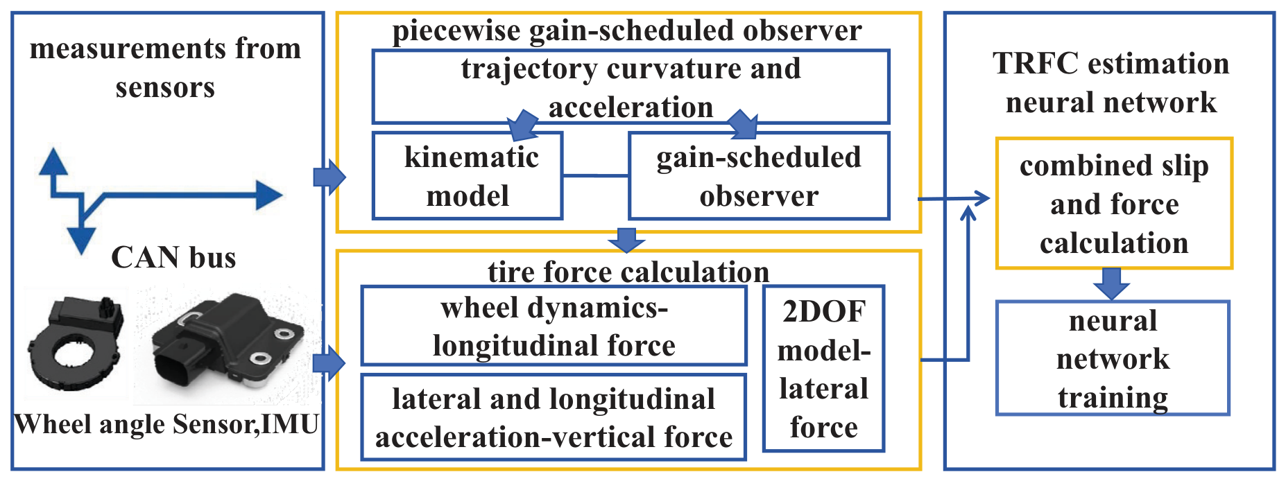
This paper investigates TRFC estimation based on low-cost IMU sensors. As shown in Figure 1, the overall framework includes four core modules that rely on measurements from wheel rotation angle sensors and IMU devices. A three-dimensional vehicle kinematic model containing roll rate, pitch rate, and yaw rate parameters is established. Based on the time-varying characteristics of these angular rates, a piecewise lateral velocity observer is designed with gain scheduling adapted to diverse vehicle motion states. The tire longitudinal, lateral, and vertical forces are calculated by combining the vehicle lateral dynamic model, vertical dynamic model, and wheel rotation dynamic model. After the lateral velocity and tire forces are obtained, the combined slip states and force information of each tire can be computed and delivered to the neural network for TRFC estimation.

In this work, a 2-DOF vehicle dynamic model is employed for the calculation of lateral forces acting on the front and rear axles. Four independent wheel dynamic models are utilized to acquire tire longitudinal forces. Furthermore, a high-fidelity full-vehicle dynamic model embedded in CarSim is adopted to validate the performance of the proposed observer.

2.2. Kinematic Model

Tire dynamics incorporate the coupling effects of TRFC, tire slip characteristics (including longitudinal slip ratio and sideslip angle), and tire forces [48]. Therefore, accurate acquisition of tire slip states and tire forces is a prerequisite for reliable TRFC estimation via tire dynamic responses. Tire slip and tire force variations are highly correlated with tire velocity, which is determined by vehicle lateral velocity. In this study, a three-dimensional vehicle kinematic model containing longitudinal, lateral, and vertical velocity dynamics is adopted for lateral velocity observer design. $a_x$, $a_y$, and $a_z$ denote the longitudinal, lateral, and vertical accelerations, respectively; p, q, and r represent the roll rate, pitch rate, and yaw rate, respectively; $\theta$ and $\varphi$ are the vehicle pitch angle and roll angle, respectively; and $v_x$, $v_y$, and $v_z$ denote the longitudinal, lateral, and vertical velocities, respectively. All acceleration and angular rate signals can be acquired from low-cost IMU sensors. By defining the input vector as $u={[a_x,a_y,a_z]}^{\top }$ and the state vector as $x={[v_x,v_y,v_z]}^{\top }$, the following state-space equations can be obtained:

$$\dot{x}=Ax+Bu+\omega$$

(1)

where

$$A=\left[\begin{array}{ccc}0& r& -q\\ -r& 0& p\\ q& -p& 0\end{array}\right]B=\left[\begin{array}{ccc}1& 0& 0\\ 0& 1& 0\\ 0& 0& 1\end{array}\right]\omega =\left[\begin{array}{c}g\sin \theta \\ -g\cos \theta \sin \varphi \\ -g\cos \theta \cos \varphi \end{array}\right],$$

and g denotes the gravitational acceleration. The above formulation represents a linear time-varying model. In practical driving scenarios, vehicle roll, pitch, and angular rates continuously vary with complex and changeable operating conditions. To facilitate observer design, a polytopic linear-parameter-varying (LPV) model is established. All time-varying angular rate parameters are constrained within bounded intervals, expressed as:

$$\begin{array}{c}\hfill p\in [\underline{p},\overline{p}]q\in [\underline{q},\overline{q}]r\in [\underline{r},\overline{r}].\end{array}$$

(2)

For 4WID vehicles, the longitudinal velocity at the vehicle center of gravity (CG) can be acquired using the method proposed in [49]. Therefore, the longitudinal velocity can be reasonably regarded as the measurable system output. By defining $ϵ={[p,q,r]}^{\top }$ as the time-varying parameter vector, the system LPV model is formulated as [50,51]:

$$\begin{array}{cc}\hfill \dot{x}& =A\left(ϵ\right)x+Bu+\omega ={\displaystyle \sum _{i=1}^{2^3}}{\beta }_i{A}_i+Bu+\omega \hfill \\ \hfill y& =Cx,C=[1,0,0],\hfill \end{array}$$

(3)

where the time-varying weighting coefficients ${\beta }_i$ are expressed as:

$$\begin{array}{c}\hfill {\beta }_1={\displaystyle \frac{(p-\underline{p})(q-\underline{q})(r-\underline{r})}{(\overline{p}-\underline{p})(\overline{q}-\underline{q})(\overline{r}-\underline{r})}}{\beta }_2={\displaystyle \frac{(p-\underline{p})(\overline{q}-q)(r-\underline{r})}{(\overline{p}-\underline{p})(\overline{q}-\underline{q})(\overline{r}-\underline{r})}}\\ \hfill {\beta }_3={\displaystyle \frac{(\overline{p}-p)(q-\underline{q})(r-\underline{r})}{(\overline{p}-\underline{p})(\overline{q}-\underline{q})(\overline{r}-\underline{r})}}{\beta }_4={\displaystyle \frac{(p-\underline{p})(q-\underline{q})(\overline{r}-r)}{(\overline{p}-\underline{p})(\overline{q}-\underline{q})(\overline{r}-\underline{r})}}\\ \hfill {\beta }_5={\displaystyle \frac{(p-\underline{p})(\overline{q}-q)(\overline{r}-r)}{(\overline{p}-\underline{p})(\overline{q}-\underline{q})(\overline{r}-\underline{r})}}{\beta }_6={\displaystyle \frac{(\overline{p}-p)(q-\underline{q})(\overline{r}-r)}{(\overline{p}-\underline{p})(\overline{q}-\underline{q})(\overline{r}-\underline{r})}}\\ \hfill {\beta }_7={\displaystyle \frac{(\overline{p}-p)(\overline{q}-q)(r-\underline{r})}{(\overline{p}-\underline{p})(\overline{q}-\underline{q})(\overline{r}-\underline{r})}}{\beta }_8={\displaystyle \frac{(\overline{p}-p)(\overline{q}-q)(\overline{r}-r)}{(\overline{p}-\underline{p})(\overline{q}-\underline{q})(\overline{r}-\underline{r})}}\end{array}$$

and the vertex system matrices $A_i$ are given by:

$$\begin{gathered} A_1=\left[\begin{array}{ccc}0& \overline{r}& -\overline{q}\\ -\overline{r}& 0& \overline{p}\\ \overline{q}& -\overline{p}& 0\end{array}\right]A_2=\left[\begin{array}{ccc}0& \overline{r}& -\underline{q}\\ -\overline{r}& 0& \overline{p}\\ \underline{q}& -\overline{p}& 0\end{array}\right] \\ {A}_3=\left[\begin{array}{ccc}0& \overline{r}& -\overline{q}\\ -\overline{r}& 0& \underline{p}\\ \overline{q}& -\underline{p}& 0\end{array}\right]A_4=\left[\begin{array}{ccc}0& \underline{r}& -\overline{q}\\ -\underline{r}& 0& \overline{p}\\ \overline{q}& -\overline{p}& 0\end{array}\right] \\ {A}_5=\left[\begin{array}{ccc}0& \underline{r}& -\underline{q}\\ -\underline{r}& 0& \overline{p}\\ \underline{q}& -\overline{p}& 0\end{array}\right]A_6=\left[\begin{array}{ccc}0& \underline{r}& -\overline{q}\\ -\underline{r}& 0& \underline{p}\\ \overline{q}& -\underline{p}& 0\end{array}\right] \\ {A}_7=\left[\begin{array}{ccc}0& \overline{r}& -\underline{q}\\ -\overline{r}& 0& \underline{p}\\ \underline{q}& -\underline{p}& 0\end{array}\right]A_8=\left[\begin{array}{ccc}0& \underline{r}& -\underline{q}\\ -\underline{r}& 0& \underline{p}\\ \underline{q}& -\underline{p}& 0\end{array}\right]. \end{gathered}$$

In Equation (3), $A_i$ denotes the system matrix corresponding to each parameter vertex.

2.3. Observability Condition Based on Vehicle 3-DOF Dynamic Model

After establishing the vehicle LPV kinematic model (3), a dedicated lateral velocity observer is designed based on the proposed model. Sufficient system observability is a fundamental prerequisite for reliable state estimation, which is analyzed in detail in this subsection. According to the observability criterion for linear time-invariant systems, the system (1) with longitudinal velocity as the measurable output is fully observable if and only if the rank of the observability matrix equals the system state dimension:

$$\mathrm{rank}{\left[\begin{array}{ccc}C\hfill & CA\hfill & C{A}^2\hfill \end{array}\right]}^{\top }=3.$$

(4)

The above rank condition can be further simplified into a concise mathematical constraint:

$$p(q^2+r^2)\ne 0.$$

(5)

Based on the established LPV kinematic model, system observability serves as the essential prerequisite for reliable lateral velocity estimation. According to the rank criterion for linear systems, the studied system is fully observable if and only if $p(q^2+r^2)\ne 0$. This mathematical condition reveals a prominent problem in practical vehicle applications.

In routine driving scenarios such as straight-line cruising, constant-speed travel on flat roads, and steady acceleration or deceleration, the vehicle maintains a stable posture without obvious steering, pitching, or rolling movements. Under these operating conditions, the roll rate p, pitch rate q, and yaw rate r measured by IMU sensors gradually approach zero. As $p\to 0$, $q\to 0$, and $r\to 0$, the time-varying system matrix $A\left(ϵ\right)$ becomes nearly singular and suffers from severe ill-conditioning. Such an ill-conditioned system matrix reduces the rank richness of the observability matrix, weakens dynamic excitation for unmeasured states, and consequently leads to degraded or even complete loss of system observability.

Conventional fixed-gain observers adopt uniform parameters for all driving conditions. They achieve satisfactory estimation performance under high-dynamic scenarios where p, q, and r maintain large magnitudes and the system remains fully observable. However, under low-excitation steady-state conditions with near-zero angular rates, insufficient state excitation causes slow error convergence and cumulative estimation deviations. Such performance degradation can be further amplified when the vehicle switches to transient maneuvers, including sharp turning and slope driving.

Since system observability is highly dependent on the magnitude and sign of p, q, and r, the overall driving envelope exhibits distinct piecewise observability characteristics under different vehicle maneuvers. To address the time-varying observability degradation problem, this paper partitions the full vehicle operating range into multiple subdomains according to the variation rules of roll rate, pitch rate, and yaw rate. A piecewise gain-scheduled observer is correspondingly designed to adapt observer gains to time-varying observability levels, ensuring stable and accurate state estimation under both steady-state low-excitation and dynamic high-excitation driving conditions. This research develops a generic piecewise observer design methodology that considers the effects of path curvature, vehicle acceleration, and road slope on system observability conditions.

2.4. Gain-Scheduled Piecewise Velocity Observer Design

An observer design method is formulated for system (3) under satisfied observability conditions. For 4WID vehicles, the operating ranges of roll, pitch, and yaw rates can be divided into N independent intervals. For the k-th interval, the parameter upper and lower bounds are defined as ${\overline{p}}^k$, ${\underline{p}}^k$, ${\overline{q}}^k$, ${\underline{q}}^k$, ${\overline{r}}^k$, and ${\underline{r}}^k$, where $k=1,2,\dots ,N$. The corresponding piecewise observer for the k-th interval is constructed as:

$$\begin{array}{cc}\hfill \dot{\widehat{x}}& ={\displaystyle \sum _{i=1}^{2^3}}{\beta }_i{A}_i^k\widehat{x}+Bu+L^k(y-\widehat{y})\hfill \\ \hfill \widehat{y}& =C\widehat{x},C=[1,0,0],\hfill \end{array}$$

(6)

where $\widehat{x}$ denotes the estimated system state, $A_i^k$ represents the i-th vertex system matrix corresponding to the k-th parameter interval, $L^k$ is the scheduled observer gain for the k-th interval, and $\widehat{y}$ indicates the estimated system output.

Define the observation error as $e=x-\widehat{x}$. By differentiating the error dynamics and substituting the system model (3) and observer formulation (6), the dynamic equation of the observation error is derived as:

$$\dot{e}={\displaystyle \sum _{i=1}^{2^3}}{\beta }_i(A_i^k-L_i^{k}C)e+\omega .$$

(7)

The core objective of the designed gain-scheduled observer is to obtain the observer gains $L_i^k$ such that the observation error system is asymptotically stable with a satisfactory convergence speed and guaranteed $H_{\infty }$ disturbance attenuation performance. The required stability and performance constraints are formulated as follows.

The error system (7) is asymptotically stable with all poles confined within the predefined domain $\mathbb{D}=\{x+jy|-b^k<x<-a^k\}$ and satisfies the $H_{\infty }$ performance index:

$$\begin{array}{c}\hfill \underset{{\left|\right|\omega \left|\right|}_2\ne 0}{\sup }{\displaystyle \frac{{\left|\right|e\left|\right|}_2}{{\left|\right|\omega \left|\right|}_2}}\le \gamma \end{array}$$

if a symmetric positive-definite matrix $P>0$ and nonnegative scalar $\gamma$, as well as rectangular matrices $M_i^k$ exist, such that the following linear matrix inequalities (LMIs) hold [52]:

$$\begin{array}{c}\hfill \left[\begin{array}{cc}{A_i^k}^{\top }P+P{A}_i^k-C^{\top }{M_i^k}^{\top }-M_i^{k}C+I& -M_i^k\\ \ast & -{\gamma }^2\end{array}\right]<0\end{array}$$

(8)

$$\begin{array}{c}\hfill {A_i^k}^{\top }P+P{A}_i^k-C^{\top }{M_i^k}^{\top }-M_i^{k}C+2b^{k}P<0\end{array}$$

(9)

$$\begin{array}{c}\hfill {A_i^k}^{\top }P+P{A}_i^k-C^{\top }{M_i^k}^{\top }-M_i^{k}C+2a^{k}P>0,\end{array}$$

(10)

where the observer gain matrix $L_i^k$ can be calculated by:

$$\begin{array}{c}\hfill L_i^k=P^{-1}{M}_i^k.\end{array}$$

(11)

In Equation (8), I denotes the identity matrix. The LMI constraint (8) guarantees the $H_{\infty }$ disturbance attenuation capability of the proposed observer against external disturbances $\omega$. The pole placement constraints (9) and (10) confine all poles of the error dynamic system within the prescribed domain $\mathbb{D}$, enabling the observation error to converge to zero at a controllable and rapid rate. Since the above constraints are valid for all vertex matrices $A_i^k$ ($i=1,\dots ,2^3$), the uniform $H_{\infty }$ performance and stable convergence performance can be ensured for all parameter variations within the predefined intervals across all N subdomains.

The unknown matrices P, $M_i^k$ and the disturbance attenuation coefficient $\gamma$ are determined by transforming the corresponding inequality constraints into a convex optimization problem which can be solved via the LMI toolbox in MATLAB. The optimization problem is formulated as:

$$\begin{array}{cc}\hfill & {\min }_{P>0,M_i^k,\gamma >0}\gamma \hfill \\ \hfill & \mathrm{s}.\mathrm{t}.\hfill \\ \hfill & \left[\begin{array}{cc}{A_i^k}^{\top }P+P{A}_i^k-C^{\top }{M_i^k}^{\top }-M_i^{k}C+I& -M_i^k\\ \ast & -{\gamma }^2\end{array}\right]<0,\hfill \\ \hfill & {A_i^k}^{\top }P+P{A}_i^k-C^{\top }{M_i^k}^{\top }-M_i^{k}C+2b^{k}P<0,\hfill \\ \hfill & -\left({A_i^k}^{\top }P+P{A}_i^k-C^{\top }{M_i^k}^{\top }-M_i^{k}C+2a^{k}P\right)<0,\hfill \\ \hfill & \forall i,k.\hfill \end{array}$$

(12)

After the optimal matrices P and $M_i^k$ are obtained, the local vertex observer gains $L_i^k$ are calculated via $L_i^k=P^{-1}{M}_i^k$. The final time-varying observer gain for each parameter interval is synthesized through convex combination of all vertex gains, expressed as:

$$L^k={\displaystyle \sum _{i=1}^8}{\beta }_i{L}_i^k.$$

(13)

The piecewise design principle is developed according to the sign and magnitude variation characteristics of roll, pitch, and yaw rates. The system observability condition holds for arbitrary positive or negative signs of the three angular rates. Variations in angular rate signs and magnitudes correspond to different parameter subdomains, which require matched observer gain sets to maintain stable estimation performance. The complete implementation procedure of the proposed piecewise gain-scheduled observer is summarized in Algorithm 1.

Algorithm 1 A piecewise gain-scheduled lateral velocity observer design algorithm

Require: $p,q,r,{\overline{p}}^k,{\underline{p}}^k,{\overline{q}}^k,{\underline{q}}^k,{\overline{r}}^k,{\underline{r}}^k,k=1,2,\dots ,N$ Ensure: Interval-adaptive observer gain $L^k$  1: while $k\le N$ do  2:     Substitute interval bounds ${\overline{p}}^k,{\underline{p}}^k,{\overline{q}}^k,{\underline{q}}^k,{\overline{r}}^k,{\underline{r}}^k$ into the LPV model (3)  3:     Solve the LMI constraints (8)–(10)  4:     Calculate vertex observer gains $L_i^k$ via (11)  5:     Compute time-varying weighting coefficients ${\beta }_i$ using real-time $p,q,r$ measurements  6:     Synthesize the interval observer gain $L^k$ via (13)  7:     $k\leftarrow k+1$  8: end while  9: return $L^k$

With the implementation of Algorithm 1, the signs and magnitudes of IMU-measured p, q, and r are matched with predefined parameter intervals to determine the optimal operating subdomain k. Corresponding vertex gains $L_i^k$ are solved based on the interval parameter bounds, and the real-time observer gain is synthesized using convex weighting coefficients. With the proposed observer, vehicle lateral velocity can be accurately estimated, and the estimation error can converge rapidly and steadily. The reliable lateral velocity estimation further supports the subsequent calculation of tire velocity states, tire slip parameters, and tire dynamic forces, which provides accurate state inputs for the TRFC estimation module in the following section.

3. Combined Slip Calculations and Estimation Neural Network

3.1. Tire Slip and Force

Wheel slip and tire force are essential for TRFC estimation. The wheel slip and force definitions presented in [48] are adopted in this study. Let $r_e$ denote the effective rolling radius of a wheel. The longitudinal slip ratio $\kappa$ of the wheel is defined as:

$$\kappa ={\displaystyle \frac{{\omega }_w{r}_e-v_x^{\mathrm{tire}}}{max({\omega }_w{r}_e,v_x^{\mathrm{tire}})}},$$

(14)

where ${\omega }_w$ is the wheel rotational speed, and $v_x^{\mathrm{tire}}$ denotes the longitudinal velocity at the wheel center.

The tire lateral slip angle $\alpha$ is defined as the angle between the tire heading direction and the velocity vector of the wheel:

$$tan\alpha ={\delta }^{\mathrm{tire}}-{\theta }_v^{\mathrm{tire}},$$

(15)

where ${\delta }^{\mathrm{tire}}$ is the tire steering angle, and ${\theta }_v^{\mathrm{tire}}$ represents the angle between the wheel velocity vector and the vehicle longitudinal axis.

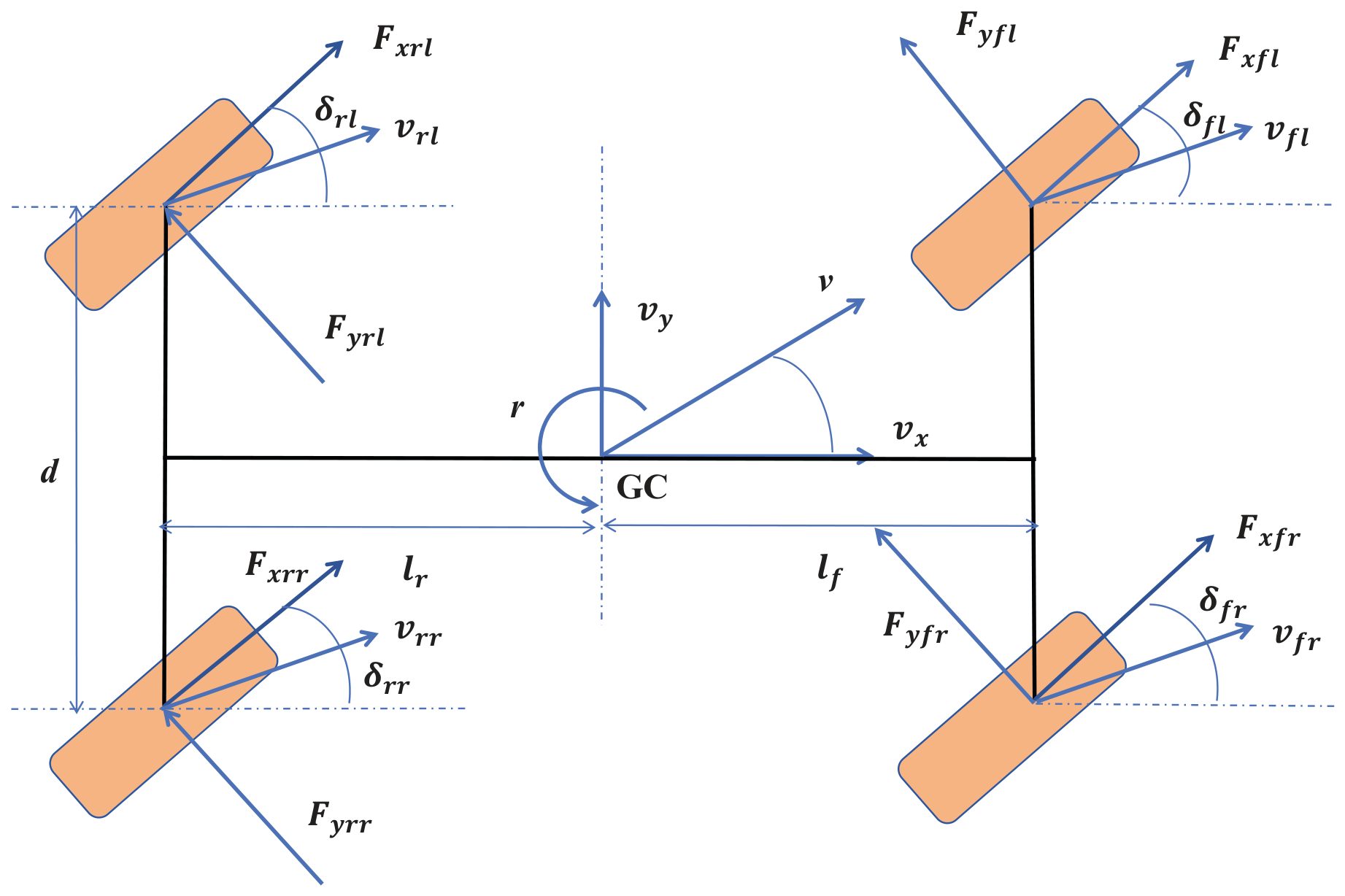
Using the vehicle lateral velocity and yaw rate at the center of gravity (CG) shown in Figure 2, the velocity at each wheel center is calculated as:

$$\begin{array}{cc}\hfill v_{\mathrm{fl}}& =(v_x-rd/2)cos\left({\delta }_{\mathrm{fl}}\right)+(v_y+r{l}_f)sin\left({\delta }_{\mathrm{fl}}\right)\hfill \\ \hfill v_{\mathrm{fr}}& =(v_x+rd/2)cos\left({\delta }_{\mathrm{fr}}\right)+(v_y+r{l}_f)sin\left({\delta }_{\mathrm{fr}}\right)\hfill \\ \hfill v_{\mathrm{rl}}& =(v_x-rd/2)cos\left({\delta }_{\mathrm{rl}}\right)+(v_y-r{l}_r)sin\left({\delta }_{\mathrm{rl}}\right)\hfill \\ \hfill v_{\mathrm{rr}}& =(v_x+rd/2)cos\left({\delta }_{\mathrm{rr}}\right)+(v_y-r{l}_r)sin\left({\delta }_{\mathrm{rr}}\right),\hfill \end{array}$$

(16)

where $v_{\mathrm{fl}}$, $v_{\mathrm{fr}}$, $v_{\mathrm{rl}}$ and $v_{\mathrm{rr}}$ are the velocities of the front-left, front-right, rear-left and rear-right tires, respectively; $l_f$ and $l_r$ are the distances from the front and rear axles to the CG; ${\delta }_i$ stands for the steering angle of tire i with $i\in \{\mathrm{fl},\mathrm{fr},\mathrm{rl},\mathrm{rr}\}$; $v_x$ and $v_y$ are the longitudinal and lateral velocities at the CG, and d denotes the wheel track.

After acquiring wheel velocities, the longitudinal slip ratio and sideslip angle of each tire can be computed. According to Equation (14), the slip ratio of each wheel ${\kappa }_i$ and the sideslip angle of each wheel ${\alpha }_i$ can be obtained [53].

Small angle approximations yield the following tire slip angle formulations:

$$\begin{array}{cc}\hfill {\alpha }_{\mathrm{fl}}& ={\delta }_{\mathrm{fl}}-{\displaystyle \frac{v_y+r{l}_f}{v_x-rd/2}},{\alpha }_{\mathrm{fr}}={\delta }_{\mathrm{fr}}-{\displaystyle \frac{v_y+r{l}_f}{v_x+rd/2}}\hfill \\ \hfill {\alpha }_{\mathrm{rl}}& ={\delta }_{\mathrm{rl}}-{\displaystyle \frac{v_y-r{l}_r}{v_x-rd/2}},{\alpha }_{\mathrm{rr}}={\delta }_{\mathrm{rr}}-{\displaystyle \frac{v_y-r{l}_r}{v_x+rd/2}}.\hfill \end{array}$$

(17)

The longitudinal slip ratio and sideslip angle for each tire are now obtained. Subsequent discussions focus on tire force calculation, where a 2-DOF vehicle lateral dynamic model is adopted for this purpose. The estimated lateral forces of the front and rear axles are written as [2]:

$$\begin{array}{cc}\hfill F_{y1}& ={\displaystyle \frac{m{l}_r({\dot{v}}_y+v_{x}r)+I_z\dot{r}}{l_f+l_r}}\hfill \\ \hfill F_{y2}& ={\displaystyle \frac{m{l}_f({\dot{v}}_y+v_{x}r)-I_z\dot{r}}{l_f+l_r}},\hfill \end{array}$$

(18)

where $F_{y1}$ and $F_{y2}$ are the total lateral forces of the front and rear axles, respectively, and $I_z$ is the vehicle yaw moment of inertia about the CG.

The 2-DOF lateral model is selected considering the practical requirement of real-time on-board estimation. This model accurately describes the overall lateral and yaw motion characteristics of the vehicle and calculates the total lateral force at the axle level rather than individual tire force. Since axle-level resultant forces are dominated by global vehicle motion and are insensitive to local combined slip effects of single tires, the 2-DOF model maintains satisfactory accuracy for axle lateral force computation under combined slip conditions. Compared with high-fidelity full-vehicle models, it achieves a good balance between model fidelity and computational efficiency, which matches the low-cost and real-time application orientation of this work.

The vertical load of each wheel is calculated by considering longitudinal and lateral load transfer [2]:

$$\begin{array}{cc}\hfill F_{z\mathrm{fl}}& ={\displaystyle \frac{mg{l}_r}{2l}}-{\displaystyle \frac{m{a}_{x}h}{2l}}-{\displaystyle \frac{m{a}_{y}h{l}_f}{dl}}\hfill \\ \hfill F_{z\mathrm{fr}}& ={\displaystyle \frac{mg{l}_r}{2l}}-{\displaystyle \frac{m{a}_{x}h}{2l}}+{\displaystyle \frac{m{a}_{y}h{l}_f}{dl}}\hfill \\ \hfill F_{z\mathrm{rl}}& ={\displaystyle \frac{mg{l}_f}{2l}}+{\displaystyle \frac{m{a}_{x}h}{2l}}-{\displaystyle \frac{m{a}_{y}h{l}_r}{dl}}\hfill \\ \hfill F_{z\mathrm{rr}}& ={\displaystyle \frac{mg{l}_f}{2l}}+{\displaystyle \frac{m{a}_{x}h}{2l}}+{\displaystyle \frac{m{a}_{y}h{l}_r}{dl}},\hfill \end{array}$$

(19)

where subscript z denotes the vertical direction of tire forces.

It is noted that the adopted model does not explicitly incorporate road roughness, suspension dynamics, and structural flexibility. These factors introduce bounded time-varying disturbances to tire vertical loads and tire forces. Nevertheless, the designed piecewise gain-scheduled observer with $H_{\infty }$ robustness can effectively suppress such unmodeled dynamics and external disturbances, ensuring stable estimation performance under general driving conditions on paved roads. For extreme operating conditions with prominent suspension vibration or structural deformation, high-order full-vehicle models will be adopted in future research to further improve model accuracy.

Based on the axle lateral forces in Equation (18), the lateral force of each single tire is derived by proportional distribution according to tire vertical loads [1]:

$$\begin{array}{cc}\hfill F_{y\mathrm{fl}}& ={\displaystyle \frac{F_{z\mathrm{fl}}}{F_{z\mathrm{fl}}+F_{z\mathrm{fr}}}}{F}_{y1},F_{y\mathrm{fr}}={\displaystyle \frac{F_{z\mathrm{fr}}}{F_{z\mathrm{fl}}+F_{z\mathrm{fr}}}}{F}_{y1}\hfill \\ \hfill F_{y\mathrm{rl}}& ={\displaystyle \frac{F_{z\mathrm{rl}}}{F_{z\mathrm{rl}}+F_{z\mathrm{rr}}}}{F}_{y2},F_{y\mathrm{rr}}={\displaystyle \frac{F_{z\mathrm{rr}}}{F_{z\mathrm{rl}}+F_{z\mathrm{rr}}}}{F}_{y2},\hfill \end{array}$$

(20)

where subscript y represents the lateral direction of tire forces.

This load-proportional distribution is a widely used engineering simplification, which is valid for normal driving conditions within moderate dynamic ranges. Under combined slip and extreme driving scenarios, tire nonlinearity, camber angle, structural flexibility and tire force saturation will break this linear distribution rule. The present work focuses on combined slip conditions in regular driving ranges, where this simplification yields acceptable accuracy. For severe extreme maneuvers, improved distribution models considering tire nonlinear characteristics will be adopted in follow-up studies.

The rotational dynamics of the four wheels are established as:

$$I_w{\dot{\omega }}_i=T_i-T_{bi}-F_{xi}{R}_w,$$

(21)

where $I_w$ is the wheel moment of inertia, $T_i$ is the driving torque of the in-wheel motor for wheel i, $T_{bi}$ is the braking torque, subscript x denotes the longitudinal direction, and $R_w$ is the wheel rolling radius.

Rearranging Equation (21), the longitudinal force of each tire is solved as:

$$F_{xi}={\displaystyle \frac{T_i-T_{bi}-I_w{\dot{\omega }}_i}{R_w}}.$$

(22)

At this stage, tire slip states and tire forces are fully acquired. Under combined slip conditions, longitudinal and lateral tire forces exhibit strong coupling effects. Therefore, the original slip definitions for pure slip scenarios need to be further processed, which is discussed in the following subsection.

3.2. TRFC Prediction Network

The slip definitions in Equations (14) and (15) are established for pure slip cases and cannot directly describe combined slip characteristics. To ensure the accuracy of the TRFC estimation method, the slip values derived from (14) and (15) are processed accordingly. Referring to the standard tire modeling method in [48], theoretical normalized slip quantities are introduced:

$$\begin{array}{c}\hfill {\delta }_x={\displaystyle \frac{\kappa }{1+\left|\kappa \right|}}{\delta }_y={\displaystyle \frac{tan\alpha }{1+\left|\kappa \right|}},\end{array}$$

(23)

where $\kappa$ is the longitudinal slip ratio, $\alpha$ is the tire sideslip angle, ${\delta }_x$ and ${\delta }_y$ denote the normalized longitudinal and lateral slips, respectively.

The tire forces calculated from Equations (19), (20) and (22) are also fused to obtain the resultant tire force $F_w$:

$$F_w=\sqrt{F_x^2+F_y^2}.$$

(24)

Intelligent algorithms have been widely applied to improve vehicle safety and operation efficiency [54]. Different from traditional empirical tire models, data-driven machine learning is adopted here for TRFC estimation. As a typical machine learning structure, artificial neural networks (ANNs) originate from the simulation of biological neural connections [55,56]. Multilayer perceptron (MLP), as a classic ANN, has been proven capable of approximating arbitrary nonlinear functions with high precision [57,58]. A multilayer perceptron is employed to train the TRFC estimation network.

The development of the TRFC estimation network includes data collection, network training and performance testing. In this work, the dataset is initially generated via co-simulation in CarSim under various combined slip conditions. The collected variables contain tire longitudinal force, lateral force, vertical force, longitudinal slip ratio, sideslip angle and reference tire–road friction coefficient. All raw variables are processed via Equations (23) and (24) to construct normalized combined slip and resultant force features. The processed combined slip, resultant tire force and vertical tire load are taken as network inputs, while the TRFC is set as the network output.

Simulation data from CarSim are adopted in the algorithm verification phase due to its advantages of full-condition controllability, low cost and zero test risk. CarSim embedded with the Pacejka tire model can faithfully reproduce tire mechanical characteristics under diverse slip and friction conditions. However, it is acknowledged that datasets generated purely by simulation may cause the network to overfit simulator inherent features, leading to limited generalization capability in real-vehicle applications. To mitigate this problem, two optimization strategies can be adopted in the future. First, the working condition coverage is expanded on the basis of the original settings; Gaussian noise is superimposed on simulation data to simulate real sensor noise and unmodeled errors. Second, real-vehicle test data collected from actual road environments will be combined with simulation data to build a mixed dataset for network retraining in practical applications, so as to narrow the gap between simulation and real scenarios.

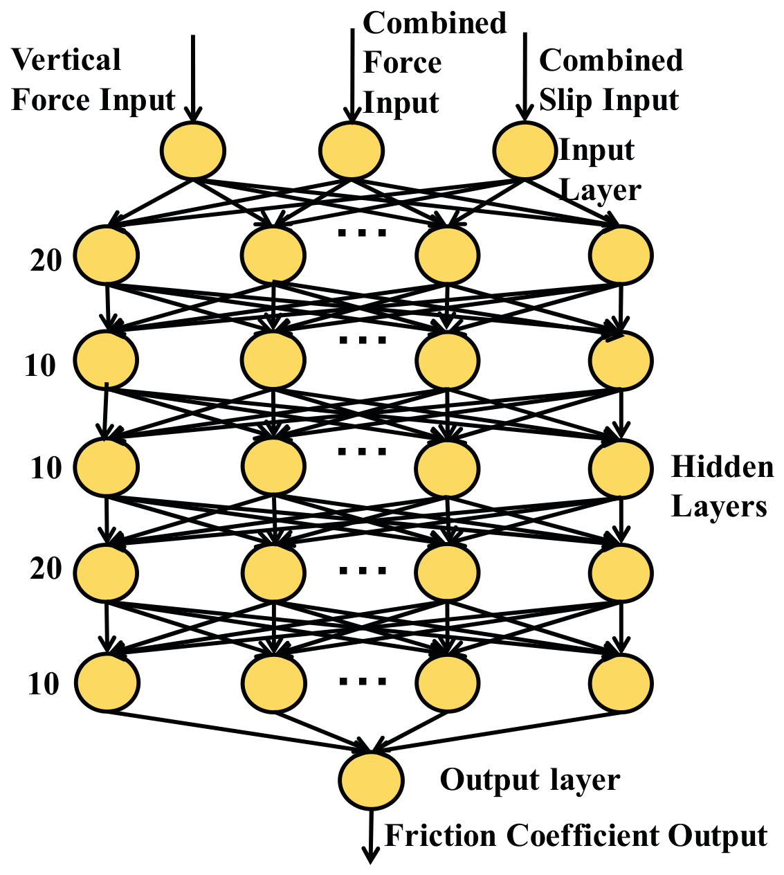
The data variation ranges and intervals are listed in

Table 1. Ranges of tire test data variation.

Input	Variation Range	Increment
Slip Ratio	$[0.55,0.85]$	$0.05$
Sideslip Angle (deg)	$[1,10]$	1
Friction Coefficient	$[0.1,0.9]$	$0.1$
Vertical Force (N)	$[2000,4000]$	500

. The input values vary incrementally over their respective preset ranges, as listed in Table 1. It is worth mentioning that negative slip ratios commonly appear during braking, and large slip values may occur in critical driving scenarios. The introduced normalized slip definitions in Equation (23) can effectively handle such operating cases. A total of 50,000 samples are generated from CarSim. According to standard dataset partitioning rules, 80% of samples are randomly selected as the training set, and the remaining 20% are used as the test set. The number of neurons in each hidden layer and the overall network structure is determined through trial-and-error tests, and the final MLP structure is illustrated in Figure 3.

Remark 1.

The proposed method separates offline design and online execution: the observer gain solution and network training are completed offline, while the online algorithm only involves simple matrix operations and network forward propagation. The fixed sampling time is set as 0.001 s, which fully meets the real-time requirement of vehicle embedded systems.

4. Simulation Studies

This section presents the numerical validation of the dynamic model in (1), the designed observer, and the tire–road friction coefficient (TRFC) estimation method. Comprehensive performance evaluations of the proposed observer are conducted via pure dynamic simulations and CarSim-MATLAB co-simulations.

To fully verify the effectiveness and adaptability of the proposed approach, numerical simulations are implemented under three distinct working conditions. In Case 1, the target trajectory consists of three consecutive circular paths with radii of 152 m, 130 m, and 160 m, yielding continuously varying road curvature. The simulation is performed on a flat road with a constant longitudinal velocity of 30 km/h. Case 2 adopts the identical curvature-varying trajectory as Case 1, while the longitudinal velocity is increased to 60 km/h to explore high-speed driving scenarios. In Case 3, a longitudinal straight path with a 20° road slope is adopted, where the vehicle starts at an initial velocity of 10 km/h and operates in the 4WID mode during uphill driving. Notably, Cases 1 and 2 focus on curvature variation characteristics, whereas Case 3 mainly considers road slope disturbance. The three simulation cases cover typical longitudinal velocities of 10 km/h, 30 km/h, and 60 km/h, enabling a comprehensive assessment of algorithm performance under diverse driving states.

4.1. Model Verification

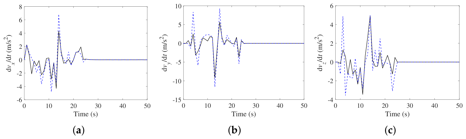
The accuracy of the dynamic model in Equation (1) is verified against the high-fidelity CarSim model under Case 3. Utilizing the parameters p, q, r, $a_x$, $a_y$, $a_z$, $\theta$ and $\varphi$ collected from CarSim for Case 3, the model in Equation (1) is simulated. The calculated ${\dot{v}}_x$, ${\dot{v}}_y$, and ${\dot{v}}_z$ are then compared with the corresponding CarSim outputs. The comparative curves under Case 3 are illustrated in Figure 4. It can be observed that the established dynamic model achieves satisfactory consistency with the high-fidelity CarSim model. Minor deviations still exist between the two sets of results, which are mainly caused by the drastic and frequent variations in angular rates p, q, and r under slope driving conditions. In general, the established model can basically reflect the actual vehicle dynamic characteristics, providing a reliable foundation for subsequent observer design and simulation verification. It should be noted that inevitable mismatches always exist between simplified theoretical models and commercial multi-body dynamic software, and such model errors are also common in numerical simulation studies.

4.2. Lateral Velocity Observer Performance in CarSim

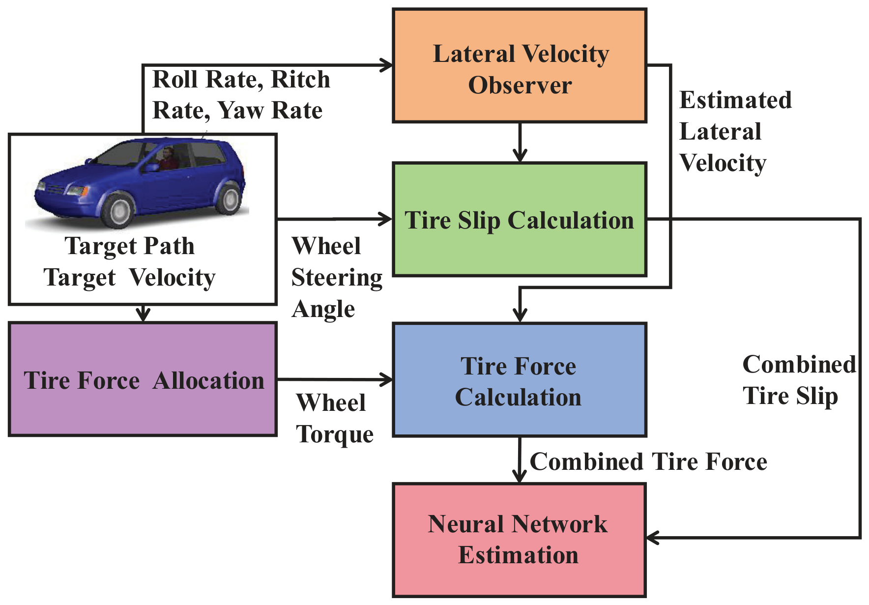
To further demonstrate the performance of the proposed methods, co-simulations between CarSim and MATLAB are carried out. A C-class hatchback vehicle model from CarSim is adopted. A block diagram of the architecture for simulation is shown in Figure 5. It can be seen from Figure 5 that in the co-simulation of MATLAB and CarSim, the lateral speed observer receives roll, pitch, and yaw rate from the CarSim model and transmits the estimated vehicle lateral velocity to the tire slip and force calculation module, which also requires wheel rotation angle signals and torque signals from the CarSim model. In this process, the tire force allocation module for 4WID vehicles is utilized. Tire slip and forces are calculated under combined slip conditions and fed as inputs to the TRFC estimation network.

All simulations adopt $T_s=0.001\mathrm{s}$ to match the working frequency of vehicle electronic systems, and the friction coefficient is limited to $\mu \in [0.1,0.9]$ for physical rationality. Zero-mean Gaussian noise is added to IMU signals, with variance $1\times {10}^{-4}$ for angular velocity and $2\times {10}^{-2}$ for acceleration, conforming to actual sensor noise features. For the KF, $Q=0.05$ and $R=1$ are set to cope with system uncertainty and measurement noise. The particle filter (PF) uses 1000 particles together with multinomial resampling at a ratio of 0.5 to balance accuracy and computation load and avoid particle degeneracy. The sliding mode observer (SM) adopts the standard linear reaching law $\dot{s}={[-1887.39208726.27]}^{\top }s$ with no saturation layer or additional coefficient. The observer gain vector is designed according to the dynamic characteristics of different state variables to realize effective error correction.

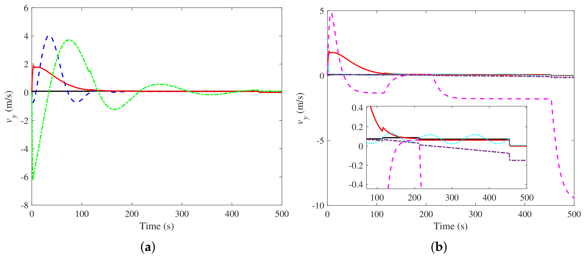
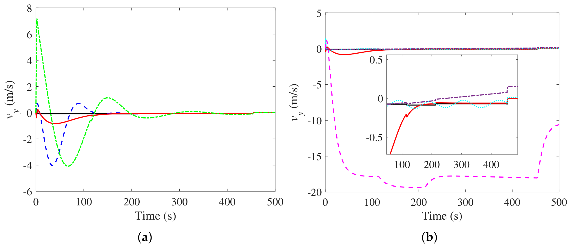
Lateral velocity is the main concerned state variable. The comprehensive comparison results of lateral velocity estimation under various conditions are presented in Figure 6, Figure 7, Figure 8, Figure 9 and Figure 10. Figure 6 compares the estimation performance of the constant gain method, the non-piecewise gain-scheduled method, and the proposed piecewise method under low-speed positive curvature driving conditions. It can be seen that the estimated values of the proposed method can converge well to the real-vehicle state. Compared with the non-piecewise algorithm, the proposed piecewise strategy achieves faster error convergence and higher steady-state accuracy, verifying the effectiveness of the segmented parameter adjustment mechanism. Meanwhile, the proposed method exhibits lower estimation errors than the traditional constant gain observer, demonstrating the superiority of the gain-scheduled adaptive strategy.

The subgraphs in Figure 6 further compare the proposed method with three mainstream observers, including the PF, KF, and SM observer. The KF produces obvious estimation deviations under nonlinear vehicle steering conditions, which is attributed to its inherent dependence on linear system assumptions. In addition, the PF and SM observer suffer from steady-state estimation errors. By contrast, the proposed method achieves the minimum steady-state error and smoother estimation curves under the same working condition.

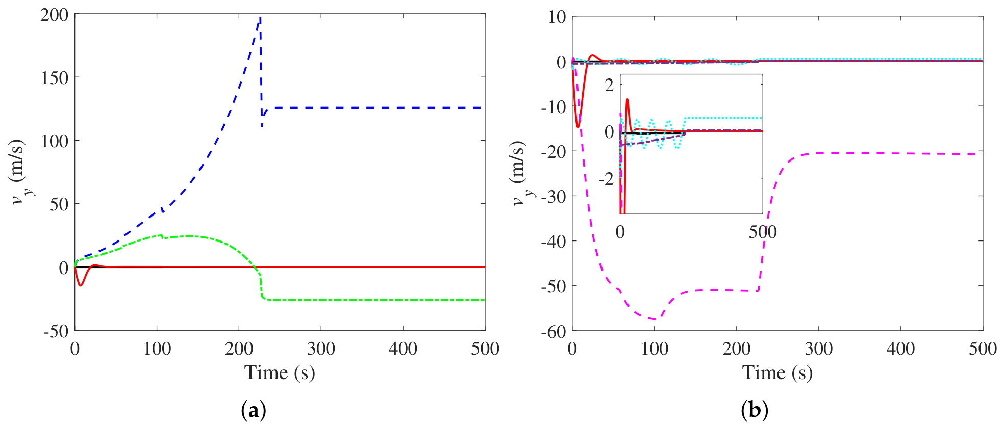
Figure 7 presents the comparison results under high-speed positive curvature driving (Case 2). Obvious performance degradation can be observed for both the constant gain method and the non-piecewise method under high-speed dynamic conditions. Nevertheless, the proposed method maintains stable and accurate estimation performance with minor errors. A slight initial deviation exists in the proposed method, which is caused by the mismatch between the preset initial observer state and the actual vehicle initial state, and such transient error can be gradually eliminated with algorithm iteration.

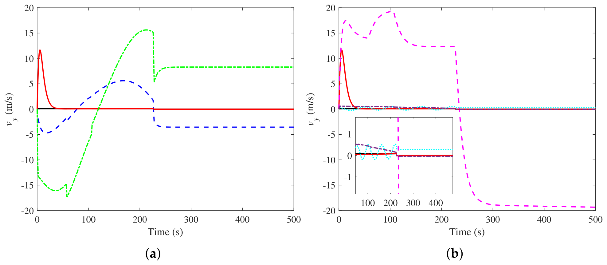
Figure 8 and Figure 9 illustrate the estimation results under negative curvature conditions to validate the algorithm adaptability to different steering directions. Consistent conclusions can be drawn that the proposed piecewise adaptive method outperforms other comparison methods in terms of convergence speed and steady-state accuracy under both low-speed and high-speed reverse steering scenarios.

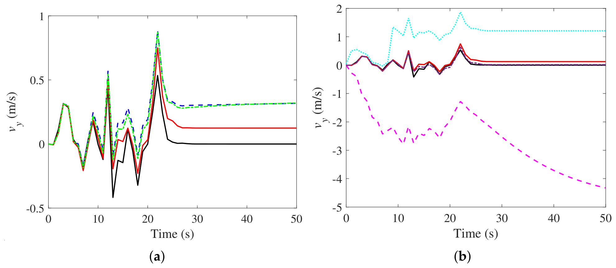
The verification results under slope driving conditions (Case 3) are displayed in Figure 10. The proposed method shows superior performance over the constant gain and non-piecewise methods. However, the performance advantage is relatively limited compared with other advanced observers. This phenomenon is mainly caused by the increased model mismatch between the established theoretical dynamic model and the high-fidelity CarSim model under complex slope driving conditions. It is worth mentioning that all simulation results are obtained under ideal numerical environments without complex road disturbances and sensor faults, so the practical performance in real-vehicle tests may be slightly different from the simulation results.

For a quantitative comparison, we list the Root Mean Square Error (RMSE) and Mean Absolute Error (MAE) to evaluate observer accuracy in

Table 2. Estimation error of different control methods under various working conditions.

Working Condition	Index	Constant Gain	Pro	No-Piecewise	PF	KF	SM
Case 1 with	RMSE	0.0014	0.0144	0.0341	0.0375	19.3073	0.0533
negative curvature	MAE	0.0019	0.0144	0.0441	0.0384	19.3083	0.0535
Case 2 with	RMSE	44.1105	0.1537	24.6661	0.2512	57.3661	0.3504
negative curvature	MAE	44.3511	0.1542	24.7164	0.2829	57.3787	0.3515
Case 1 with	RMSE	0.0014	0.0076	0.4898	0.0285	0.0250	0.0533
positive curvature	MAE	0.0019	0.0076	0.5060	0.0297	0.0251	0.0536
Case 2 with	RMSE	2.0572	0.0335	6.4009	0.3980	19.1390	0.3504
positive curvature	MAE	2.0924	0.0337	6.5268	0.4013	19.1484	0.3514
Case 3	RMSE	0.0002	0.0003	0.0003	0.4032	0.1411	0.0003
	MAE	0.0003	0.0003	0.0003	0.5111	0.2683	0.0003

. From the error results under multiple working conditions, it can be seen that the proposed piecewise controller exhibits outstanding adaptive performance under different scenarios. Under Case 1, the proposed controller maintains low RMSE and MAE values and achieves satisfactory control precision. When facing Case 2, the conventional constant gain controller, non-piecewise controller and KF suffer from sharply increased errors and poor robustness. In contrast, the presented piecewise controller still keeps RMSE and MAE at a low level, which is much better than PF and SM. Under Case 3, the proposed method also maintains high precision consistent with other advanced algorithms. The results demonstrate that the piecewise control strategy can flexibly adjust control parameters according to steering angles and vehicle states, effectively adapt to diverse vehicle steering conditions, and possess strong practicability and robustness for vehicle control systems.

4.3. Friction Coefficient Estimation

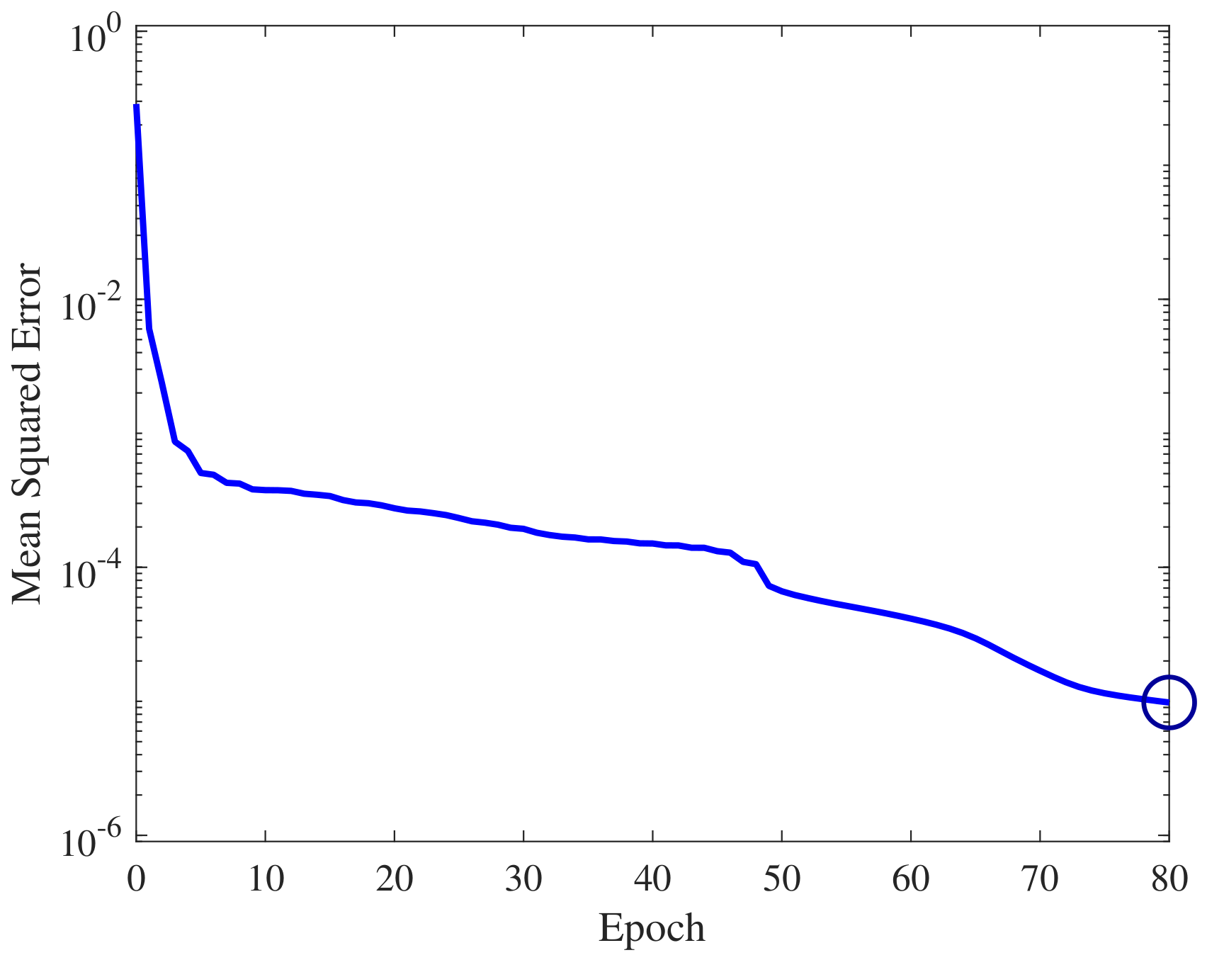
The Artificial Neural Network Toolbox in MATLAB 2018b is employed to train and test the friction coefficient estimation network. The training data set is preprocessed and normalized before training. The performance function is the mean squared error. The training process is implemented offline. During training, the maximum epoch is set to 10,000. The learning rate during training is 0.1 and training stops when the mean squared error is smaller than 0.00001. These parameters are obtained by trial and error tests. The mean squared error across training epochs is plotted in Figure 11. From the plot, it can be observed that the mean squared error gradually decreases and ultimately achieves the training target after approximately 80 epochs. We conduct training under different friction conditions to cover various operating conditions, including split-mu conditions and varying friction levels.

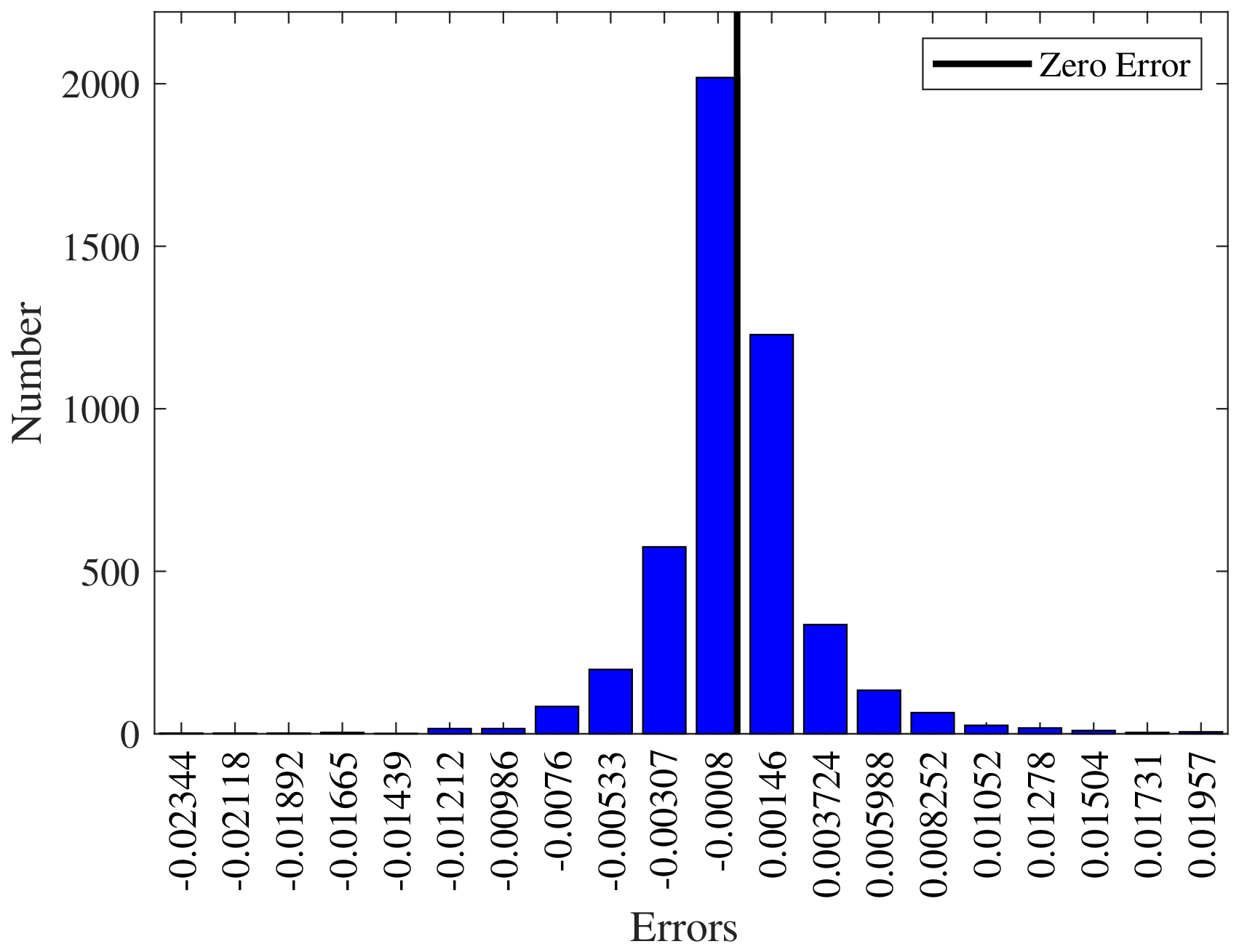
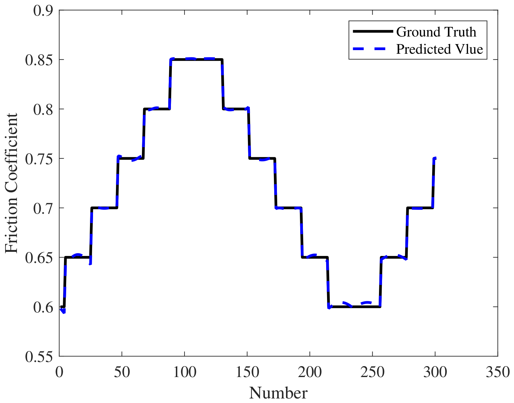
After training, the training error histogram is plotted in Figure 12. The error follows the normal distribution and a large number of errors fall into the range $[-0.003,0.003]$. Figure 13 shows the test result of the designed multilayer perceptron network. This figure indicates that the multilayer perceptron network is well trained and has the ability to estimate the friction coefficient accurately.

To further validate the performance of the friction coefficient estimation network, the estimated lateral velocity, steering angle, longitudinal velocity, and yaw rate of target path 1 are adopted to calculate tire slip values. Then tire forces are calculated by (19)–(21). These values are transmitted to the trained network, and relative estimation errors are shown in

Table 3. Friction coefficient estimation error comparisons.

Methods	Tire Type	Relative Error
proposed	front left tire	0.0154
proposed	front right tire	0.0154
proposed	rear left tire	0.0154
proposed	rear right tire	0.0154
method in [25]	front left tire	−0.0549
method in [25]	front right tire	−0.0549
method in [25]	rear left tire	−0.0549
method in [25]	rear right tire	−0.0549
method in [59]	front left tire	0.3828
method in [59]	front right tire	0.3828
method in [59]	rear left tire	0.3828
method in [59]	rear right tire	0.3828

. It can be discovered that the estimation error of the proposed method is within 2%, which is the smallest compared with methods in [25,59]. This validates the effectiveness of the proposed friction coefficient estimation network. In addition, the estimation error of the proposed method is not zero, which may stem from two aspects: (1) Network regression error, (2) Velocity and force estimation error. In CarSim, the vehicle dynamics are simulated using uniform TRFC for each tire. Furthermore, all four tires of the simulated vehicle are of the same size, specifically 205/55 R16. Consequently, these two factors lead to an identical estimated value of friction coefficient for all tires. It can be deduced from Table 3 that the estimated values are also the same for each tire. This proves that the proposed estimation network is consistent.

4.4. Limitations of This Work

Although the proposed method achieves favorable estimation performance in numerical simulations, it still has several inherent limitations that need to be clarified. First, all validations in this work are exclusively conducted in CarSim/MATLAB simulation environments. Although partial sensor noise is added to simulate imperfect sensing conditions, practical real-vehicle uncertainties, including IMU bias and drift, CAN bus transmission delays, discrete sampling effects, model-parameter mismatch, random road excitation, and time-varying tire characteristics, are not systematically analyzed and quantified. Second, the method relies on simplified modeling assumptions, including the 2-DOF vehicle model and load-proportional tire force distribution under combined slip conditions, which may introduce inevitable modeling errors when applied to complex real driving scenarios. Third, the multilayer perceptron neural network is trained and tested solely on synthetic simulation datasets, lacking real-vehicle measurement data for validation. The generalization ability of the network for diverse practical working conditions and complex external disturbances cannot be fully guaranteed. Overall, the current work only verifies the simulation-level feasibility of the proposed estimation framework, and the practical robustness, real-time performance, and engineering applicability in real-vehicle scenarios remain unvalidated. Hardware-in-the-loop tests and real-vehicle experiments will be carried out in future studies to address the above limitations.

5. Conclusions

This study develops a TRFC estimation method considering combined slip characteristics for 4WID electric vehicles and verifies its feasibility through numerical simulation. Firstly, based on a parameter-varying 3-DOF vehicle model, the observability condition is deduced, and a piecewise gain-scheduled lateral velocity observer is designed. The designed observer satisfies the $H_{\infty }$ performance, guarantees the stability of the estimation error system, and realizes reasonable pole placement to improve the transient response performance of the estimation system. Subsequently, the velocity states, slip values, and dynamic forces of each tire are calculated using the estimated lateral velocity. On this basis, a multilayer perceptron network is constructed to achieve TRFC estimation under combined slip conditions. Simulation results show that the proposed observer yields reduced lateral velocity estimation errors compared with conventional observers without piecewise or gain-scheduled strategies. The proposed method achieves a low relative error of 0.0154 in simulation environments, demonstrating superior numerical estimation performance over benchmark approaches. It is necessary to clarify that this work is limited to simulation-based verification using high-fidelity CarSim models. The adopted vehicle dynamic simplifications and load-proportional tire force distribution strategies are idealized assumptions, which may cause performance deviations under complex practical driving conditions. Additionally, the neural network is trained and tested exclusively on synthetic simulation data, while real-world vehicle uncertainties, including IMU bias and drift, CAN bus delays, sampling errors, parameter mismatch, and time-varying tire characteristics and road disturbances, are not systematically considered in this work. Hardware-in-the-loop and real-vehicle field tests are not included in the current validation, and the practical robustness and engineering applicability of the proposed framework remain unvalidated. Future work will conduct comprehensive experimental tests to further verify the practical performance and engineering applicability of the proposed estimation method for real-vehicle scenarios.

References

1. Liang, Y.; Li, Y.; Khajepour, A.; Zheng, L. Robust path following control of 4WID autonomous vehicle with driving condition adaptive mechanism. Proc. Inst. Mech. Eng. Part D J. Automob. Eng. 2024, 238, 1096–1113. [Google Scholar]
2. Wang, W.; Ma, T.; Yang, C.; Zhang, Y.; Li, Y.; Qie, T. A Path Following Lateral Control Scheme for Four-Wheel Independent Drive Autonomous Vehicle Using Sliding Mode Prediction Control. IEEE Trans. Transp. Electrif. 2022, 8, 3192–3207. [Google Scholar] [CrossRef]
3. Wang, D.; Gu, T.; Zhang, K. Fault Tolerant Control of 4-Wheel Independent Drive Vehicle Subject to Actuator Faults Based on Feasible Region. IEEE Trans. Veh. Technol. 2023, 73, 1652–1666. [Google Scholar] [CrossRef]
4. Tian, M.; Zhang, Q.; Tian, D.; Jin, L.; Li, J.; Xiao, F. Pre-Stability Control for In-Wheel-Motor-Driven Electric Vehicles with Dynamic State Prediction. IEEE Trans. Intell. Veh. 2024, 9, 4541–4554. [Google Scholar] [CrossRef]
5. Cai, Z.; Zhu, X.; Gergondet, P.; Chen, X.; Yu, Z. A Friction-Driven Strategy for Agile Steering Wheel Manipulation by Humanoid Robots. Cyborg Bionic Syst. 2023, 4, 0064. [Google Scholar] [CrossRef] [PubMed]
6. Ko, S.; Ko, J.; Lee, S.; Cheon, J.; Kim, H. A study on the road friction coefficient estimation and motor torque control for an in-wheel electric vehicle. Proc. Inst. Mech. Eng. Part D J. Automob. Eng. 2015, 229, 611–623. [Google Scholar]
7. Wang, J.; Yin, D.; Chen, L.; Du, J. Estimation of road adhesion coefficient for four-wheel independent drive electric vehicle. In Proceedings of the 2020 5th International Conference on Mechanical, Control and Computer Engineering (ICMCCE); IEEE: Piscataway, NJ, USA, 2020; pp. 45–49. [Google Scholar]
8. Hu, J.; Zhang, Y.; Rakheja, S. Adaptive Lane Change Trajectory Planning Scheme for Autonomous Vehicles Under Various Road Frictions and Vehicle Speeds. IEEE Trans. Intell. Veh. 2023, 8, 1252–1265. [Google Scholar]
9. Dogan, D.; Boyraz, P. Smart Traction Control Systems for Electric Vehicles Using Acoustic Road-Type Estimation. IEEE Trans. Intell. Veh. 2019, 4, 486–496. [Google Scholar] [CrossRef]
10. Ma, X.; Dong, Z.; Quan, W.; Dong, Y.; Tan, Y. Real-time assessment of asphalt pavement moduli and traffic loads using monitoring data from Built-in Sensors: Optimal sensor placement and identification algorithm. Mech. Syst. Signal Process. 2023, 187, 109930. [Google Scholar]
11. Wang, H.; Zhang, X.; Jiang, S. A Laboratory and Field Universal Estimation Method for Tire-Pavement Interaction Noise (TPIN) Based on 3D Image Technology. Sustainability 2022, 14, 12066. [Google Scholar] [CrossRef]
12. Wang, Y.; Lv, C.; Yan, Y.; Peng, P.; Wang, F.; Xu, L.; Yin, G. An Integrated Scheme for Coefficient Estimation of Tire-Road Friction with Mass Parameter Mismatch Under Complex Driving Scenarios. IEEE Trans. Ind. Electron. 2022, 69, 13337–13347. [Google Scholar]
13. Rajamani, R. Vehicle Dynamics and Control; Springer: New York, NY, USA, 2012. [Google Scholar]
14. Lecompte, O.; Therrien, W.; Girard, A. Experimental Investigation of a Maneuver Selection Algorithm for Vehicles in Low Adhesion Conditions. IEEE Trans. Intell. Veh. 2022, 7, 407–412. [Google Scholar] [CrossRef]
15. Rath, J.J.; Veluvolu, K.C.; Defoort, M. Simultaneous Estimation of Road Profile and Tire Road Friction for Automotive Vehicle. IEEE Trans. Veh. Technol. 2015, 64, 4461–4471. [Google Scholar] [CrossRef]
16. Zhang, L.; Guo, P.; Wang, Z.; Ding, X. An Enabling Tire-Road Friction Estimation Method for Four-in-Wheel-Motor-Drive Electric Vehicles. IEEE Trans. Transp. Electrif. 2023, 9, 3697–3710. [Google Scholar] [CrossRef]
17. Han, K.; Lee, E.; Choi, M.; Choi, S.B. Adaptive Scheme for the Real-Time Estimation of Tire-Road Friction Coefficient and Vehicle Velocity. IEEE/ASME Trans. Mechatron. 2017, 22, 1508–1518. [Google Scholar]
18. Ahn, C.; Peng, H.; Tseng, H.E. Robust Estimation of Road Frictional Coefficient. IEEE Trans. Control Syst. Technol. 2013, 21, 1–13. [Google Scholar] [CrossRef]
19. Han, K.S.; Lee, E.; Choi, S. Estimation of the maximum lateral tire-road friction coefficient using the 6-DOF sensor. In Proceedings of the 2015 15th International Conference on Control, Automation and Systems (ICCAS); IEEE: Piscataway, NJ, USA, 2015; pp. 1734–1738. [Google Scholar]
20. Gong, C.; Zong, C.; Lu, D.; Kaku, C.; Zhang, D. Estimation of Tire-Road Friction Coefficient Based on the Unitire Model. In Proceedings of the 2022 6th CAA International Conference on Vehicular Control and Intelligence (CVCI); IEEE: Piscataway, NJ, USA, 2022; pp. 1–6. [Google Scholar]
21. Xia, X.; Xiong, L.; Sun, K.; Yu, Z. Estimation of maximum road friction coefficient based on Lyapunov method. Int. J. Automot. Technol. 2016, 17, 991–1002. [Google Scholar] [CrossRef]
22. Lee, C.; Hedrick, K.; Yi, K. Real-time slip-based estimation of maximum tire-road friction coefficient. IEEE/ASME Trans. Mechatron. 2004, 9, 454–458. [Google Scholar]
23. Hahn, J.O.; Rajamani, R.; Alexander, L. GPS-based real-time identification of tire-road friction coefficient. IEEE Trans. Control Syst. Technol. 2002, 10, 331–343. [Google Scholar] [CrossRef]
24. Shi, H.; Geng, G.; Xu, X.; Xie, J.; He, S. Path Tracking Control of Intelligent Vehicles Considering Multi-Nonlinear Characteristics for Dual-Motor Autonomous Steering System. Actuators 2023, 12, 97. [Google Scholar] [CrossRef]
25. Zareian, A.; Azadi, S.; Kazemi, R. Estimation of road friction coefficient using extended Kalman filter, recursive least square, and neural network. Proc. Inst. Mech. Eng. Part K J. Multi-Body Dyn. 2016, 230, 52–68. [Google Scholar]
26. Wang, Y.; Zhang, Z.; Wei, H.; Yin, G.; Huang, H.; Li, B.; Huang, C. A Novel Fault-tolerant Scheme for Multi-model Ensemble Estimation of Tire Road Friction Coefficient with Missing Measurements. IEEE Trans. Intell. Veh. 2023, 9, 1066–1078. [Google Scholar] [CrossRef]
27. Naets, F.; van Aalst, S.; Boulkroune, B.; Ghouti, N.E.; Desmet, W. Design and Experimental Validation of a Stable Two-Stage Estimator for Automotive Sideslip Angle and Tire Parameters. IEEE Trans. Veh. Technol. 2017, 66, 9727–9742. [Google Scholar] [CrossRef]
28. Li, X.; Xu, Q. A Reliable Fusion Positioning Strategy for Land Vehicles in GPS-Denied Environments Based on Low-Cost Sensors. IEEE Trans. Ind. Electron. 2017, 64, 3205–3215. [Google Scholar]
29. Li, X.; Chan, C.Y.; Wang, Y. A Reliable Fusion Methodology for Simultaneous Estimation of Vehicle Sideslip and Yaw Angles. IEEE Trans. Veh. Technol. 2016, 65, 4440–4458. [Google Scholar] [CrossRef]
30. Zhou, S.; Zhao, H.; Chen, W.; Liu, Z.; Wang, H.; Liu, Y.-H. Dynamic State Estimation and Control of a Heavy Tractor–Trailers Vehicle. IEEE/ASME Trans. Mechatron. 2021, 26, 1467–1478. [Google Scholar] [CrossRef]
31. Ding, X.; Wang, Z.; Zhang, L.; Wang, C. Longitudinal Vehicle Speed Estimation for Four-Wheel-Independently-Actuated Electric Vehicles Based on Multi-Sensor Fusion. IEEE Trans. Veh. Technol. 2020, 69, 12797–12806. [Google Scholar] [CrossRef]
32. Oei, M.; Sawodny, O. Quaternion attitude and disturbance observer mass estimation with low-cost sensors for industrial vehicles with trailers. Mechatronics 2023, 93, 102991. [Google Scholar] [CrossRef]
33. Leung, K.T.; Whidborne, J.F.; Purdy, D.; Barber, P. Road vehicle state estimation using low-cost GPS/INS. Mech. Syst. Signal Process. 2011, 25, 1988–2004. [Google Scholar] [CrossRef]
34. Piyabongkarn, D.; Rajamani, R.; Grogg, J.A.; Lew, J.Y. Development and Experimental Evaluation of a Slip Angle Estimator for Vehicle Stability Control. IEEE Trans. Control Syst. Technol. 2009, 17, 78–88. [Google Scholar]
35. Xu, G.; Zhang, L.; Chen, X.; Yang, Y.; Ye, X.; Liu, X.; Chen, H. Transient-Aware Fusion Observer for Vehicle Velocity Estimation with Friction State Correction. IEEE Trans. Instrum. Meas. 2026, 75, 1–11. [Google Scholar] [CrossRef]
36. Zhuang, X.; Tian, Y.; Abdl Ghani, H.; Wang, H.; Ali, S.A. Sampled-Data Neural Network Observer for Motion State Estimation of Full Driving Automation Vehicle. IEEE Trans. Veh. Technol. 2025, 74, 2726–2738. [Google Scholar] [CrossRef]
37. Fauriat, W.; Mattrand, C.; Gayton, N.; Beakou, A.; Cembrzynski, T. Estimation of road profile variability from measured vehicle responses. Veh. Syst. Dyn. 2016, 54, 585–605. [Google Scholar] [CrossRef]
38. Liu, Y.; Dou, C. Vehicle State Estimation Based on Unscented Kalman Filtering and a Genetic Algorithm. SAE Int. J. Commer. Veh. 2021, 14, 23–37. [Google Scholar]
39. Bascetta, L.; Baur, M.; Ferretti, G. A simple and reliable technique to design kinematic-based sideslip estimators. Control Eng. Pract. 2020, 96, 104317. [Google Scholar] [CrossRef]
40. Hashemi, E.; Khosravani, S.; Khajepour, A.; Kasaiezadeh, A.; Chen, S.K.; Litkouhi, B. Longitudinal vehicle state estimation using nonlinear and parameter-varying observers. Mechatronics 2017, 43, 28–39. [Google Scholar] [CrossRef]
41. Zhang, Y.; Huang, Y.; Deng, K.; Shi, B.; Wang, X.; Li, L.; Song, J. Vehicle Dynamics Estimator Utilizing LSTM-Ensembled Adaptive Kalman Filter. IEEE Trans. Ind. Electron. 2025, 72, 5429–5439. [Google Scholar]
42. Hashemi, E.; Kasaiezadeh, A.; Khosravani, S.; Khajepour, A.; Moshchuk, N.; Chen, S.K. Estimation of longitudinal speed robust to road conditions for ground vehicles. Veh. Syst. Dyn. 2016, 54, 1120–1146. [Google Scholar] [CrossRef]
43. Huang, Z.; Fan, X.; Chen, M.; Peng, J. Joint estimation method of sideslip angle and tyre–road adhesion coefficient using extended Kalman filter and unscented Kalman filter. Veh. Syst. Dyn. 2025, 1–24. [Google Scholar] [CrossRef]
44. Held, M.; Flärdh, O.; Martensson, J. Experimental evaluation of a look-ahead controller for a heavy-duty vehicle with varying velocity demands. Control Eng. Pract. 2021, 108, 104720. [Google Scholar] [CrossRef]
45. Nguyen, C.M.; Nguyen, A.T.; Delprat, S. Neural-Network-Based Fuzzy Observer with Data-Driven Uncertainty Identification for Vehicle Dynamics Estimation Under Extreme Driving Conditions: Theory and Experimental Results. IEEE Trans. Veh. Technol. 2023, 72, 8686–8696. [Google Scholar]
46. Alcantar, J.V.; Assadian, F.; Kuang, M. Vehicle Velocity State Estimation using Youla Controller Output Observer. In Proceedings of the 2018 Annual American Control Conference (ACC); IEEE: Piscataway, NJ, USA, 2018; pp. 2587–2592. [Google Scholar]
47. Gharavi, L.; Schutter, B.D.; Baldi, S. Efficient MPC for Emergency Evasive Maneuvers, Part II: Comparative Assessment for Hybrid Control. arXiv 2024, arXiv:2310.00716. [Google Scholar] [CrossRef]
48. Pacejka, H. Tire and Vehicle Dynamics, 3rd ed.; Elsevier: Amsterdam, The Netherlands, 2005. [Google Scholar]
49. Leng, B.; Xiong, L.; Yu, Z.; Sun, K.; Liu, M. Robust Variable Structure Anti-Slip Control Method of a Distributed Drive Electric Vehicle. IEEE Access 2020, 8, 162196–162208. [Google Scholar] [CrossRef]
50. Zhang, H.; Zhang, G.; Wang, J. H Observer Design for LPV Systems with Uncertain Measurements on Scheduling Variables: Application to an Electric Ground Vehicle. IEEE/ASME Trans. Mechatron. 2016, 21, 1659–1670. [Google Scholar] [CrossRef]
51. Shi, Q.; Zhang, H.; Pedrycz, W. Robust Learning-Based Gain-Scheduled Path Following Controller Design for Autonomous Ground Vehicles. IEEE Trans. Emerg. Top. Comput. Intell. 2024, 8, 1427–1436. [Google Scholar]
52. Duan, G.; Yu, H. LMIs in Control Systems, Analysis, Design, and Applications; Taylor & Francis Group: Boca Raton, FL, USA, 2013. [Google Scholar]
53. Zhang, J.; Sun, W.; Du, H. Integrated Motion Control Scheme for Four-Wheel-Independent Vehicles Considering Critical Conditions. IEEE Trans. Veh. Technol. 2019, 68, 7488–7497. [Google Scholar] [CrossRef]
54. Gu, J.; Wu, Z.; Song, Y.; Nicolescu, A.-C. A win-win relationship? New evidence on artificial intelligence and new energy vehicles. Energy Econ. 2024, 134, 107613. [Google Scholar] [CrossRef]
55. Schmidhuber, J. Deep Learning in Neural Networks: An Overview. Neural Netw. 2015, 61, 85–117. [Google Scholar] [CrossRef] [PubMed]
56. Rosenblatt, F. The Perceptron: A Probabilistic Model For Information Storage And Organization in the Brain. Psychol. Rev. 1958, 65, 386–408. [Google Scholar] [CrossRef] [PubMed]
57. Han, S.; Kong, G.; Choi, S. A Detection Scheme with TMR Estimation Based on Multi-Layer Perceptrons for Bit Patterned Media Recording. IEEE Trans. Magn. 2019, 55, 1–4. [Google Scholar] [CrossRef]
58. Zhang, P.; Jia, Y.; Gao, J.; Song, W.; Leung, H. Short-Term Rainfall Forecasting Using Multi-Layer Perceptron. IEEE Trans. Big Data 2020, 6, 93–106. [Google Scholar]
59. Li, S.; Pei, X.; Ma, Y.; Tao, L. A new road friction coefficient estimation method based on SVM. In Proceedings of the 2012 IEEE International Conference on Mechatronics and Automation; IEEE: Piscataway, NJ, USA, 2012; pp. 1910–1914. [Google Scholar]
Figure 1. Schematic diagram of TRFC estimation.
Vehicles 08 00148 g001
Figure 2. Vehicle model diagram.
Vehicles 08 00148 g002
Figure 3. Structure of multilayer perceptron for friction coefficient estimation.
Vehicles 08 00148 g003
Figure 4. Model verification in Case 3. Black solid line: True value; Blue dashed line: Model predicted value. (a) Longitudinal velocity model. (b) Lateral velocity model. (c) Vertical velocity model.
Vehicles 08 00148 g004
Figure 5. Flowchart for co-simulation of CarSim and MATLAB.
Vehicles 08 00148 g005
Figure 6. Lateral velocity estimation comparisons in Case 1 with positive curvature. Black solid line: True value; Blue dashed line: Constant gain method; Red solid line: Proposed method; Green dash-dot line: Non-piecewise method; Cyan dotted line: PF; Magenta dashed line: KF; Purple dash-dot line: SM method. (a) Comparison with the constant gain method and non-piecewise methods. (b) Comparison with the PF, KF, and SM methods.
Vehicles 08 00148 g006
Figure 7. Lateral velocity estimation comparisons in Case 2 with positive curvature. Black solid line: True value; Blue dashed line: Constant gain method; Red solid line: Proposed method; Green dash-dot line: Non-piecewise method; Cyan dotted line: PF; Magenta dashed line: KF; Purple dash-dot line: SM method. (a) Comparison with the constant gain method and non-piecewise methods. (b) Comparison with the PF, KF, and SM methods.
Vehicles 08 00148 g007
Figure 8. Lateral velocity estimation comparisons in Case 1 with negative curvature. Black solid line: True value; Blue dashed line: Constant gain method; Red solid line: Proposed method; Green dash-dot line: Non-piecewise method; Cyan dotted line: PF; Magenta dashed line: KF; Purple dash-dot line: SM method. (a) Comparison with the constant gain method and non-piecewise methods. (b) Comparison with the PF, KF, and SM methods.
Vehicles 08 00148 g008
Figure 9. Lateral velocity estimation comparisons in Case 2 with negative curvature. Black solid line: True value; Blue dashed line: Constant gain method; Red solid line: Proposed method; Green dash-dot line: Non-piecewise method; Cyan dotted line: PF; Magenta dashed line: KF; Purple dash-dot line: SM method. (a) Comparison with the constant gain method and non-piecewise methods. (b) Comparison with the PF, KF, and SM methods.
Vehicles 08 00148 g009
Figure 10. Lateral velocity estimation comparisons in Case 3. Black solid line: True value; Blue dashed line: Constant gain method; Red solid line: Proposed method; Green dash-dot line: Non-piecewise method; Cyan dotted line: PF; Magenta dashed line: KF; Purple dash-dot line: SM method. (a) Comparison with the constant gain method and non-piecewise methods. (b) Comparison with the PF, KF, and SM methods.
Vehicles 08 00148 g010
Figure 11. Mean squared error during friction coefficient network training.
Vehicles 08 00148 g011
Figure 12. Training error histogram of friction coefficient network.
Vehicles 08 00148 g012
Figure 13. Network estimated friction coefficient and ground truth friction coefficient.
Vehicles 08 00148 g013