LSTM-Predicted Sliding Mode Control for String-Stable Vehicle Platooning in Mixed Traffic Flow

Abstract

To address the issues of slow response to preceding vehicles and poor string stability in distributed platoon control of connected and autonomous vehicles (CAVs) under mixed traffic flow, this paper proposes a sliding mode control method based on LSTM trajectory prediction, denoted as LSTM-SMC, within a multi-agent framework. The LSTM model is trained using the HighD naturalistic driving dataset to achieve high-precision prediction of the leader vehicle’s trajectory over a horizon of 3 s, with root mean square errors (RMSE) of 8.52 m in the X-direction and 0.896 m in the Y-direction. The predicted trajectory information is converted into a preview error and embedded directly into the design of the sliding surface, enabling each following vehicle to anticipate disturbances before they propagate. A diminishing preview gain strategy (${\gamma }_1=0.4$, ${\gamma }_2=0.2$, ${\gamma }_3=0.1$) is employed to suppress error propagation along the platoon, while a saturation function is introduced to eliminate chattering and ensure smooth control inputs. Three simulation scenarios—prescribed leading, HDV (human-driven vehicle) leading, and curved road scenario—are constructed to validate the proposed method against traditional constant time headway (CTH) control, pure sliding mode control (SMC), and LSTM-MPC. Results demonstrate that under extreme conditions, the proposed method reduces the speed RMSE of the 3rd following vehicle by 18.3% compared to CTH and by 39.7% compared to SMC. Under HDV leading conditions, all string stability amplification factors are less than 1, and the position RMSE of the 3rd vehicle is only 5.03 m in the curved road scenario. Compared with LSTM-MPC, the proposed LSTM-SMC achieves comparable tracking accuracy while reducing computational cost by 1.43–3.51×. The proposed method achieves a native integration of prediction and robust control, significantly improving tracking accuracy, string stability, and computational efficiency across diverse operating conditions in mixed traffic flow.

1. Introduction

Intelligent transportation systems are undergoing a profound transformation driven by the deep integration of vehicle-infrastructure cooperation and autonomous driving technologies [1]. Connected and autonomous vehicles (CAVs), through inter-vehicle coordination, demonstrate tremendous potential in enhancing road safety, traffic efficiency, and energy economy [2,3]. Among these technologies, vehicle platoon control serves as a core enabler to unlock the synergistic advantages of CAVs, effectively reducing aerodynamic drag, lowering fuel consumption, and improving roadway capacity [3]. Platooning is primarily intended for highway freight and arterial road applications, where curvature radii are generally large, making such geometries the primary operational context. In a typical platooning scenario, the leader vehicle may be manually driven by a human driver, while the following vehicles are autonomously controlled—a configuration that directly gives rise to the mixed traffic condition addressed in this work. However, the large-scale deployment of CAVs will be a long-term process [4], and road traffic flow will remain a mixed operation of CAVs and conventional human-driven vehicles (HDVs) for a considerable period [5,6].

This mixed traffic environment poses significant challenges to CAV platoon control. The inherent randomness, heterogeneity, and unpredictability of HDV driving behaviors [7,8] act as persistent internal disturbances that undermine platoon stability. Meanwhile, in scenarios requiring tracking of preset trajectories or response to external commands [9,10], platoons face a fundamental dilemma: how to effectively suppress the propagation and amplification of tracking errors induced by speed changes of preceding vehicles—i.e., ensuring string stability [2]—while responding quickly and accurately to such changes. Current mainstream control methods, including feedback-based CACC and optimization-based MPC, still have limitations in synergistically addressing this contradiction. Recent approaches that integrate deep learning predictions with MPC [11,12,13] offer improved foresight but suffer from high computational costs and loose coupling between prediction and control modules [14].

To address these challenges, this paper proposes an LSTM-based predictive sliding mode control (LSTM-SMC) method that embeds trajectory prediction errors directly into the sliding surface design with a diminishing preview gain strategy. Unlike existing LSTM-MPC approaches, where prediction and control remain loosely coupled, the proposed method achieves native integration at the control law level while maintaining the low computational cost inherent to SMC. Three progressively challenging scenarios—prescribed leading, HDV leading, and curved road—are constructed to validate the proposed method against CTH, pure SMC, and LSTM-MPC. Results demonstrate that LSTM-SMC achieves superior tracking accuracy and string stability compared to CTH and pure SMC, and offers 1.43–3.51× faster computation than LSTM-MPC with comparable tracking performance.

2. Literature Review

This section first analyzes the mechanistic impacts of uncertainty in mixed traffic flow on control systems, then systematically reviews existing platoon control methods and their limitations in addressing these impacts, and finally identifies research gaps that motivate this study.

2.1. Mechanistic Challenges of Mixed Traffic Flow for Platoon Control

The stability and effectiveness of vehicle platoon control in mixed traffic flow (a coexistence of CAVs and HDVs) constitute a critical and complex research topic. The core challenge lies in the inherent randomness and unpredictability of human-driven vehicle (HDV) behaviors [7,8], which systematically alter the deterministic premises relied upon by traditional homogeneous CAV platoon control. Consequently, brand-new challenges arise in aspects such as modeling, control design, and stability analysis. Specifically, this uncertainty exerts profound, multi-dimensional, and mechanistic impacts on the control system, mainly manifested in the following aspects: The management of such mixed traffic flow has been extensively studied from both microscopic and macroscopic perspectives [15].

2.1.1. HDV Behavior as Bounded Time-Varying Disturbance

HDV driving behavior (e.g., car-following and lane-changing) is governed by complex factors such as driver intention and habits, making precise deterministic modeling difficult [7,16]. In control theory, this stochasticity acts as a bounded but time-varying external disturbance on the CAV platoon, causing significant model mismatch for controllers designed based on nominal models (e.g., CACC). This undermines theoretical steady-state accuracy and convergence, manifesting as increased tracking errors and control input oscillations [8,17].

2.1.2. Fundamental Disruption to Cascaded System Stability

String stability measures a platoon’s disturbance rejection capability. While achievable in homogeneous CAV platoons through information flow topology and control parameters [2], mixed traffic introduces HDVs that dynamically alter this topology. When an HDV leads or cuts into the platoon, its stochastic output becomes a disturbance source. Without strong attenuation, this disturbance amplifies as it propagates rearward, causing oscillations or instability [2,18]. Thus, mixed-traffic controllers must handle both local disturbances and upstream-transmitted ones.

2.1.3. Fundamental Interference with Prediction and Cooperative Decision-Making

Prediction-based control (e.g., MPC) relies on accurate future state predictions. HDV stochasticity significantly increases prediction uncertainty and error bounds [9,10], requiring downstream controllers to tolerate and compensate for imperfect predictions; otherwise, control performance degrades. It is worth clarifying that the core challenge of mixed traffic lies not in the diversity of traffic composition, but in the stochasticity of HDV behavior. This stochasticity is captured by the IDM with random perturbations. The three simulation scenarios are designed to test the controller’s robustness under different operating conditions, not to represent different mixed traffic compositions.

2.2. Existing Platoon Control Methods and Their Limitations

In the realm of platoon control, to address the uncertainties inherent in mixed traffic flow, current mainstream approaches can be categorized into three types: feedback-based cooperative control, prediction-based optimal control, and nonlinear control emphasizing robustness.

2.2.1. Feedback and Cooperative Control

Cooperative adaptive cruise control (CACC) enhances vehicle coordination via V2V communication and serves as a fundamental platoon control architecture [1,2,3]. However, CACC and its derivatives are typically designed based on linearized models. When significant model uncertainty arises from HDV intervention, the robust gain margin of such methods may be insufficient, causing disturbances to amplify within the feedback loop and undermining string stability [2]. This highlights the inherent robustness bottleneck of pure feedback paradigms under the high-order uncertainties of mixed traffic flow.

2.2.2. Predictive Control Methods

Model predictive control (MPC), which handles constraints and incorporates preview information via rolling optimization, is widely used in platoon control [9,10]. To enhance prediction capability for HDV-led platoons, researchers have integrated deep learning models like LSTMs, forming a “prediction-optimization” framework. However, existing prediction-control methods suffer from a loose coupling architecture where predictive information is not deeply integrated into control laws, and prediction errors are treated merely as reference deviations rather than being incorporated into controller design [9,10].

Recent representative works are particularly relevant [11] proposed an LSTM-MPC framework for connected vehicles, where LSTM networks predict future trajectories and MPC computes optimal control inputs. The method demonstrated improved tracking performance; however, the prediction and control modules remain loosely coupled, and prediction errors are treated merely as reference deviations rather than being integrated into control law optimization [12] developed a hierarchical LSTM-MPC approach for autonomous driving in mixed traffic, achieving improved performance through multi-step prediction horizons, yet the approach suffers from high online computational cost, limiting real-time feasibility [13] provided a comprehensive survey on learning-based MPC for autonomous vehicles, highlighting the fundamental trade-off between prediction accuracy, control performance, and computational efficiency [14] explored transformer-based trajectory prediction combined with MPC, achieving state-of-the-art prediction accuracy but with significantly increased computational burden.

Despite these advances, existing LSTM-MPC methods share common limitations: (i) the separation of prediction and control modules prevents adaptive handling of prediction errors; (ii) high online computational cost restricts real-time deployment; and (iii) rigorous stability guarantees are often sacrificed for predictive performance.

2.2.3. Robust Control Methods

Sliding mode control (SMC) exhibits strong robustness due to its invariance to matched disturbances and has been applied in vehicle control [19,20]. However, when directly applied to multi-vehicle cascaded systems, traditional SMC faces significant challenges due to the cumulative effect of communication and actuation delays [21,22]. In such time-delayed cascaded systems, SMC controllers designed based on outdated state information experience tracking errors that propagate backward and amplify, undermining string stability [5,21]. This deficiency has been repeatedly verified in simulations, where rear vehicles (e.g., the third follower) deteriorate sharply or become unstable [5]. These studies demonstrate that classical SMC’s pure feedback architecture has inherent limitations in handling time-delay propagation. Recent studies have further enhanced SMC with adaptive mechanisms to handle the time-varying characteristics of mixed traffic disturbances [23].

2.3. Computational Efficiency and Real-Time Implementation Considerations

Computational efficiency is a critical factor for practical deployment of learning-enhanced control methods. While LSTM-MPC approaches offer the advantage of optimal control through receding-horizon optimization, this benefit comes at a significant computational cost. The online solution of a quadratic programming (QP) problem at each sampling instant typically requires 0.05–0.23 ms per step depending on the scenario and optimization complexity [11,14]. This computational burden may exceed the timing constraints of high-frequency control applications, particularly on embedded platforms with limited processing power. Recent studies have explored attention-enhanced LSTM-MPC frameworks to improve prediction reliability in complex traffic scenarios, though they often introduce additional computational overhead [24]. Ensemble learning strategies have also been integrated with LSTM-MPC to enhance robustness against prediction uncertainties [25].

In contrast, SMC-based methods benefit from closed-form control laws that avoid iterative optimization, achieving per-step computation times of 0.015–0.16 ms—approximately 1.4–3.5× faster than their MPC counterparts as shown in Section 5. This computational advantage becomes particularly significant in scenarios with coupled lateral-longitudinal dynamics, where the increased state dimension further amplifies MPC’s computational demand. Despite this clear efficiency advantage, systematic comparisons of LSTM-MPC and LSTM-SMC in terms of both control performance and computational cost across diverse mixed-traffic scenarios are rarely reported, making it difficult for practitioners to select appropriate methods for specific applications.

2.4. Research Gaps and Paper Positioning

From the above review, four critical research gaps can be identified. First, existing “prediction-control” methods suffer from a loose coupling architecture where predictive information is not deeply integrated into robust control laws. Second, traditional SMC applied to cascaded platoon systems leads to rear-vehicle instability due to time-delay accumulation, and the integration of prediction into SMC design remains underexplored. Third, comprehensive evaluations across diverse mixed-traffic scenarios with both control performance and computational efficiency comparisons are lacking. Fourth, the trade-off between LSTM-MPC and LSTM-SMC has not been systematically investigated.

To fill these gaps, this paper proposes an LSTM-based predictive sliding mode control method that directly embeds prediction errors into the sliding surface with a diminishing preview gain strategy. Unlike existing LSTM-MPC approaches where prediction and control remain loosely coupled, the proposed method achieves native integration at the control law level. A comprehensive comparative evaluation against both traditional SMC and LSTM-MPC is conducted across three representative scenarios, with particular attention to the trade-off between control performance and computational cost.

3. LSTM Trajectory Prediction Model Training

To provide preview trajectory references for the proposed predictive sliding mode controller, this section constructs an LSTM trajectory prediction model based on the HighD naturalistic driving dataset.

3.1. Dataset Construction and Preprocessing

This study employs the HighD drone aerial dataset recorded on German highways for model training [26]. The dataset contains 60 recording segments, covering continuous trajectory information of more than 11,000 vehicles. Its high precision (25 Hz sampling rate) and large-scale characteristics provide an ideal foundation for training reliable trajectory prediction models.

Data preprocessing follows the steps outlined below to ensure the quality and representativeness of the training samples. First, the raw CSV data are converted into .mat files compatible with MATLAB (version 2023b), and trajectories are grouped by vehicle ID. Invalid samples with trajectory lengths of fewer than 75 frames (corresponding to 3 s) are discarded, while complete trajectories of valid vehicles are retained. Statistics indicate that a total of 60 recording scenarios were processed, yielding over 8000 valid vehicle trajectories. Individual file sizes range from approximately 50 to 100 MB, and the frame rate is fixed at 25 Hz. Subsequently, the first 30 recording segments (01–30) from the processed data are selected to construct the training set, while the remaining 10 segments (31–40) serve as the validation set to evaluate the model’s generalization capability on unseen data.

For each vehicle’s trajectory, a seven-dimensional core feature vector is extracted as the input:

$$X=[x,y,v_x,v_y,a_x,a_y,{\psi }_{deg}]$$

$x/y$ represent the coordinates (m), $v_x/v_y$ denote the lateral and longitudinal velocities (m/s), $a_x/a_y$ denote lateral and longitudinal accelerations (m/s²), ${\psi }_{deg}$ denotes the heading angle (°);

A sliding window method is adopted to construct training sample pairs: the historical trajectory of 20 frames (0.8 s) is used as input to predict the X and Y coordinates for the next 150 frames (6 s). This time horizon is chosen to balance prediction foresight (meeting the controller’s 2-s preview requirement) with prediction uncertainty. During data cleaning, samples with absolute acceleration values exceeding 5 m/s² in either the lateral or longitudinal direction ($|a_x|>5$ m/s² or $|a_y|>5$ m/s²) are removed as anomalies. Ultimately, the training set (cdsTrain) comprises 85% of the total samples, while the validation set (cdsVal) accounts for the remaining 15%.

3.2. LSTM Model Architecture Design

LSTM networks, characterized by their capability to capture both long-term and short-term dependencies in sequential data, serve as an ideal choice for trajectory prediction tasks. The network architecture designed in this study is presented in

Table 1. LSTM Network Model Structure.

Layer No.	Layer Type	Core Parameters	Input/Output Dimensions	Design Considerations
1	Sequence Input Layer	‘nput’, InputSize = 7	(None, 20, 7)	Receives 7-dimensional features of 0.8-s historical trajectories, with Z-score normalization embedded
2	LSTM Layer	128 hidden units	(None, 128)	The first LSTM layer extracts temporal features of trajectories; 128 units balance expressive capacity and computational burden
3	Dropout Layer	Dropout rate = 0.2	(None, 128)	Suppresses overfitting and improves generalization ability
4	LSTM Layer	64 hidden units	(None, 64)	The second LSTM layer further mines trajectory variation patterns; 64 units focus on high-order features
5	Dropout Layer	Dropout rate = 0.2	(None, 64)	Enhances model robustness
6	Fully Connected Layer	64 neurons	(None, 64)	Linear feature dimension mapping
7	Fully Connected Layer	150 neurons	(None, 150)	Outputs 75 frames of X coordinates + 75 frames of Y coordinates
8	Regression Output Layer	Loss function = MSE	(None, 150)	Optimizes regression prediction results

: a two-layer stacked LSTM is employed to extract multi-level temporal features, with the first layer containing 128 units to capture global dynamics and the second layer containing 64 units to focus on local variation patterns. The introduction of Dropout layers (with a dropout rate of 0.2) is intended to prevent the network from overfitting to noise in the training data, thereby enhancing its generalization performance on unseen data. Finally, two fully connected layers map the temporal features extracted by the LSTMs to coordinate predictions for the next 150 time steps.

3.3. Model Training and Validation

The model is trained using the Adam optimizer, whose adaptive learning rate characteristic is suitable for the optimization of high-dimensional parameters. The initial learning rate is set to 0.01, and a piecewise decay strategy is adopted: the learning rate is decayed to 0.5 times its original value every 3 epochs to fine-tune the parameters in the later stage of training. The batch size is set to 256, the maximum number of training epochs is 10, the validation frequency is 200 iterations, and the sample order is randomly shuffled in each training epoch to enhance generalization ability.

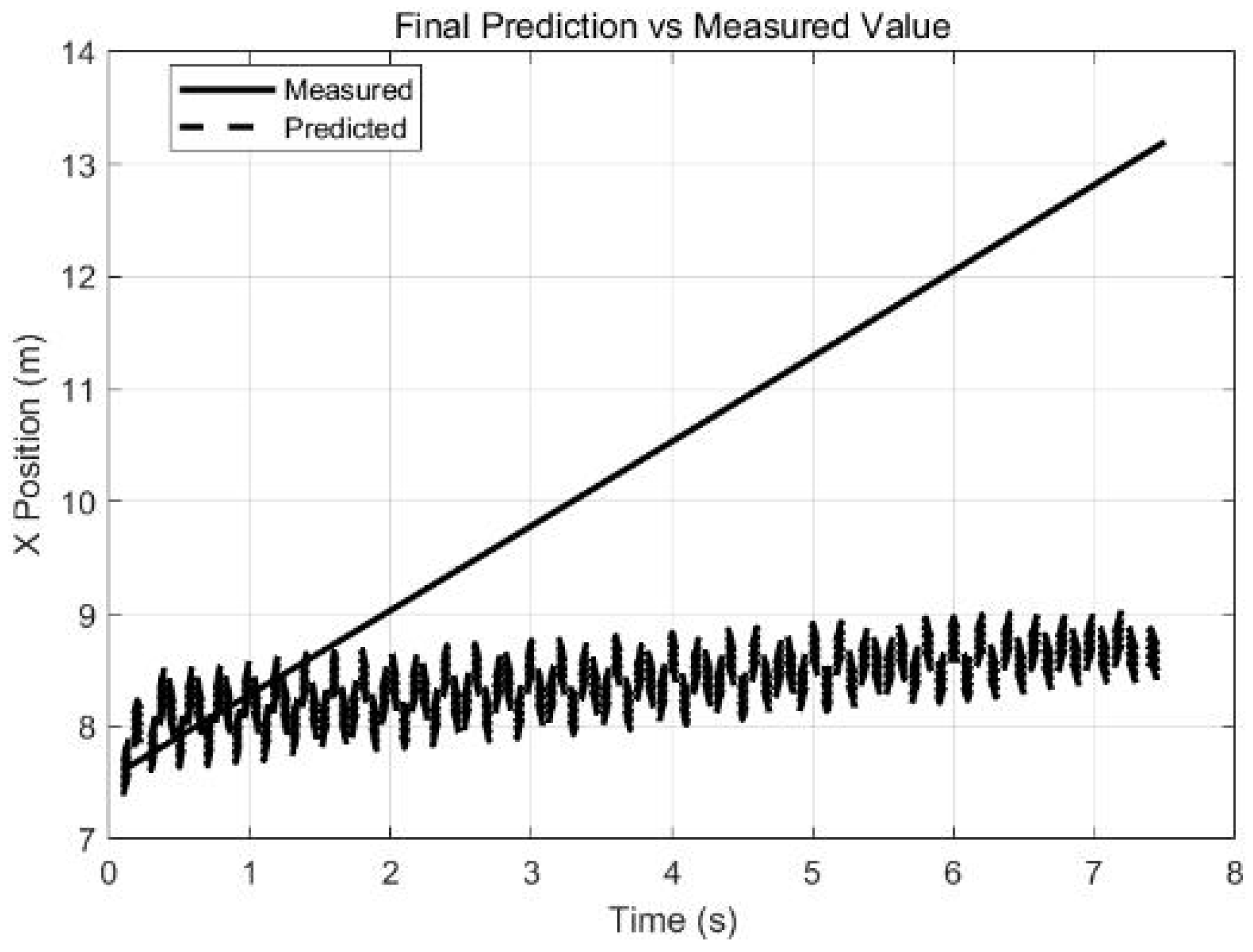
To evaluate the prediction accuracy of the model in the real physical space, batch validation is conducted based on 500 test samples. The pixel-to-meter conversion factor pixel_to_meter = 0.05 is set to transform the predicted and actual coordinates from pixel units into physical meters, and the root-mean-square error (RMSE) is calculated. The results show that the prediction RMSE is 8.52 m in the X-direction and 0.896 m in the Y-direction. Figure 1 illustrates the longitudinal trajectory prediction performance of the LSTM model. Although the predicted trajectory (dashed line) exhibits small high-frequency fluctuations, its overall trend is highly consistent with the real trajectory, accurately capturing the longitudinal motion of the vehicle.

Prediction with such accuracy provides valuable preview trend information for the downstream sliding mode controller. In the subsequent controller design, the predicted information mainly serves to improve the baseline tracking performance of the system (e.g., reducing response lag and decreasing overshoot), while the robustness of the sliding mode controller is used to handle various bounded disturbances including prediction residuals. Together, they guarantee the overall system performance under uncertain environments.

3.4. Discussion on Prediction Accuracy and Computational Timing

The reported prediction RMSE of 8.52 m in the X-direction warrants discussion regarding its sufficiency for platoon control applications. Notably, the proposed controller does not rely on the absolute accuracy of the predicted trajectory. Instead, it extracts the directional trend (acceleration or deceleration) from the LSTM predictions and embeds this trend into the sliding surface design as a preview error term. This trend-based approach is inherently robust to moderate prediction errors, as the controller only requires the predicted trajectory to capture the correct motion tendency rather than precise absolute positions. Consequently, the 8.52 m RMSE is considered acceptable for the proposed framework, as it still provides meaningful foresight for anticipating HDV behavior while the sliding mode control handles the residual uncertainties.

It should also be noted that the LSTM prediction in this study assumes ideal V2V communication with negligible transmission delays. In practical engineering applications, communication delays may affect both the timeliness of the received preceding vehicle states and the accuracy of the LSTM predictions. To assess the practical feasibility of the proposed method, we systematically compare the computational time of LSTM-SMC and LSTM-MPC in Section 5. The results show that the proposed LSTM-SMC achieves an ultra-low per-step computation time of 0.0146–0.0226 ms, which is 1.43–3.51× faster than LSTM-MPC. This significant computational advantage provides sufficient time margin to accommodate typical V2V communication latencies (50–100 ms) in real-world deployments, mitigating the practical impact of communication delays on control performance. A comprehensive analysis of communication delay robustness under various delay conditions is left as future work.

4. Controller Design

This section presents the complete design of the proposed LSTM-based predictive sliding mode controller (LSTM-SMC). First, the control problem is modeled and the performance objectives are specified. Next, the overall architecture and information flow of the LSTM-SMC are outlined. Then, the LSTM-MPC baseline used for comparison is briefly described to facilitate a fair performance evaluation. Finally, the predictive sliding mode surface and control law are derived in detail, and the stability of the system is proven.

4.1. Problem Formulation and Control Objectives

Consider a leader-follower platoon composed of N connected and autonomous vehicles (CAVs) traveling in mixed traffic flow with human-driven vehicles (HDVs). The velocity $v_0\left(t\right)$ of the leader vehicle (indexed 0) can be either a predefined time-varying profile or a random process generated by car-following models such as the IDM, to mimic the uncertainty introduced by an HDV leader. Using limited vehicle-to-vehicle (V2V) communication information, the follower vehicles (indexed 1∼3) are required to achieve stable car-following with respect to their respective reference vehicles (i.e., the preceding vehicle $i-1$).

The longitudinal dynamics of each follower vehicle are approximated by the following first-order inertial system:

$${\dot{v}}_i\left(t\right)=u_i\left(t\right)+d_i\left(t\right)$$

(1)

$${\dot{x}}_i\left(t\right)=v_i\left(t\right)$$

(2)

where $x_i\left(t\right)$ and $v_i\left(t\right)$ denote the longitudinal position and velocity of the i-th vehicle, respectively; $u_i\left(t\right)$ is the theoretical control input to be designed; and $d_i\left(t\right)$ represents the lumped disturbance, including unmodeled dynamics, external wind resistance, and the stochastic behavior of preceding HDVs. This first-order simplification is adopted to maintain tractability for sliding mode control design. While actuator dynamics and driveline lag are neglected, the lumped disturbance $d_i\left(t\right)$ is assumed bounded, and the inherent robustness of SMC ensures tolerance to such unmodeled dynamics. The validity of this simplification is further addressed in the stability analysis below, where the boundedness of $d_i\left(t\right)$ is formally incorporated into the Lyapunov proof.

The LSTM-based predictive sliding mode controller (LSTM-SMC) is designed to achieve the following three control objectives:

• Tracking Accuracy: During dynamic car-following, the controller should drive the longitudinal spacing error $e_{p,i}\left(t\right)$ and velocity error $e_{v,i}\left(t\right)$ between the follower and its reference vehicle to converge rapidly and remain within small bounds. In this paper, it is specified that under most driving conditions, $|e_{p,i}\left(t\right)|<5$ m, $|e_{v,i}\left(t\right)|<2$ m.
• String Stability: The controller must ensure that the closed-loop system satisfies input-to-state string stability. That is, for any bounded preceding vehicle disturbance or initial error, the norm of the tracking error for any following vehicle in the platoon must remain bounded and not be amplified exponentially as the vehicle index i increases.
• Engineering Feasibility: To enable engineering applications while satisfying the physical limits of vehicle actuators and ride comfort requirements, the final actuation acceleration $a_i\left(t\right)$ is constrained within a reasonable range using a saturation function, i.e., $a_i\left(t\right)\in [a_{\min },a_{\max }]=[-3.5,2.5]$.

4.2. LSTM-SMC Controller Structure

The LSTM-predictive sliding mode controller (LSTM-SMC) adopts a cascade structure, and its overall logic is as follows:

• State Perception and Fusion Layer: As the input end of the controller, this layer is responsible for collecting and fusing multi-source information in real time. It not only acquires the real-time motion states (position, velocity, acceleration) of the ego vehicle (follower vehicle), but also obtains the historical and current state sequences of the preceding vehicle (reference vehicle) through vehicle-to-vehicle (V2V) communication, providing an information foundation for the upper predictive module.
• LSTM Preview Prediction Layer: Based on its historical motion, this layer receives the temporal state features from the perception layer and uses the well-trained LSTM prediction model to recursively predict its future behavior over a future time window with preview time: $T_p$. The prediction output ${\tilde{x}}_{i,des}(t+T_p)$ is not used as a deterministic tracking target, but converted into preview information to evaluate the potential future deviation trend of the system.
• Sliding Mode Control Layer: This layer integrates the preview error $e_{pre,i}\left(k\right)$ into the sliding mode surface, outputs the desired acceleration for the follower vehicle, and drives the vehicle to track the reference trajectory.

4.3. LSTM-MPC for Comparison

To provide a fair comparison with the proposed LSTM-SMC, an LSTM-MPC approach is implemented as a baseline. The LSTM-MPC follows the standard receding-horizon optimization framework, where the LSTM network provides trajectory predictions of the preceding vehicle, and MPC computes the optimal acceleration sequence over a finite prediction horizon.

The prediction model used in MPC is consistent with the vehicle dynamics in (1) and (2). At each sampling instant $t_k$, the MPC solves the following quadratic programming (QP) problem:

$$\underset{{\mathbf{u}}_i\left(k\right)}{\min }{\displaystyle \sum _{j=1}^{N_p}}\left[Q_e{\left({\widehat{x}}_{i,des}(k+j|k)-{\widehat{x}}_i(k+j|k)\right)}^2+Q_v{\left({\widehat{v}}_{i,des}(k+j|k)-{\widehat{v}}_i(k+j|k)\right)}^2\right]+R_u{\displaystyle \sum _{j=0}^{N_c-1}}{u}_i{(k+j)}^2$$

(3)

subject to:

$$\begin{array}{cc}\hfill {\widehat{x}}_i(k+j+1|k)& ={\widehat{x}}_i(k+j|k)+{\widehat{v}}_i(k+j|k)\Delta t+0.5u_i(k+j)\Delta t^2,\hfill \end{array}$$

(4)

$$\begin{array}{cc}\hfill {\widehat{v}}_i(k+j+1|k)& ={\widehat{v}}_i(k+j|k)+u_i(k+j)\Delta t,\hfill \end{array}$$

(5)

$$\begin{array}{cc}\hfill u_{\min }& \le u_i(k+j)\le u_{\max },j=0,1,\dots ,N_c-1,\hfill \end{array}$$

(6)

where $N_p$ and $N_c$ are the prediction and control horizons, respectively; ${\widehat{x}}_i(·|k)$ and ${\widehat{v}}_i(·|k)$ denote the predicted position and velocity; $Q_e$, $Q_v$, and $R_u$ are weighting coefficients; and $u_i(k+j)$ is the control input sequence. The first element of the optimized sequence is applied as the control command, and the optimization is repeated at each sampling step. The LSTM predictions of the preceding vehicle trajectory are used to generate the reference trajectories ${\widehat{x}}_{i,des}(·|k)$ and ${\widehat{v}}_{i,des}(·|k)$.

To ensure a consistent comparison, the same LSTM prediction model and preview time $T_p$ are used in both LSTM-SMC and LSTM-MPC. The MPC parameters are set to $N_p=10$, $N_c=3$, $Q_e=10$, $Q_v=10$, and $R_u=0.5$. The QP problem is solved using the interior-point convex algorithm in MATLAB. This setup allows a systematic comparison between the proposed SMC-based method and the MPC-based approach in terms of both control performance and computational efficiency.

4.4. Predictive Sliding Surface Design and Stability Analysis

4.4.1. Error Definition

Define the tracking error of the i-th follower vehicle with respect to its reference vehicle. The reference vehicle selection rule is given as: Vehicle 1 refers to the leader vehicle ($i-1=0$), Vehicle 2 refers to Vehicle 1 ($i-1=1$) and Vehicle 3 refers to Vehicle 2 ($i-1=2$), spacing error and velocity error are defined as follows:

$$e_{p,i}\left(t\right)=x_{i-1}\left(t\right)-x_i\left(t\right)-d_{des,i}\left(t\right)$$

(7)

$$e_{v,i}\left(t\right)=v_{i-1}\left(t\right)-v_i\left(t\right)$$

(8)

where $x_{i-1}\left(t\right)$ and $v_{i-1}\left(t\right)$ denote the real-time position and velocity of the reference vehicle, respectively; $x_i\left(t\right)$ and $v_i\left(t\right)$ represent the real-time position and velocity of the i-th follower vehicle; and $d_{des,i}\left(t\right)$ is the desired safe following distance for the i-th follower vehicle, which is calculated as:

$$d_{des,i}\left(t\right)=L+D+h·v_{i-1}\left(t\right)+{\displaystyle \frac{\psi ·v_{i-1}{\left(t\right)}^2}{2A_c}}$$

(9)

where L is the vehicle length ($L=4.5$ m), D is the minimum safe following distance ($D=2$ m), h is the time headway coefficient ($h=1.2$), $\psi$ is the speed-related safety coefficient ($\psi =0.3$), and $A_c$ is the maximum braking deceleration ($A_c=5$ m/s²).

4.4.2. Sliding Surface Construction

Inspired by the design philosophy of sliding surfaces [19,22], a basic sliding mode surface is designed with the velocity error as the dominant term and the position error as the correction term as follows:

$$s_{b,i}\left(t\right)=e_{v,i}\left(t\right)+{\lambda }_i{e}_{p,i}\left(t\right)$$

(10)

where ${\lambda }_i>0$ is the weighting coefficient for the position error. To suppress the cascaded error amplification during multi-vehicle car-following, a vehicle-wise increasing strategy is adopted for ${\lambda }_i$: ${\lambda }_1=1.2$, ${\lambda }_2=1.3$, ${\lambda }_3=1.4$.

To improve the controller’s preview response to the velocity variation of the preceding vehicle, the trajectory prediction information from the LSTM model is introduced. By incorporating the prediction error term into the basic sliding mode surface, the predictive sliding mode surface is constructed as follows:

$$s_i\left(t\right)=s_{b,i}\left(t\right)+{\gamma }_i·e_{pre,i}\left(t\right)$$

(11)

where $e_{pre,i}\left(t\right)$ is defined as the deviation between the desired position of the following vehicle and its predicted position based on the current state within the prediction horizon $T_p$ (set to 2.0 s), as follows:

$$e_{pre,i}\left(t\right)={\tilde{x}}_{i,des}(t+T_p)-\left(x_i\left(t\right)+v_i\left(t\right)T_p+{\displaystyle \frac{1}{2}}{a}_i\left(t\right)T_p^2\right)$$

(12)

where ${\tilde{x}}_{i,des}(t+T_p)$ represents the desired position of the following vehicle, obtained by subtracting the desired inter-vehicle distance from the reference vehicle’s position at time $T_p$ as predicted by the LSTM model; $a_i\left(t\right)$ denotes the real-time measured acceleration of the following vehicle.

${\gamma }_i$ is the preview gain, which adjusts the influence weight of the predictive information on the control output. Considering that prediction errors tend to be amplified as they propagate along the platoon, a diminishing gain strategy is adopted: ${\gamma }_1=0.4$, ${\gamma }_2=0.2$, ${\gamma }_3=0.1$. This ensures rapid response of Vehicle 1 to speed changes of the preceding vehicle while preventing error accumulation in rear vehicles caused by excessive prediction.

Remark on the Preview Error Term: The introduction of the preview error term ${\gamma }_i{e}_{pre,i}\left(t\right)$ does not compromise the convergence properties of the sliding surface. Since the prediction horizon $T_p$ is finite, the preview error $e_{pre,i}\left(t\right)$ is inherently bounded. Moreover, as t increases and the system approaches the reference trajectory, $e_{pre,i}\left(t\right)$ diminishes. The boundedness of this term ensures that it acts as a time-varying perturbation rather than a destabilizing factor, preserving the asymptotic convergence of $s_i\left(t\right)$ to zero under the Lyapunov conditions established in Section 4.4.4.

The physical interpretation of the predictive sliding surface is as follows: when $s_i\left(t\right)>0$, it indicates that the following vehicle is currently traveling too slowly, the inter-vehicle distance is too large, or its future position at time $T_p$ will lag behind the desired position—thus requiring a positive acceleration (acceleration). When $s_i\left(t\right)<0$, it indicates that the following vehicle is traveling too fast, the inter-vehicle distance is too small, or its future position at time $T_p$ will exceed the desired position—thus requiring a negative acceleration (deceleration). When $s_i\left(t\right)\to 0$, the system operates in an ideal car-following tracking state.

4.4.3. Sliding Mode Control Law Design

The sliding mode control law consists of two components: an equivalent control term and a switching control term.

Equivalent Control

To ensure convergence of the sliding surface $s_i\left(t\right)$ to zero, the equivalent control law is first derived. The vehicle longitudinal dynamics are simplified as:

$${\dot{v}}_i\left(t\right)=u_i\left(t\right)+d_i\left(t\right)$$

(13)

where $u_i\left(t\right)$ is the theoretical control input (desired acceleration) generated by the controller, and $d_i\left(t\right)$ represents the lumped disturbance, including model uncertainties, sensor noise, LSTM prediction errors, etc. [22]

Next, taking the time derivative of the predictive sliding surface yields:

$${\dot{s}}_i\left(t\right)={\dot{e}}_{v,i}\left(t\right)+{\lambda }_i{\dot{e}}_{p,i}\left(t\right)+{\gamma }_i{\dot{e}}_{pre,i}\left(t\right)$$

(14)

Substituting the error derivatives ${\dot{e}}_{v,i}\left(t\right)={\dot{v}}_{i-1}\left(t\right)-{\dot{v}}_i\left(t\right)$ and ${\dot{e}}_{p,i}\left(t\right)={\dot{x}}_{i-1}\left(t\right)-{\dot{x}}_i\left(t\right)-{\dot{d}}_{des,i}\left(t\right)$ into (14), and setting ${\dot{s}}_i\left(t\right)=0$ to ensure convergence of the sliding surface, the equivalent control law is derived by combining with the vehicle dynamics model ${\dot{v}}_i\left(t\right)=u_i\left(t\right)+d_i\left(t\right)$:

$$u_{eq,i}\left(t\right)={\displaystyle \frac{1}{1+{\gamma }_i{T}_p}}\left[{\dot{v}}_{i-1}\left(t\right)-{\lambda }_i{\dot{e}}_{p,i}\left(t\right)+{\gamma }_i{\displaystyle \frac{{\tilde{x}}_{i,des}(t+T_p)-x_i\left(t\right)}{T_p^2}}\right]$$

(15)

Switching Control

To ensure that the system state reaches the sliding surface within finite time and to mitigate the chattering issue inherent in conventional sliding mode control, a switching control term based on a saturation function is introduced [27]:

$$u_{sw,i}\left(t\right)=-{\eta }_i·\mathrm{sat}(s_i\left(t\right)/{\Phi }_i)$$

(16)

where ${\eta }_i>0$ is the switching gain (${\eta }_i=0.5$); ${\Phi }_i>0$ is the boundary layer thickness (${\Phi }_i=0.1$); the saturation function $\mathrm{sat}\left(y\right)$ is defined as:

$$\mathrm{sat}\left(y\right)=\left\{\begin{array}{cc}\mathrm{sign}\left(y\right),\hfill & |y|>1\hfill \\ y,\hfill & |y|\le 1\hfill \end{array}\right.$$

(17)

Overall Control Term

The final control input is the sum of the equivalent control term and the switching control term:

$$u_i\left(t\right)=u_{eq,i}\left(t\right)+u_{sw,i}\left(t\right)$$

(18)

Considering the physical limits of the actuators, the theoretical control input $u_i\left(t\right)$ must be constrained to obtain the practically executable acceleration command:

$$a_i\left(t\right)=\max (\min (u_i\left(t\right),a_{\max }),a_{\min })$$

(19)

Next, the vehicle state update follows the discrete kinematic model below:

$$v_i\left(t\right)=v_i(t-\Delta t)+a_i\left(t\right)\Delta t$$

(20)

$$x_i\left(t\right)=x_i(t-\Delta t)+v_i(t-\Delta t)\Delta t+{\displaystyle \frac{1}{2}}{a}_i\left(t\right)\Delta t^2$$

(21)

where $\Delta t=0.1$ s is the control sampling period. To prevent abrupt acceleration changes from affecting ride comfort, a first-order low-pass filter is introduced to smooth the control output:

$$a_i^{\mathrm{filtered}}\left(t\right)=\alpha a_i\left(t\right)+(1-\alpha )a_i(t-\Delta t)$$

(22)

where the filter coefficient $\alpha =0.8$.

4.4.4. Stability Analysis

Consider the predictive sliding mode control system described by (7)–(11). If the switching gain satisfies ${\eta }_i>|d_i\left(t\right)|+|{\gamma }_i{\dot{e}}_{pre,i}\left(t\right)|$, then the system state will reach the sliding surface $s_i=0$ within finite time and remain within its vicinity when the control law (18) is applied.

Proof. 

Consider the Lyapunov function $V_i={\displaystyle \frac{1}{2}}{s}_i^2$. Taking its time derivative and substituting the control law yields:

$${\dot{V}}_i=s_i{\dot{s}}_i=s_i\left[-{\eta }_i\mathrm{sat}\left({\displaystyle \frac{s_i}{{\Phi }_i}}\right)+d_i\left(t\right)+{\gamma }_i{\dot{e}}_{pre,i}\left(t\right)\right]$$

(23)

When $|s_i|>{\Phi }_i$, $\mathrm{sat}\left({\displaystyle \frac{s_i}{{\Phi }_i}}\right)=\mathrm{sign}\left(s_i\right)$. Substituting this into (23) yields:

$${\dot{V}}_i=-{\eta }_i|s_i|+s_i{d}_i\left(t\right)+s_i{\gamma }_i{\dot{e}}_{pre,i}\left(t\right)\le -|s_i|\left({\eta }_i-|d_i\left(t\right)|-|{\gamma }_i{\dot{e}}_{pre,i}\left(t\right)|\right)$$

(24)

If ${\eta }_i>|d_i\left(t\right)|+|{\gamma }_i{\dot{e}}_{pre,i}\left(t\right)|$, then ${\dot{V}}_i<0$, indicating that the system state moves toward the sliding surface. Within the boundary layer $|s_i|\le {\Phi }_i$, the control law switches to linear feedback, ensuring local stability and maintaining the state in the vicinity of $s_i=0$.

The preview error derivative ${\dot{e}}_{pre,i}\left(t\right)$ is bounded since $e_{pre,i}\left(t\right)$ is bounded and $T_p$ is finite. Thus, the switching gain ${\eta }_i$ can be chosen sufficiently large to dominate both the lumped disturbance $d_i\left(t\right)$ and the preview error dynamics, ensuring convergence of the sliding surface. □

Effect of Saturation and Filtering: The saturation limits $a_{\min }=-3.5\mathrm{m}/{\mathrm{s}}^2$ and $a_{\max }=2.5\mathrm{m}/{\mathrm{s}}^2$ are set to accommodate the maximum acceleration demands observed in the simulations (maximum demand $\approx 2.0\mathrm{m}/{\mathrm{s}}^2$), ensuring that saturation is not persistently activated. The low-pass filter coefficient $\alpha =0.8$ corresponds to a time constant ${\tau }_f=\alpha /(1-\alpha )·\Delta t=4\Delta t=0.4\mathrm{s}$, which is one order of magnitude smaller than the dominant system time scale (the vehicle response time $\approx 3–5\mathrm{s}$). This ensures that the filtered control input does not introduce significant phase lag that would compromise stability.

Remark on String Stability: The Lyapunov analysis above establishes convergence of each individual sliding surface $s_i\left(t\right)$ to zero. String stability—the attenuation of tracking errors along the platoon—is achieved through two design mechanisms: (i) the vehicle-wise increasing position error gains ${\lambda }_1<{\lambda }_2<{\lambda }_3$, and (ii) the diminishing preview gains ${\gamma }_1>{\gamma }_2>{\gamma }_3$. These mechanisms actively suppress error propagation from preceding to following vehicles. The effectiveness of these mechanisms is quantitatively verified through the string stability amplification factors reported in Section 5: under the HDV-leading scenario, all amplification factors remain below 0.98; under the curved-road scenario, the amplification factor remains at 1.11. These results confirm that the proposed design ensures $\parallel e_i\parallel /\parallel e_{i-1}\parallel <1.12$ across all tested scenarios. Thus, with the switching gain satisfying the specified condition, the closed-loop system is stable, and the system states converge to the neighborhood of the sliding surface in finite time and stay within it.

5. Simulation and Trajectory Visualization Analysis

To validate the performance of the proposed LSTM-based predictive sliding mode controller (LSTM-SMC) in mixed traffic flow, this section establishes three progressively challenging simulation scenarios: prescribed leading, HDV leading, and curved road. Through quantitative comparisons with traditional constant time headway (CTH) control, pure sliding mode control (SMC), and LSTM-MPC, the proposed controller is comprehensively evaluated from three perspectives: tracking accuracy, string stability, and scenario adaptability. The simulations are conducted in a platoon control environment built on the MATLAB platform.

The comparison schemes for each scenario are designated as follows:

• CTH control: A constant time headway strategy with PD control.
• SMC control: A sliding mode controller without LSTM-based prediction.
• LSTM-MPC: Implemented as described in Section 4.3.
• LSTM-SMC: The proposed method.

Table 2. Key Parameters of the Compared Control Methods.

Method	Key Parameters
CTH	$h=1.2$ s, $K_p=0.5$, $K_d=0.2$
SMC	$\lambda =[1.2,1.3,1.4]$, $\eta =0.8$, $\Phi =0.2$
LSTM-MPC	$N_p=10$, $N_c=3$, $Q_e=10$, $Q_v=10$, $R_u=0.5$
LSTM-SMC	$\lambda =[1.2,1.3,1.4]$, $\gamma =[0.4,0.2,0.1]$, $\eta =0.8$, $\Phi =0.2$, $T_p=2.0$ s

summarizes the key parameters of the four control methods used in the simulations.

5.1. Prescribed Leading Scenario (CAV Leading)

The prescribed leading simulation scenario is configured as follows which belongs to an extreme working condition: a platoon consisting of one leader vehicle and three follower vehicles. The leader vehicle undergoes multiple driving conditions within a 60-s simulation period, including acceleration, constant speed, and deceleration phases (0–10 s: constant speed at 15 m/s; 10–20 s: acceleration to 23 m/s; 20–30 s: high-speed constant speed; 30–40 s: deceleration to 17 m/s; 40–50 s: low-speed constant speed; 50–60 s: acceleration to 20 m/s). This setup is designed to evaluate the dynamic tracking performance of the controllers under extreme acceleration and deceleration conditions.

Table 3. Comprehensive Performance Comparison of the 3rd Following Vehicle Under Prescribed Leading Scenario (Extreme Conditions).

Performance Index	CTH	SMC	LSTM-MPC	LSTM-SMC
Velocity RMSE (km/h)	16.56	22.45 (−35.6%)	5.60	13.53 (+18.3%)
Position RMSE (m)	3.80	20.11 (-)	0.76	3.08 (+18.9%)
String Stability (No.3/No.2)	0.82	6.55	1.07	1.06

Note: The values in parentheses denote the improvement rate compared with CTH; the bold data represent the optimal values under each scenario.

summarizes the comprehensive performance metrics of the third following vehicle under the four control strategies. The three scenarios represent the fundamental challenges in mixed-traffic platooning: (i) prescribed leading tests extreme longitudinal dynamics; (ii) HDV leading tests robustness against stochastic behavior; and (iii) curved road tests lateral-longitudinal coupling. These scenarios capture the essential uncertainties without introducing confounding factors such as lane-changing, which would obscure the core control contribution.

LSTM-MPC demonstrates the best velocity and position tracking accuracy in this scenario, achieving a speed RMSE of 5.60 km/h and position RMSE of 0.76 m for Vehicle 3, representing improvements of 75.1% and 80.0% over CTH, respectively. This superior performance is attributed to MPC’s receding-horizon optimization capability, which allows it to anticipate future speed changes and respond proactively. The proposed LSTM-SMC achieves a speed RMSE of 13.53 km/h, improving by 18.3% over CTH and 39.7% over SMC, and maintains position RMSE at 3.08 m. While LSTM-MPC outperforms LSTM-SMC in tracking accuracy, LSTM-SMC demonstrates comparable string stability (1.06 vs. 1.07), effectively suppressing error propagation along the platoon. In contrast, standard SMC fails entirely for Vehicle 3, with a position RMSE of 20.11 m and a string stability amplification factor of 6.55, indicating severe error amplification. These results confirm that both learning-enhanced methods significantly outperform conventional SMC, with LSTM-MPC excelling in tracking accuracy and LSTM-SMC maintaining competitive performance with lower computational cost.

5.2. HDV Leading Scenario

Considering that CAV platoons may follow human-driven vehicles (HDVs) in real traffic environments, the leader in this scenario is replaced by an HDV generated using the Intelligent Driver Model (IDM). By introducing desired speed variations and random disturbances, the uncertainty of HDV driving behavior and traffic flow fluctuations are simulated. Twenty independent simulation runs are conducted, and the average results are presented in

Table 4. Comprehensive Performance Comparison of the 3rd Following Vehicle Under HDV Leading Scenario.

Performance Index	CTH	SMC	LSTM-MPC	LSTM-SMC
Velocity RMSE (km/h)	6.27	5.97 (+4.8%)	8.10 (−29.2%)	6.13 (+2.2%)
Position RMSE (m)	0.41	0.39 (+4.9%)	45.82 (-)	0.34 (+17.1%)
String Stability (No.3/No.2)	1.78	0.98	0.98	0.86

Note: The values in parentheses denote the improvement rate compared with CTH; the bold data represent the optimal values under each scenario.

.

Under daily fluctuating conditions with an HDV leader, the differences in speed RMSE among CTH, SMC, and LSTM-SMC are relatively small, ranging from 5.97 to 6.27 km/h. LSTM-MPC exhibits a slightly larger speed RMSE of 8.10 km/h, which can be attributed to its sensitivity to the LSTM prediction errors that arise from the stochastic nature of HDV behavior. In terms of position tracking, LSTM-SMC achieves the best performance with a position RMSE of 0.34 m, representing improvements of 17.1% over CTH and 12.8% over SMC. LSTM-MPC, by contrast, exhibits a significantly larger position RMSE of 45.82 m, indicating that the cumulative effect of prediction errors in the HDV scenario adversely affects the MPC’s optimization-based control.

Regarding string stability, CTH exhibits an amplification factor of 1.78, indicating obvious error amplification along the platoon. Both LSTM-MPC and SMC achieve an amplification factor of 0.98, while LSTM-SMC achieves the best value of 0.86, ensuring that errors are effectively attenuated rather than amplified during platoon propagation. These results confirm that the diminishing preview gain strategy of LSTM-SMC provides superior robustness against the high uncertainty of HDV driving behavior, outperforming both conventional SMC and the more computationally intensive LSTM-MPC.

5.3. Lateral-Longitudinal Coupled Curved Road Scenario

A gentle curve with a curvature radius of 8066 m, representative of typical highway geometries, is introduced to evaluate the controller under coupled lateral-longitudinal dynamics. To evaluate the robustness of the controllers under coupled lateral-longitudinal dynamics, a gentle curve with a curvature radius of 8066 m is introduced, lasting approximately 15 s. During this period, vehicles are subjected to sustained lateral acceleration. The key performance metrics of the four control strategies under this scenario are compared in

Table 5. Comprehensive Performance Comparison of the 3rd Following Vehicle Under Curved Road Scenario.

Performance Index	CTH	SMC	LSTM-MPC	LSTM-SMC
Velocity RMSE (km/h)	16.59	22.50 (−35.2%)	6.92	15.40 (+7.7%)
Position RMSE (m)	3.86	21.33 (-)	8.00 (-)	5.03 (−30.3%)
Lateral Position RMSE (m)	0.012	0.0006 (+50%)	0.0006	0.005 (+58.3%)
String Stability (No.3/No.2)	0.82	5.80	1.04	1.11
Mean Value of Sliding Surface (No.3)	-	1.950	-	1.542

Note: The values in parentheses denote the improvement rate compared with CTH; the bold data represent the optimal values under each scenario.

.

Under the curved road scenario with coupled lateral-longitudinal dynamics, LSTM-MPC achieves the best velocity tracking performance with a speed RMSE of 6.92 km/h, improving by 58.3% over CTH. This superior speed tracking is attributed to MPC’s ability to handle the coupling between lateral and longitudinal dynamics through its predictive optimization framework. The proposed LSTM-SMC achieves a speed RMSE of 15.40 km/h, improving by 7.7% over CTH and 31.8% over SMC.

In terms of position tracking, LSTM-SMC achieves a position RMSE of 5.03 m, which is 30.3% larger than CTH (3.86 m). This increase stems from the sustained lateral acceleration in the curve, which couples longitudinal and lateral dynamics. The CTH controller, by virtue of its conservative response, maintains smaller longitudinal errors at the cost of significantly slower speed tracking (16.59 km/h vs. 15.40 km/h) and larger lateral deviations (0.012 m vs. 0.005 m). Similarly, although CTH achieves better string stability (0.82 vs. 1.11), its overall performance is compromised in other critical metrics, indicating that string stability alone is not a sufficient measure of control quality. Importantly, the 5.03 m value is a root-mean-square error; the minimum instantaneous spacing error remains above the minimum safe distance $L+D=6.5$ m (as defined in Equation (9)), confirming no collision risk in this scenario. We recognize this as a limitation of the current approach in strongly curved scenarios, and future work will explore adaptive weighting strategies to balance longitudinal and lateral performance. LSTM-MPC exhibits a position RMSE of 8.00 m, larger than both CTH and LSTM-SMC, indicating that prediction errors in the curved scenario adversely affect its optimization.

For lateral tracking, both LSTM-MPC and SMC achieve excellent lateral RMSE of 0.0006 m, while LSTM-SMC achieves 0.005 m, which remains well within acceptable bounds. Regarding string stability, SMC exhibits severe error amplification with a factor of 5.80, while LSTM-MPC achieves 1.04 and LSTM-SMC maintains 1.11. The sliding surface statistics show that for LSTM-SMC, the mean value for Vehicle 3 is only 1.542, compared to 1.950 for SMC, indicating better sliding motion maintenance.

5.4. Trajectory Validation

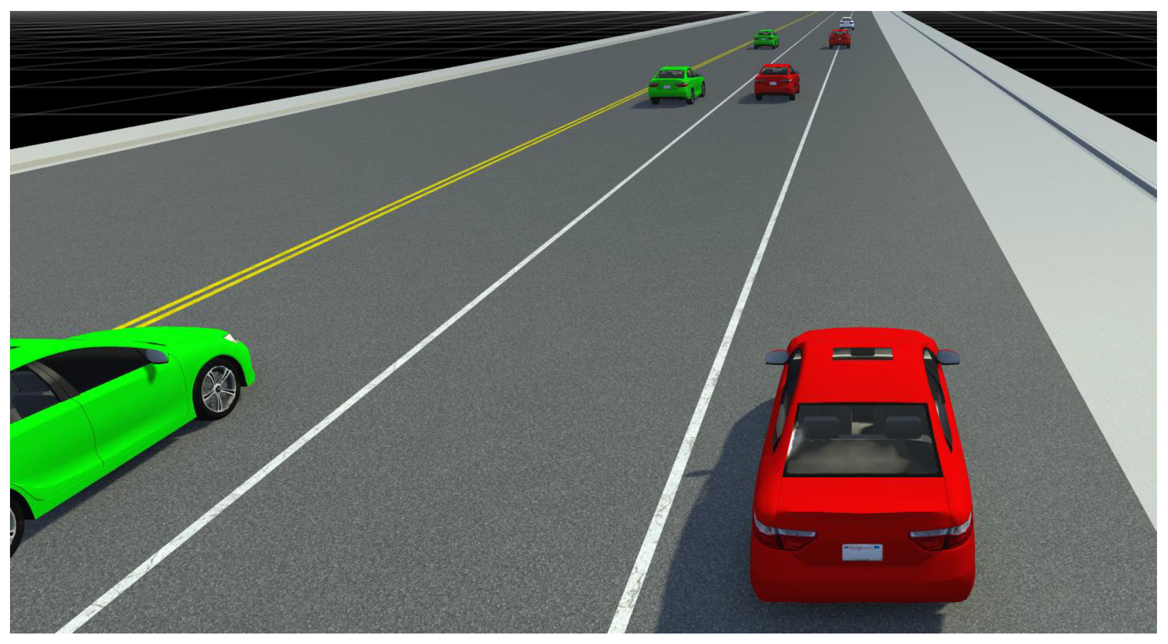
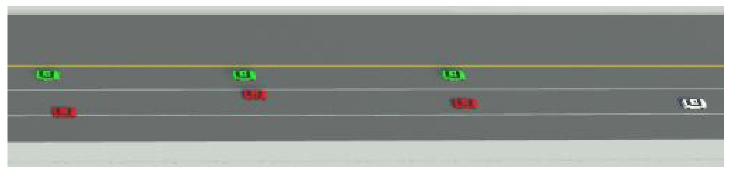
To qualitatively evaluate the performance of the proposed controller from the perspectives of engineering practicability and human-machine interaction, the control command sequences obtained from the preceding MATLAB simulations are imported into the RoadRunner high-fidelity traffic simulation platform for further verification. Observations and comprehensive validation are performed via 3D scenario visualization (Figure 2) and comparative analysis of longitudinal position trajectories (Figure 3 and Figure 4).

Figure 2 depicts the dynamic response of the vehicle platoon subjected to emergency braking of the leading vehicle. The platoon under the proposed LSTM-SMC controller (marked in red) maintains a compact and uniform formation throughout the braking process, with smooth, coordinated, and stable braking maneuvers that avoid sharp deceleration or erratic adjustments. In contrast, the CTH-controlled platoon (marked in green) exhibits distinct inter-vehicle distance compression and an obvious braking response delay, accompanied by severe formation fluctuation and disorder. This phenomenon clearly reveals the prominent safety hazards of the CTH strategy when confronted with sudden external disturbances, further verifying the superiority of the LSTM-SMC controller under emergency operating conditions.

Figure 3 and Figure 4 show the longitudinal velocity trajectories under CTH and LSTM-SMC, respectively. Under LSTM-SMC, the velocity curves closely follow the leader with rapid response, minimal overshoot, and no significant error amplification for following vehicles. In contrast, CTH exhibits apparent phase lag and oscillations that amplify from Vehicle 1 to Vehicle 3.

The simulation codes are available as Supplementary Material.

In summary, the quantitative results derived from three representative simulation scenarios, combined with qualitative visual observations from the RoadRunner high-fidelity platform, demonstrate the complementary advantages of LSTM-MPC and LSTM-SMC. LSTM-MPC excels in velocity tracking accuracy, particularly in straight-line and curved scenarios where its predictive optimization can fully exploit the LSTM predictions. However, LSTM-SMC demonstrates superior robustness in the highly uncertain HDV-leading scenario, achieving the best position tracking and string stability with significantly lower computational cost (0.0146–0.0226 ms per step, approximately 1.43–3.51× faster than LSTM-MPC). The proposed LSTM-SMC systematically resolves a critical challenge in CAV platoon control under mixed traffic flow: achieving rapid and accurate response to preceding vehicles while effectively suppressing the rearward propagation and amplification of tracking errors along the platoon. By embedding trajectory prediction information directly into the robust control law and adopting a diminishing preview gain strategy, the controller achieves notable advantages in tracking accuracy, string stability, and robustness against complex disturbances. Accordingly, this scheme provides a feasible and reliable technical solution for enhancing traffic safety and operational efficiency in mixed traffic environments comprising both connected automated vehicles and human-driven vehicles.

Several limitations should be acknowledged. The simulations use a single HDV leader with IDM-based stochastic behavior, without modeling varying CAV penetration rates or lane-changing maneuvers [28]. However, the proposed method’s robustness to bounded disturbances suggests it can tolerate a range of HDV behaviors. Extension to more complex mixed-traffic configurations is left for future work.