Radar-Camera Extrinsic Calibration for Roadside Infrastructure: A Systematic Review

Abstract

The growth of Intelligent Transportation Systems (ITS) has made high-quality perception data from multi-sensor setups essential. Pairing millimeter-wave (mmW) radar with a monocular camera is a common way to recover three-dimensional information about the environment, but aligning the two is difficult because sparse radar point clouds and dense camera images differ sharply in how they sense a scene. The problem grows more severe in roadside infrastructure, where the high mounting elevation introduces perspective distortion that vehicle-mounted systems rarely face. This paper presents a systematic review, conducted under the Preferred Reporting Items for Systematic Reviews and Meta-Analyses (PRISMA) guidelines, of radar-camera extrinsic calibration for fixed roadside infrastructure, organizing existing work into a taxonomy that separates traditional two-stage pipelines from recent end-to-end learning frameworks. Because methods designed specifically for roadside units remain scarce, the review also covers vehicle- and robot-mounted methods whose static-sensor formulation carries over to fixed roadside deployment. For the two-stage pipeline, the analysis covers target-based and targetless correspondence registration along with the optimization techniques and algorithmic assumptions behind parameter estimation. The end-to-end learning literature shows a clear shift toward self-supervised and fusion-based models, some of which report real-time performance. The review also compares the metrics and procedures used to quantify calibration accuracy. Progress is evident, but robustness in cluttered urban environments remains an open challenge, and the paper closes by outlining future directions, arguing that standardized roadside benchmarks are needed before scalable, targetless calibration can mature.

1. Introduction

Following the advancements in intelligent transportation systems, on-road sensors have come to play an essential role in supporting the development of smart roads and connected vehicles [1]. Accurately capturing vehicle speeds, traffic flow characteristics, and surrounding conditions enables transportation systems to operate more intelligently [2]. Roadside sensors, positioned at key locations along the roadway, provide continuous streams of real-time information that support effective traffic control [3], improve roadway safety [4,5,6], and enhance the performance of intelligent transportation systems, including applications such as Vehicle-to-Everything (V2X) communication, adaptive traffic control, and cooperative driving [7,8]. Cameras, mmW radars, and LiDARs are among the most commonly used sensors, each contributing unique advantages [9,10,11,12]. Cameras are excellent at capturing detailed information about both the appearance and meaning of objects, making them well-suited to tasks such as object detection, segmentation, and tracking. On the other hand, LiDAR sensors provide accurate distance measurements and create high-resolution 3D maps of the environment. Both cameras and LiDARs are high-resolution sensors, but their performance can be affected under poor lighting or adverse weather conditions. In contrast, mmW radars are robust to the lighting and weather conditions [13,14], but their performance is limited by noisy and sparse measurements. In addition, radar sensors can accurately measure object velocities without relying on temporal information [15].

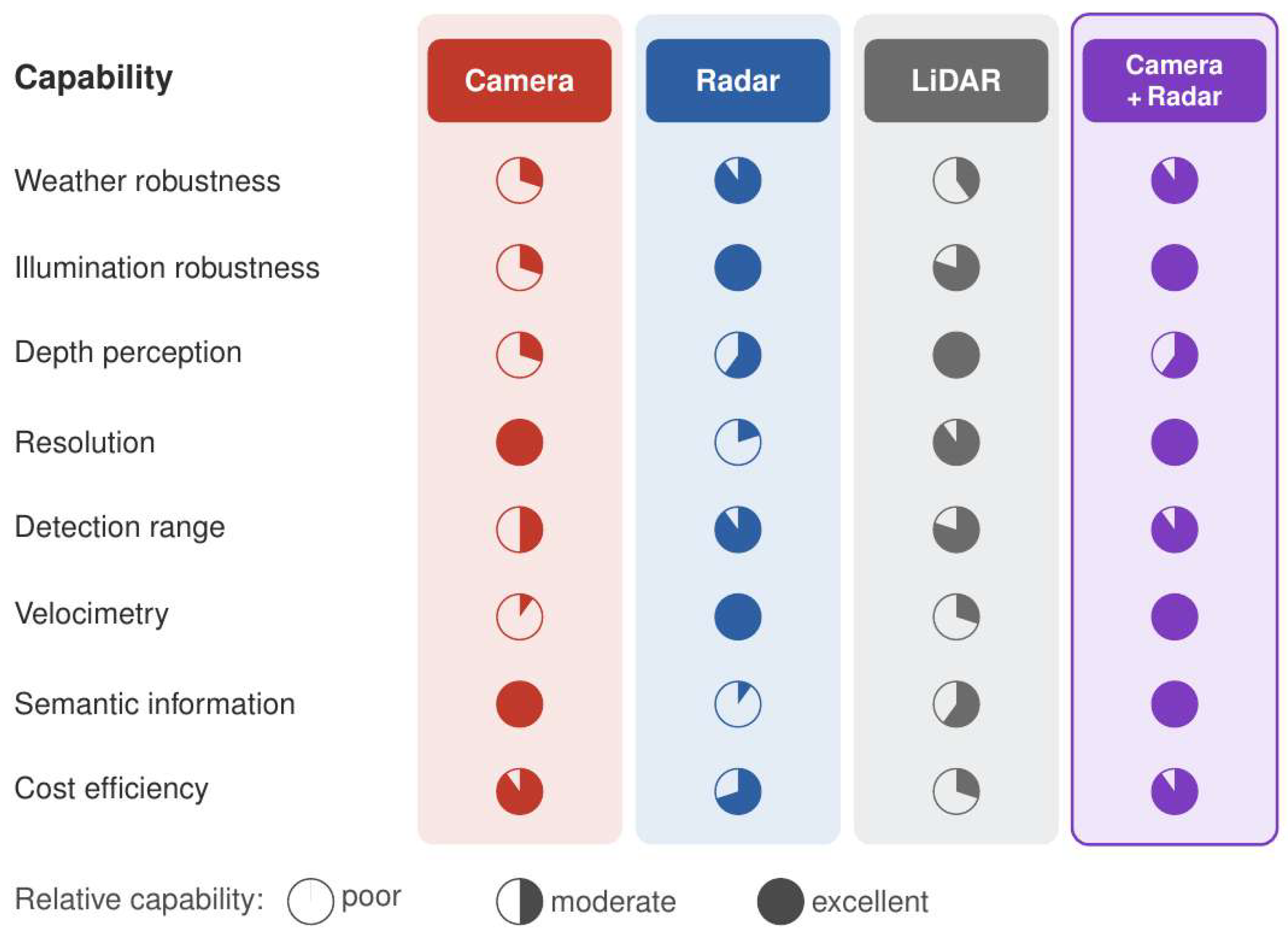
Over the past decade, various sensor fusion strategies have been developed to combine the complementary strengths of these modalities and develop reliable perception capabilities [16]. Different types of sensors offer complementary strengths, though each also has certain limitations, as shown in Figure 1. Through sensor fusion, it becomes possible to leverage these complementary characteristics to compensate for individual weaknesses, improving overall system performance under varying environmental conditions, including poor weather and low light [17]. There is increasing interest in utilizing multiple sensors for roadside applications to improve the perception capabilities of modern transportation networks [18,19,20].

While the fusion of camera and LiDAR data has driven notable progress in object detection [23,24,25,26], semantic segmentation [27,28], and multi-object tracking [29,30], both sensor types remain vulnerable to adverse environmental conditions such as fog, rain, and snow, which can degrade performance [31]. Moreover, the high cost and complexity of LiDAR systems continue to limit their scalability for large-scale deployment [32]. Many studies employ mmW radars in combination with cameras for sensor fusion, as they provide strong resilience against adverse weather and poor lighting conditions [13,14], while cameras provide rich semantic and visual detail. Fusing these complementary sources of information enables more robust and reliable perception across a broad range of real-world scenarios [33,34,35].

A distinct coordinate system and asynchronous frames are the major challenges in effective multi-sensor fusion [36]. Accurate fusion requires all sensors’ data to be in a common coordinate system; hence, calibration is required. Calibration must be performed initially and also periodically, as changes in environmental conditions or mechanical adjustments during maintenance can alter sensor alignment over time [11,37]. Therefore, calibration remains an essential and active area of research in the field of intelligent transportation. Although some aspects of this topic are addressed in broader reviews of sensor fusion [38,39], relatively few surveys have focused on extrinsic calibration between particular sensor pairs, such as LiDAR-camera [37,40] or multi-camera systems [41,42]. Given the increasing research focus on combining radar and camera sensors in roadside environments [16], there is a clear need for a focused and systematic review of calibration techniques for such systems. Unlike the dense 3D information provided by LiDAR, mmW radar is characterized by sparse and noisy point cloud returns, especially concerning elevation data, alongside artifacts like multipath and complex Radar Cross Section (RCS) effects. Crucially, most existing research targets vehicle-mounted platforms. This review distinguishes itself by specifically addressing the complex requirements of fixed roadside ITS deployments, which involve high mounting heights (typically 6–10 m) and severe perspective distortion, necessitating robust, scalable, online, and targetless calibration methods.

This review sets out to evaluate and synthesize the extrinsic calibration methods available for radar-camera systems on fixed roadside infrastructure. It pursues three aims. The first is to set out the operational and geometric conditions that separate roadside deployment from vehicle-mounted platforms, particularly the high mounting elevation and the perspective distortion it produces. The second is to compare classical two-stage pipelines, which keep correspondence registration and parameter estimation as separate steps, against end-to-end learning architectures, weighing them on accuracy, scalability, and computational cost. Finally, the review intends to assess the current landscape of evaluation metrics and underscore the necessity for standardized benchmarks to ensure robust, continuous calibration in dynamic urban environments. The main contributions of this comprehensive survey are as follows:

• Novel Focus on Roadside ITS: Provides one of the first dedicated reviews of radar-camera extrinsic calibration, emphasizing the unique challenges, such as high mounting heights, severe perspective distortion, and the need for online operation, that distinguish fixed roadside ITS deployments from vehicle-mounted systems.
• In-Depth Technical Comparison: Offers a critical and quantitative analysis of state-of-the-art methodologies, specifically detailing how systems overcome radar sparsity and noise through specialized techniques, including the comparative evaluation of nonlinear optimization solvers and the accuracy of track-to-track association methods.
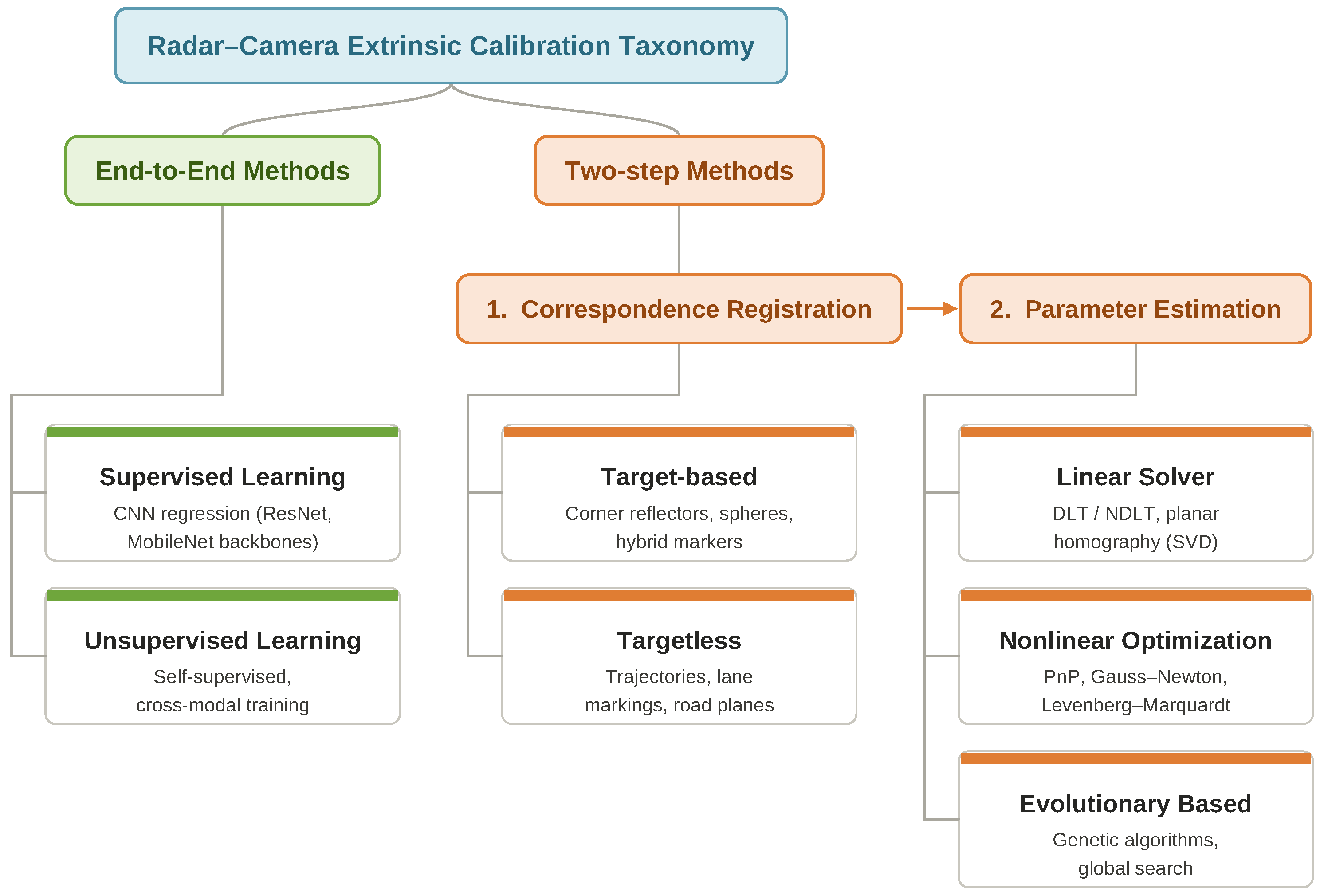
• Unified Taxonomy and Future Benchmarks: Introduces a clear, integrated taxonomy (two-step/end-to-end, target-based/targetless) and synthesizes practical deployment challenges, outlining explicit future directions for achieving full 6-DoF, continuous recalibration and establishing standardized benchmarks.

The remainder of this paper is structured as follows. Section 2 provides the detailed review methodology, providing a detailed account of the systematic review process conducted in accordance with the PRISMA 2020 guideline (Supplementary Materials). Section 3 introduces the background and problem definition of radar-camera calibration. Section 4 reviews data association techniques for two-step calibration, including both target-based and targetless methods; Section 5 then explains parameter estimation methods for two-step calibration. Section 6 discusses recent developments in end-to-end calibration approaches. Section 7 summarizes widely used evaluation metrics. In Section 8, the critical operational assumptions and environmental constraints of these methods are analyzed. Section 9 identifies open research challenges and provides a forward-looking roadmap for the field, and finally, Section 10 concludes the paper.

2. Review Method

To provide a comprehensive analysis of the literature on radar-camera extrinsic calibration techniques for roadside applications, a systematic literature search was conducted. The methodology is grounded in established systematic review frameworks, specifically adhering to the PRISMA 2020 guidelines [43] alongside the protocols outlined by Okoli et al. [44]. IEEE Xplore and Scopus were selected as the primary databases due to their extensive coverage of intelligent transportation systems and sensor fusion methodologies. To capture the most recent advancements, particularly regarding roadside implementations, supplementary searches were conducted using Google Scholar. All databases were last searched on 8 June 2026.

2.1. Refined Search Queries and Screening

The search strategy targeted literature published between 2015 and 2026, capturing the evolution from classical target-based methods to modern targetless, end-to-end, and learning-based approaches. The search queries combined keywords related to the sensors with calibration and application terms. The specific queries are listed in

Table 1. List of search queries utilized in the current survey analysis.

Domain	Query
IEEE Xplore	(“All Metadata”:“Radar” OR “All Metadata”:“mmW Radar” OR “All Metadata”:“millimeter-wave” OR “All Metadata”:“mmWave”) AND (“All Metadata”:“Camera” OR “All Metadata”:“Vision”) AND (“All Metadata”:“Calibration” OR “All Metadata”:“Alignment” OR “All Metadata”:“Spatial synchronization” OR “All Metadata”:“Auto-calibration” OR “All Metadata”:“Extrinsic”) AND (“All Metadata”:“On-road” OR “All Metadata”:“Roadside” OR “All Metadata”:“Infrastructure” OR “All Metadata”:“Intelligent Transportation” OR “ITS” OR “Smart intersection”)
Scopus	TITLE-ABS-KEY (“Radar” OR “mmW Radar” OR “millimeter-wave” OR “mmWave”) AND TITLE-ABS-KEY (“Camera” OR “Vision”) AND TITLE-ABS-KEY (“Calibration” OR “Alignment” OR “Spatial synchronization” OR “Auto-calibration” OR “Extrinsic”) AND TITLE-ABS-KEY (“On-road” OR “Roadside” OR “Infrastructure” OR “Intelligent Transportation” OR “ITS” OR “Smart intersection”) AND (PUBYEAR > 2014 AND PUBYEAR < 2027)
Google Scholar	(“Radar” OR “mmW Radar” OR “millimeter-wave” OR “mmWave”) AND (“Camera” OR “Vision”) AND (“Calibration” OR “Alignment” OR “Spatial synchronization” OR “Auto-calibration” OR “Extrinsic”) AND (“On-road” OR “Roadside” OR “Infrastructure” OR “Intelligent Transportation” OR “ITS” OR “Smart intersection”)

.

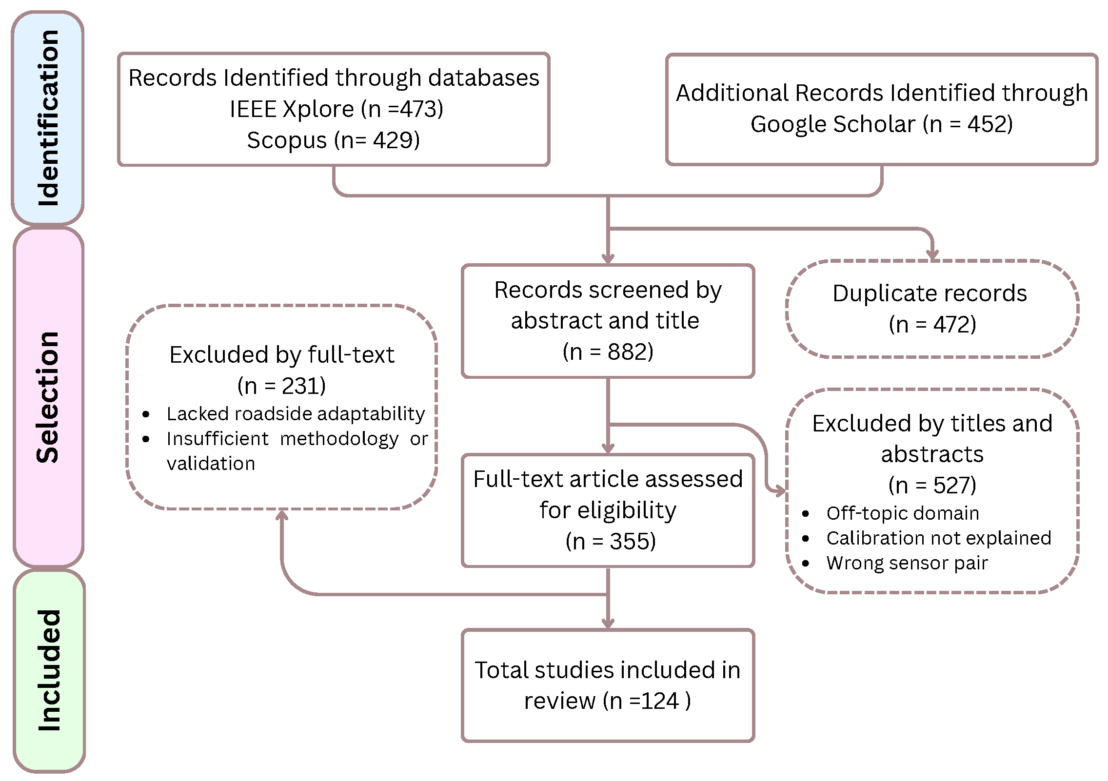
The initial search returned 473 records from IEEE Xplore, 429 from Scopus, and 452 from Google Scholar, for 1354 in total. IEEE Xplore and Scopus were queried directly through their advanced search interfaces. Google Scholar was used only as a supplementary source. It provides no option to export the full result set and ranks records by relevance rather than returning a complete, reproducible list. Because of this, its records were screened in descending relevance order and collection was stopped once results were no longer on-topic, which is readily apparent from the title alone. This kept Scholar’s role limited to surfacing recent or cross-disciplinary work that IEEE Xplore and Scopus might have missed. In the next step, duplicate records were removed by hand, matching on title, authors, and DOI; this discarded 472 records and left 882 unique studies for screening. Figure 2 shows the full screening flow as a PRISMA flow diagram.

The first author screened the 882 titles and abstracts against the inclusion and exclusion criteria, consulting the second author whenever a record’s relevance was unclear. This stage excluded 527 records and carried 355 forward to full-text assessment. At the full-text stage, 231 records were excluded. The two reasons were insufficient methodological or validation detail for the calibration procedure to be analyzed, and the absence of applicability to static or roadside deployment, for example, methods that depend on vehicle ego-motion during calibration.

Vehicle-mounted studies were included when their calibration procedure assumes a stationary sensor configuration during calibration, rather than relying on vehicle ego-motion. Although such setups lack the high mounting elevation of roadside infrastructure, their static calibration formulation makes them, in principle, applicable to roadside deployment, and they constitute the primary source of advanced correspondence and estimation techniques. Studies whose primary contribution is sensor fusion were also included when their extrinsic calibration methodology is reported in sufficient detail.

2.2. Inclusion Criteria

• Articles explicitly focusing on the extrinsic auto-calibration of mmW radar and monocular camera setups.
• Studies addressing calibration methodologies applicable to intelligent transportation systems, with a strong emphasis on roadside infrastructure and autonomous driving environments.
• Research proposing target-based, targetless, or learning-based correspondence registration and parameter estimation techniques.
• Peer-reviewed journal articles and high-impact conference proceedings.
• Studies developed for vehicle- or robot-mounted platforms were included only when their calibration procedure assumes a stationary sensor configuration, with no dependence on vehicle ego-motion, making the method transferable in principle to fixed roadside deployment.

2.3. Exclusion Criteria

• Studies focusing exclusively on the intrinsic calibration of sensors without addressing cross-sensor extrinsic alignment.
• Research dedicated to different sensor pairs (e.g., exclusively LiDAR-camera fusion) where radar is not included.
• Articles primarily focused on vehicle dynamics, uncertainty modelling, or general tracking algorithms that do not directly contribute to the sensor calibration process.
• Non-English publications, patents, and magazines.
• Studies proposing a calibration method but providing insufficient methodological or validation detail for it to be analyzed.
• Studies whose calibration relies on vehicle ego-motion or dynamic driving, with no applicability to static or roadside deployment.

Several studies were excluded during full-text screening because their primary focus was downstream applications rather than the calibration process itself. For instance, Zhang and Cao [45] introduced a joint radar and camera system, but primarily emphasized tracking reliability using a fusion-extended Kalman filter. Because they relied on standard homography-based sensor alignment rather than proposing novel extrinsic calibration methodologies, the study is not included in this review.

2.4. Data Extraction Process

Data extraction was performed manually by the first author using a standardized matrix, with the second author consulted on ambiguous methodological cases. The extracted fields included the correspondence registration method, the per-sensor detection methodology, the parameter estimation algorithm, the reported evaluation metrics, and the validation datasets, all taken directly from the published texts. The primary outcomes were quantitative accuracy metrics, namely geometric alignment errors (e.g., Average Rotation Error, Average Euclidean Distance) and projection error (e.g., Mean Reprojection Error); secondary outcomes were computational efficiency and the validation environment. Where a study reported multiple datasets or variants, priority was given to results on realistic outdoor or infrastructure data over simulated or indoor settings.

This review follows the PRISMA 2020 reporting structure, though some elements of clinical-grade methodology were not applied: screening relied on the first author with second-author consensus rather than independent dual screening, and the protocol was not pre-registered in PROSPERO. Clinical appraisal instruments such as ROBINS-I were not applicable, as they target clinical rather than engineering studies. Instead, the reviewed studies were appraised using a domain-specific framework of four criteria, summarized in

Table 2. Quality-assessment criteria applied to the reviewed studies.

Criterion	Question Used to Appraise the Study	Quality Indicator
Validation Rigor	Is calibration accuracy reported through quantitative error metrics, or only through qualitative or visual alignment?	Quantitative geometric or reprojection error indicates higher rigor than visual-only validation.
Validation Realism	Was the method evaluated on real-world field or roadside data, or only in simulation or controlled indoor settings?	Real-world outdoor or infrastructure data indicates higher external validity.
Ground-Truth Basis	Is accuracy measured against an independent ground-truth reference, or  only self-referentially?	Independent ground truth indicates a more reliable accuracy claim.
Methodological Transparency	Are the calibration procedure, parameters, and evaluation setup described in sufficient detail to be analyzed and reproduced?	Sufficient procedural detail indicates higher reliability.

: validation rigour, validation realism, ground-truth basis, and methodological transparency. These criteria were applied during full-text screening: studies were retained only when their calibration procedure and evaluation were reported in enough detail to be assessed against them, and the methodological-transparency criterion is enforced directly by the exclusion criteria, which removed studies lacking sufficient methodological or validation detail. Rather than assigning numerical quality scores, which the heterogeneity of reporting across these studies would not support reliably, the criteria are used qualitatively to frame the comparative discussion of accuracy, validation realism, and deployment constraints in the synthesis sections.

3. Background and Problem Formulation of Radar-Camera Calibration

Before detailing the specific calibration methodologies, it is necessary to define the mathematical notations and coordinate systems used throughout this paper.

Table 3. Summary of key mathematical notations.

Symbol	Definition
${\mathcal{F}}_r,{\mathcal{F}}_c$	Radar and camera coordinate systems.
${\mathbf{P}}_r,{\widehat{\mathbf{P}}}_r$	Observed and projected 3D point coordinates in the radar coordinate system.
${\mathbf{P}}_c,{\widehat{\mathbf{P}}}_c$	Observed and projected 3D point coordinates in the camera coordinate system.
$\mathbf{K}$	Camera intrinsic matrix.
$f_x,f_y$	Focal lengths along the image axes.
$f_s$	Skewness of image plane axes.
$(u_0,v_0)$	Principal point coordinates on the pixel coordinate system.
$\mathbf{q},\widehat{\mathbf{q}}$	Observed and projected points in the homogeneous pixel coordinate system.
$z_c$	Depth along the camera’s optical axis.
$\mathbf{T}$	Rigid transformation matrix mapping the coordinate frames.
${\mathbf{R}}_{cr},{\mathbf{t}}_{cr}$	Rotation matrix and translation vector mapping ${\mathcal{F}}_r$ to ${\mathcal{F}}_c$.
$\alpha ,\beta ,\gamma$	Euler angles representing roll, pitch, and yaw.
$t_x,t_y,t_z$	Translational displacements along the Cartesian axes.
$\pi (·)$	Projection function defined by sensor intrinsic parameters.
$\mathcal{L}(·,·)$	Predefined loss or error function for optimization.

summarizes the primary variables and coordinate frames utilized in the subsequent formulations.

3.1. Intrinsic Calibration

Intrinsic calibration characterizes the internal parameters of each sensor independently. It is an essential step to convert raw received signals into measurements that can be interpreted and processed consistently. For mmW radar sensors, intrinsic calibration procedures are less standardized compared to optical systems. Radar detections are generally reported in Spherical or Cartesian coordinates relative to the radar’s local frame, often including Doppler velocity measurements [46]. Intrinsic radar calibration aims to compensate for systematic biases such as antenna misalignment, phase distortions, and timing offsets. Although many modern radars are factory-calibrated, further intrinsic calibration may still be required for high-precision or safety-critical applications [47].

For cameras, intrinsic calibration is well established and typically involves estimating the intrinsic matrix $\mathbf{K}$, which models the pinhole projection [48] from 3D coordinates in the camera frame to 2D-pixel coordinates, as shown in (1):

$$\mathbf{K}=\left[\begin{array}{ccc}{f}_x& f_s& u_0\\ 0& f_y& v_0\\ 0& 0& 1\end{array}\right]$$

(1)

where $f_x$ and $f_y$ represent the focal lengths along the image axes, $f_s$ is the skewness of image plane axes [49], and $(u_0,v_0)$ is the principal point. In addition, lens distortion parameters are often estimated to correct geometric distortions introduced by the optics. Camera intrinsic calibration is commonly performed using planar checkerboard patterns after setting the focal length [50]. Once the camera intrinsic parameters are calibrated, they allow 3D points expressed in the camera coordinate system to be projected onto the 2D image plane. Consider a point ${\mathbf{P}}_c={[x_c,y_c,z_c]}^T$ in the camera coordinate frame. Its corresponding pixel coordinate $\mathbf{q}={[u,v,1]}^T$ in homogeneous image coordinates is obtained by using (2) [51].

$$z_c\mathbf{q}=\mathbf{K}{\mathbf{P}}_c$$

(2)

where $z_c$ is the depth along the camera’s optical axis. In this way, the intrinsic matrix $\mathbf{K}$ converts a 3D position in metric space to a 2D pixel location, allowing the data to be directly related to the image. If lens distortion is present, a distortion model can be applied after this projection to correct for radial and tangential effects. The combination of the intrinsic matrix and distortion parameters ensures that measurements from the camera can be consistently interpreted in pixel space.

3.2. Extrinsic Calibration

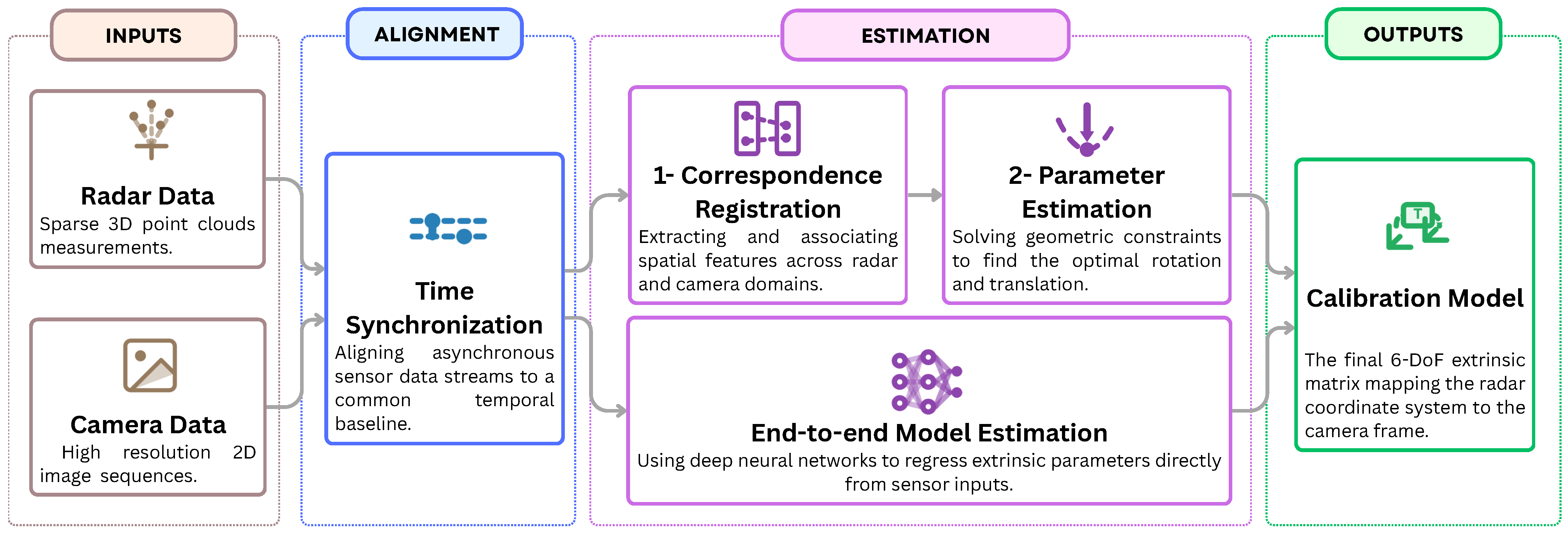
Extrinsic calibration determines the rigid transformation between different coordinate systems to align their data into a common frame. Each sensor operates in its own local coordinate system, and without an accurate spatial transformation between them, it is impossible to meaningfully relate observations across modalities. The fundamental architecture of this spatial alignment process is illustrated in Figure 3, which maps the flow from raw data acquisition and temporal synchronization to the final estimation of the transformation matrix. When two sensors are involved, extrinsic calibration defines a direct transformation between their local coordinate systems. However, the calibration is often formulated relative to a common global coordinate frame in systems involving more than two sensors, such as a multi-camera or radar-LiDAR camera setup. In such cases, each sensor’s pose is expressed as a rigid transformation with respect to this global frame, ensuring all sensor data can be mapped into a unified space.

The geometric relationship between radar and camera sensors is captured by a rigid transformation between their coordinate frames. Let ${\mathcal{F}}_r$ and ${\mathcal{F}}_c$ denote the radar and camera coordinate frames, respectively. A point ${\mathbf{P}}_r\in {\mathbb{R}}^3$, expressed in the radar frame ${\mathcal{F}}_r$, can be transformed into the camera frame ${\mathcal{F}}_c$ through a rotation and translation as described in (3):

$${\widehat{\mathbf{P}}}_c={\mathbf{R}}_{cr}{\mathbf{P}}_r+{\mathbf{t}}_{cr}$$

(3)

where ${\mathbf{R}}_{cr}\in {\mathbb{R}}^{3\times 3}$ is the rotation matrix that aligns the axes of the radar frame with the camera frame, and ${\mathbf{t}}_{cr}\in {\mathbb{R}}^3$ is the translation vector between the two sensor origins. This formulation assumes that both sensors share a common unit system (e.g., meters) and that time synchronization is sufficiently accurate to neglect motion during the transformation.

The point ${\widehat{\mathbf{P}}}_c={[x_c,y_c,z_c]}^T$, now expressed in ${\mathcal{F}}_c$, can be projected onto the 2D image plane using the camera’s intrinsic matrix $\mathbf{K}\in {\mathbb{R}}^{3\times 3}$. The resulting pixel coordinates $\widehat{\mathbf{q}}={[u,v,1]}^T$ in homogeneous form can be found by using the equation described in (4) [52].

$$z_c\widehat{\mathbf{q}}=\mathbf{K}{\widehat{\mathbf{P}}}_c=\mathbf{K}\left({\mathbf{R}}_{cr}{\mathbf{P}}_r+{\mathbf{t}}_{cr}\right)$$

(4)

This two-stage mapping, which is first from the radar frame to the camera frame, and then from the camera frame to the image coordinates, forms the backbone of radar-to-image alignment. It allows radar detections to be interpreted within the visual domain and serves as the mathematical foundation for defining the extrinsic calibration problem.

The goal of extrinsic calibration is to estimate the unknown transformation parameters such that the transformed data from one sensor best aligns with corresponding data in another sensor’s frame. This is typically cast as an optimization problem over a set of cross-sensor correspondences. Let $\left\{{\mathbf{P}}_i^k\right\}$ be points from sensor i, and $\left\{{\mathbf{q}}_j^k\right\}$ be their corresponding observations in sensor j’s domain (e.g., pixel coordinates in the camera image). The optimal transformation ${\mathbf{T}}_{ij}=[\mathbf{R},\mathbf{t}]$ minimizes the discrepancy between projected and observed data. A general formulation is:

$$\underset{\mathbf{R},\mathbf{t}}{\min }{\displaystyle \sum _{k=1}^N}\mathcal{L}\left({\mathbf{q}}_j^k,\pi \left(\mathbf{R}{\mathbf{P}}_i^k+\mathbf{t}\right)\right),$$

(5)

where $\pi (·)$ is the projection function defined by the intrinsic parameters of sensor j, and $\mathcal{L}(·,·)$ is a predefined loss function (e.g., Euclidean distance in image space). This flexible formulation allows for various types of correspondences, such as point-wise, edge-based, object-level, or learned features, to be incorporated depending on the sensors and methods used.

It is also important to note that many high-level sensor fusion frameworks operate under the assumption that extrinsic parameters are pre-calculated and static, or in order to reduce the complexity of full 6-DoF estimation, some approaches simplify the problem by leveraging specific structural constraints. Ref. [53] proposed a method where a single probe vehicle drives straight along a lane; assuming the sensors are co-located and levelled, they fit linear trajectories to the vehicle’s path in both sensor frames to calculate the azimuth (yaw) offset directly. In addition, methods presented in [54,55] bypass the calibration process entirely by relying on pre-calibrated datasets. However, Nabati and Qi explicitly highlighted that this reliance is non-trivial; unlike LiDAR, radar point clouds are sparse, and lack elevation data, and radar returns often correspond to object edges rather than geometric centers. These characteristics introduce spatial mismatch errors that ’pre-known’ calibration parameters cannot always resolve, necessitating robust, dedicated calibration methodologies [55], such as those reviewed in the following sections.

As noted in the calibration formulations, extrinsic calibration methods are traditionally structured into two sequential stages. The first involves identifying corresponding features, landmarks, or object trajectories within the overlapping field of view of the sensors. This data association step is essential for building reliable links across sensing modalities, such as radar and camera, which often differ significantly in resolution and perception characteristics. Once a sufficient number of correspondences have been established, the second stage solves an optimization problem to estimate the rigid transformation, typically expressed as a rotation and translation, that aligns the coordinate frames of the sensors.

Although this staged approach is still widely used, more recent work has begun to merge these steps into unified frameworks. Recent learning-based methods aim to combine correspondence identification and transformation estimation within a unified, end-to-end framework. These integrated approaches can simplify the process and make it more robust to noise and scene variability, particularly in dynamic environments where traditional assumptions may not hold, by minimizing dependence on handcrafted features or physical targets. An overview of the working principles of extrinsic calibration methods is presented in Figure 4. The assumptions and operational constraints for each category are detailed in the following sections.

4. Correspondence Registration

In traditional extrinsic calibration, there is a need to have a set of corresponding points from the objects observed by each sensor within their overlapping field of view, which is a time-consuming procedure [16]. This procedure, which is known as correspondence registration, can provide data for solving the transformation optimization problem described in (5). The associated points can be established using distinct objects and their characteristics as target-based approaches or by relying on scene features as targetless methods [56]. These two categories are discussed in detail in the following sections, emphasizing the algorithmic techniques and assumptions that define each approach.

4.1. Target-Based Association Techniques

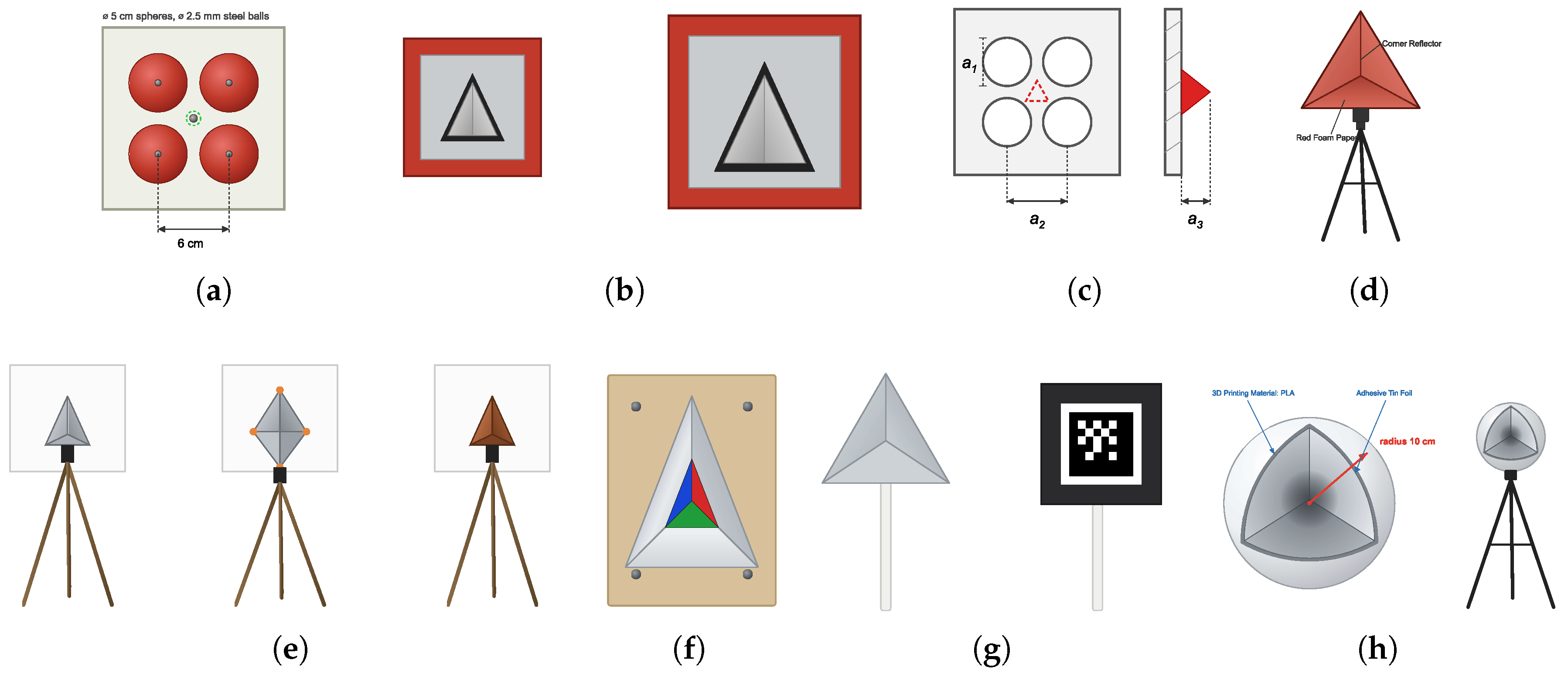
For calibration between radar and camera sensors, the target design must satisfy the sensing principles of both modalities. Radar units respond best to materials and shapes that provide a strong and stable RCS. Metallic trihedral corner reflectors or flat panels with highly reflective coatings are often used because they can return signals reliably from different incident angles [57,58,59]. Their drawback, however, is that in the visual domain they usually appear as blurred or indistinct objects, and this problem becomes more noticeable in outdoor scenes where illumination changes constantly. Cameras, on the other hand, require structured patterns that are visually salient and geometrically well defined—checkerboards, circle grids, or fiducial markers printed on planar high-contrast surfaces are typical choices [60]. These patterns are easy to detect in images but contribute little to radar measurements. The tension between the two sensing requirements has motivated the design of hybrid targets that bring the advantages together. A common strategy is to integrate small metallic reflectors into printed markers or to place radar reflectors adjacent to visual patterns, so that both sensors can extract the same geometric reference, such as a corner, centroid, or marker center. Examples include checkerboards or planar fiducials with embedded trihedral [61,62,63,64], radar-detectable augmented reality tags [65], and modified reflectors such as red-foam trihedral [66]. These solutions attempt to balance the complementary demands of radar and camera sensing and provide a physical feature set that both modalities can register consistently [67]. Figure 5 shows representative targets that have been proposed for radar–camera calibration.

Manual correspondence registration remains a reliable, high-precision baseline for applied sensor fusion. Kang and Kum employed a manual correspondence strategy where corner reflectors were placed at 19 distinct locations, and radar measurements were manually matched to pixel coordinates to solve for the homography matrix [72]. Alternatively, authors in [73] utilized a mechanical alignment approach, designing a custom 3D-printed mounting frame to empirically fix the relative geometry between the radar and camera. For larger-scale setups, using a target vehicle equipped with RTK-GNSS is also common; by driving it through the perception zone, global coordinates can be obtained to align radar and camera tracks [74].

Radar targets are usually recognized because of the strong reflections they produce compared with the surrounding environment. The geometry of the reflector plays the central role: trihedral and octahedral corner reflectors are used most often since their angled surfaces direct the incoming wave back toward the radar, giving a bright and consistent return [75]. The choice of material further enhances this effect; metals such as copper or aluminum are common because they maintain a predictable RCS even when the viewing angle changes [69]. In practice, detection starts with simple thresholding: points with unusually high intensity or RCS values are marked as likely candidates, and frame averaging is often applied to reduce random fluctuations [62]. Once these points are isolated, the reflector position can be estimated by calculating its centroid. Because radar data is typically sparse and noisy, this step is rarely sufficient on its own. Clustering methods such as Density-Based Spatial Clustering of Applications with Noise (DBSCAN) [76] or neighborhood growing techniques like Neighborhood-Graph-based Minimum Spanning (NGMS) [77] are then applied to separate genuine reflections from clutter and multi-path returns [68]. This combination of geometry, material choice, intensity filtering, and clustering forms the basis of most radar-based target detection strategies in calibration studies.

In camera-based calibration, the detection of targets generally begins with preprocessing steps that enhance their visibility against complex backgrounds. To increase reliability, image preprocessing steps, which are usually thresholding, morphological filtering, and contour selection, are typically employed to isolate the target from the background [66]. After this stage, different detection methods are chosen depending on the target design. Checkerboards or dot patterns are usually processed with corner or blob detectors [78]. While circle fitting with RANdom SAmple Consensus (RANSAC) can sometimes be used [62], it is not always stable when the circle is incomplete or partially occluded. In such cases, contour-based methods or the Circle Hough Transform tend to be more reliable for estimating the true center of the target [68]. Some works also rely on template matching, where a stored image of the target is matched against the input frame. This approach can handle cluttered scenes, but usually needs a refinement step, such as feature matching or optical flow, to correct the corner positions [70]. The effectiveness of visual detection depends heavily on lighting, background clutter, and image resolution, all of which must be considered when designing calibration setups. Fiducial markers like AprilTag boards [71] offer another solution. They are designed with encoded patterns that provide both identity and orientation, which helps when part of the board is occluded or when the illumination is uneven. More recently, deep learning approaches have been introduced, for example, retraining Mask Regions with Convolutional Neural Networks (R-CNN) on images of calibration targets, which also improves robustness under different viewpoints and lighting conditions [62].

Once calibration targets are detected in both radar and camera, the key step is to establish their correspondences. In the basic setups with a single reflector, this is usually done manually by aligning the extracted centers [79]. When several reflectors are placed, correspondences are often determined implicitly by exploiting the known spatial layout of the targets, such as fixed distances or predefined marker arrangements [68,71]. More recent studies have explored semi-automatic procedures, where radar detections are first clustered and then matched to camera features using centroid estimates, supported by temporal consistency when the target is observed across multiple frames [52]. Despite these developments, fully automated association remains uncommon in target-based calibration, mainly due to the sparsity and noise of radar measurements [80]. A summary of representative approaches for target-based correspondence registration, including calibration target specifications, target detection method for both sensors and the registration strategy, is provided in

Table 4. Summary of existing target-based correspondence registration methods.

Ref. (Year)	Calibration Target	Radar Target Detection Method	Camera Target Detection Method	Cross-Sensor Correspondence Method	App.
[62] (2023)	Multiple trihedral corner reflectors mounted on styrofoam boards	Expected RCS range and high intensity	Feature extraction using a Mask-RCNN model	Direct manual association	Roadside
[66] (2024)	Modified trihedral corner reflector with red foam surfaces	Centroid of high intensity cluster using DBSCAN	Color thresholding, centroid calculation	Direct manual association	Vehicle
[67] (2022)	Metal coated spherical-trihedral reflector	Intensity-based detection	Contour detection in thermal image	Direct manual association	Roadside
[69] (2024)	Trihedral and octahedral aluminum/copper corner reflectors	Intensity-based detection	Manual selection of pixels	Direct manual association	Vehicle
[68] (2024)	Four Styrofoam spheres with embedded metal balls + central ball reflector	RCS thresholding + clustering (GreedyNMS/Euclidean)	Circle detection on RGB-D with filtering and RANSAC	Direct manual association using known geometry	Roadside
[71] (2023)	Trihedral retroreflector combined with AprilTag fiducial on cardboard backing	Intensity-based detection	AprilTag detected by standard fiducial marker extraction	Direct manual association using known geometry	Vehicle
[81] (2021)	Styrofoam board with 4 holes and central trihedral reflector	Expected RCS range	Circle detection in 2D image	Direct manual association	Vehicle
[82] (2025)	Board with holes + AprilTags + radar Doppler simulator	Doppler simulator echo in range-Doppler cube	AprilTag corner detection (sub-pixel)	Known target geometry;probabilistic uncertainty-weighted optimization	Vehicle

.

4.2. Targetless Association Techniques

A key advantage of targetless correspondence registration is that it eliminates the need for dedicated calibration objects or controlled environments. This makes it possible to perform recalibration periodically without disrupting traffic flow [83,84], an aspect that is particularly valuable in long-term deployments where access to the sensor setup is constrained. Such methods allow the calibration parameters to be maintained over the full lifecycle of the sensors, thereby ensuring accuracy and reliability in intelligent transportation systems that require online or continuous recalibration [85]. The main difficulty, however, is the identification and alignment of features that are jointly observable in radar and camera data, such as track-to-track association [86]. In the absence of predefined targets, calibration must instead rely on naturally occurring cues such as vehicle trajectories [83,87], lane markings [88,89], or other stable scene structures [90]. Consequently, recent research on roadside sensor calibration is increasingly shifting toward targetless strategies, highlighting their potential as a practical and sustainable solution for maintaining multi-sensor precision. A summary of representative approaches for targetless correspondence registration is provided in

Table 5. Summary of existing targetless correspondence registration methods.

Ref. (Year)	Target Feature	Radar Target Detection Method	Camera Target Detection Method	Cross-Sensor Correspondence Method	App.
[91] (2025)	Vehicle trajectory events (lane change, turn, straight)	Extracts trajectory events from radar tracks	Extracts trajectory events from image tracks	Multi-stage event association (cross-ratio + frame-distance-domain matching)	Roadside
[90] (2021)	Lane features + vehicle trajectories	DBSCAN clustering + Kalman tracking	Lane line corner points + multi-object tracking	Virtual detection lines + Hungarian algorithm	Roadside
[92] (2024)	Vehicle trajectories under low/high traffic	Radar detection + trajectory tracking	Camera detection + trajectory tracking	Coarse MSED (low traffic), Hungarian algorithm (high traffic)	Roadside
[93] (2025)	Multiple dynamic object trajectories	Radar trajectory tracking + RCS-based weighting	Camera trajectory tracking	Graph-based spatial topology matching + RANSAC	Roadside
[94] (2021)	Moving object tracks (vehicles, pedestrians)	Radar/LiDAR tracking	Camera tracking	Track-to-track association using velocity and position norms	Vehicle
[95] (2023)	Common learned features (deep YOLO-based)	Radar Range-Doppler-Angle features	Camera object features via YOLO	Learned common feature discriminator + PnP-RANSAC matching	Roadside
[96] (2024)	Vehicle trajectories (first/second order traits: velocity, relative distances)	Radar trajectory tracking	Camera trajectory tracking	Graph-based multi-target matching	Roadside
[89] (2022)	Lane centrelines + vehicle trajectories	Radar vehicle trajectories fitted with cubic polynomials	HD map lane centrelines	Lane-wise trajectory association	Roadside
[97] (2025)	Moving object tracks (vehicles, pedestrians)	Radar tracks (DBSCAN + Kalman + Hungarian)	Camera tracks (YOLOv5 + SORT)	Track-to-track association via self-calibration error + Hungarian	Roadside
[98] (2025)	Common learned features + moving object tracks	RadarYOLO on Radar heatmaps (RAD data)	YOLOv4 object detection	Common-feature discriminator matching + block-based sampling	Roadside
[99] (2025)	Vehicle position, velocity, and shape (Gaussian-modeled)	2D radar targets extended to 3D via RCG ground mode	YOLOv11 instance segmentation	Matching-free Bhattacharyya-distance loss	Roadside

.

Many targetless calibration approaches rely on the motion of vehicles to establish correspondences between the radar and the camera. For the camera, moving objects are detected through state-of-the-art vision models, with the You Only Look Once (YOLO) family [100] currently regarded as one of the most effective for this task. Earlier networks, such as EfficientNet [100], SSD [101], and DetectoRS [102], are also widely applied. These models not only provide bounding boxes and object classes but also allow the relative position of vehicles to be estimated, and under favourable conditions, their range can extend well beyond typical roadside requirements [90]. Once detections are obtained, multi-object tracking methods commonly use trackers such as SORT [103,104] or its deep-learning variant, such as StrongSORT [105] or DeepSORT [106], to maintain trajectories over time. In the case of radar, the situation is more complex. Measurement noise [107]. The lack of consistent target identifiers [90] make it difficult to recover trajectories directly from raw outputs. To overcome this, clustering methods are applied to group detections into meaningful tracks. Both k-means and DBSCAN have been widely used [108,109], though k-means often struggles with the irregular, nonconvex paths that vehicles follow [87]. DBSCAN has therefore become a preferred choice, as it groups points based on local density rather than strict geometric assumptions [110,111]. Radar trajectories are then stabilized using tracking frameworks, most often Kalman filters or deep learning-based trackers, which integrate velocity and timestamp information to reduce ambiguities when multiple vehicles overlap in the same lane [112]. In order to extract more features, the trajectories can also be parametrized using B-Spline, or Gaussian Process (GP) trajectory representation [71,85,113].

Track-to-track association has emerged as a practical approach within targetless correspondence registration. In this framework, trajectories independently obtained from radar and camera sensors are matched to establish cross-modal correspondences. Unlike traditional point- or feature-based registration, this strategy exploits temporal consistency and motion patterns, making it particularly resilient in dynamic traffic scenes. By focusing on the temporal evolution of objects rather than instantaneous detections, these methods provide a more robust foundation for sensor fusion in complex environments.

Recent literature highlights several strategies for refining this matching process. For example, Ref. [91] adopts a two-step approach that employs cross-ratio distance to align different types of trajectory events, such as lane changes and turning maneuvers. Other frameworks incorporate secondary data to reinforce stability, such as using radar cross-section values and spatial topology graphs [93]. To handle varying traffic volumes, researchers have transitioned from simple Euclidean distance minimization in low-density scenarios to more complex global assignment strategies, such as the Hungarian algorithm [114], to maintain consistency in crowded conditions [92,97].

A recent roadside method reformulates correspondence as the alignment of probability distributions rather than discrete points [99]. Radar and camera targets are each represented as Gaussian models capturing position, velocity, and shape, and a calibration loss based on the Bhattacharyya distance between the projected radar and segmented camera models is minimized directly, avoiding an explicit target-matching step. To compensate for radar’s missing elevation, the method introduces a radar–camera–ground model that constrains target height using the road plane, recovering the full set of extrinsic parameters from only the 2D positions that traffic radar typically reports.

Despite the growing sophistication of these matching algorithms, a significant gap remains in how they are validated. As summarized in

Table 6. Track-to-track association performance reported in selected radar-camera calibration literature.

Ref. (Year)	Association Method	Accuracy	App.
[94] (2021)	Calibration-agnostic track-to-track association (velocity-position norm difference)	94%	Vehicle
[96] (2024)	Graph-matching with Gaussian Process trajectory interpolation	90%	Roadside
[97] (2025)	Cost-matrix based track association	96.43%	Roadside
[85] (2024)	Motion + interaction feature–based trajectory matching	97%	Roadside

, only a few studies explicitly report the quantitative accuracy of the correspondence step itself. This lack of rigorous reporting suggests that much of the existing literature assumes the quality of the matching process rather than treating it as a variable that requires independent evaluation. Addressing this oversight is essential for ensuring the reliability of downstream calibration and tracking tasks.

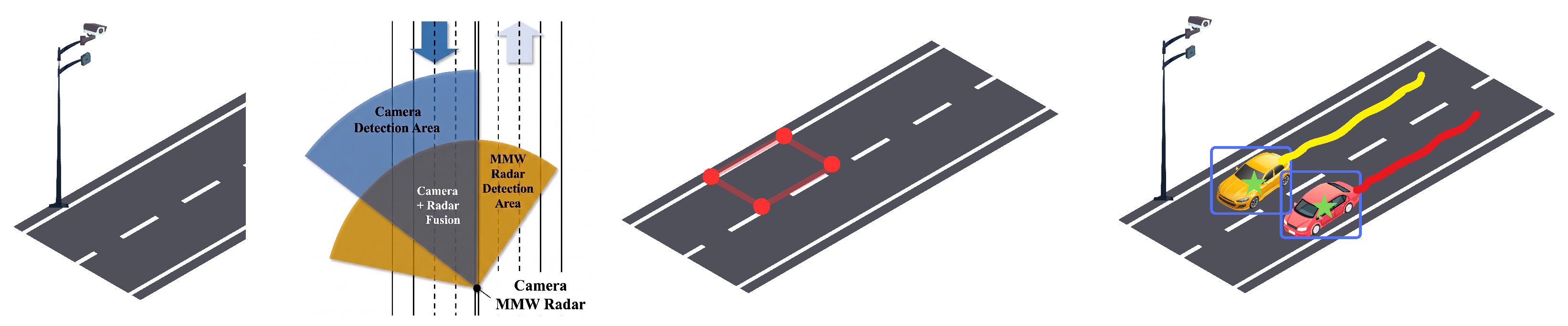
Road geometry provides dependable cues for radar–camera correspondence, especially in roadside applications where lane structures and road surfaces remain stable over time. Lane markings visible to the camera are used to provide initial alignment, while virtual detection lines drawn along the roadway generate events whenever vehicles cross them; these events can then be paired with radar observations, and the associations are solved with a Hungarian assignment strategy [90] as demonstrated in Figure 6. Another study makes use of vehicle trajectories captured by the radar itself, clustering them by lane and fitting cubic polynomials to approximate the lane centerline, which are later matched with lane references from high-definition maps in WGS-84 coordinates [89]. A different perspective relies on the geometry of the road plane: by identifying vehicle bottom points in both modalities and applying a RANSAC-based [115] fitting procedure, the underlying surface can be reconstructed and used as the shared feature for calibration in FusionCalib [83]. These examples illustrate how geometric information, whether extracted from lane markings, centrelines, or the road plane, can anchor correspondence registration when object-level associations are noisy or sparse.

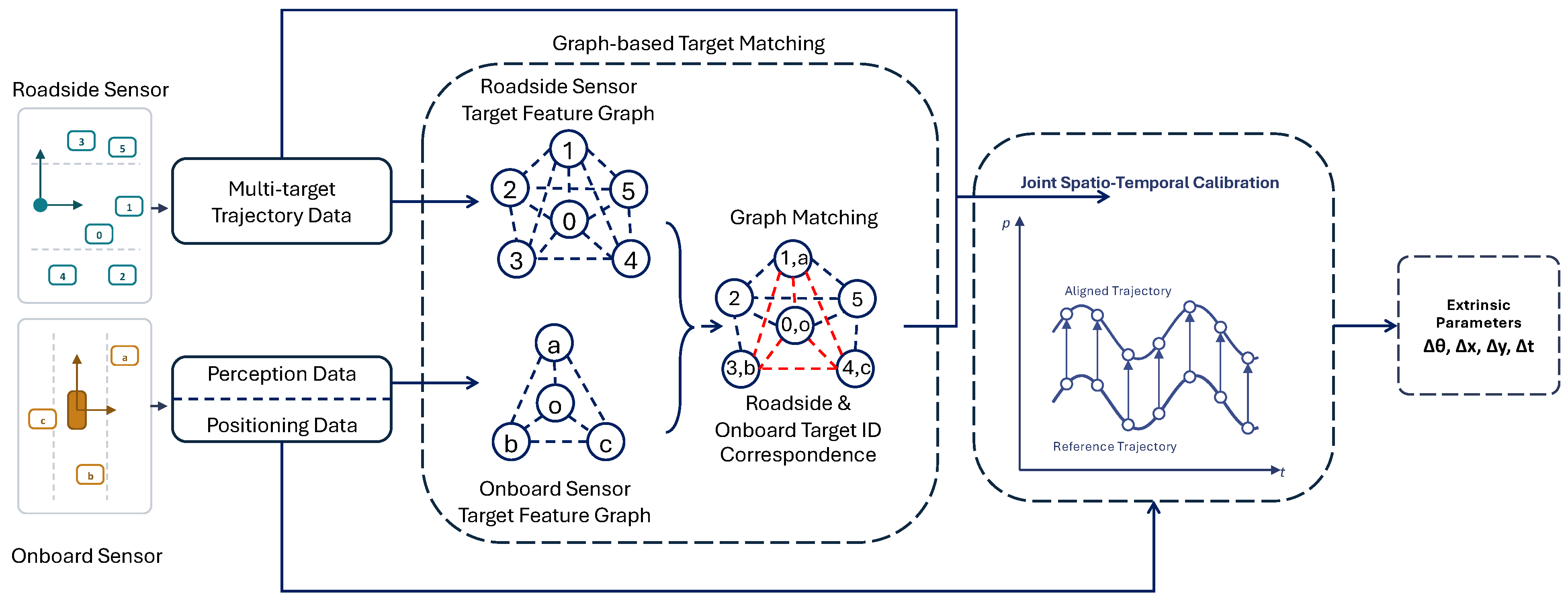
Beyond pairwise or feature-based techniques, graph-based methods have also emerged as a promising direction for correspondence registration. Graph-based methods approach correspondence registration by representing traffic scenes as networks, where each vehicle or moving object is treated as a node, and the edges describe how these objects relate to one another over space and time [94]. Instead of relying only on pairwise matches, this representation captures both individual motion and the structure of the scene. The study [93] applies this idea by forming directed graphs from radar and camera trajectories, in which edge weights reflect the relative positioning of trajectories, while radar cross-section values are used to emphasize more reliable detections. This weighting method reduces the influence of noisy tracks and enables stable calibration during long-term operation in dynamic environments. A more detailed version is proposed in [96], in which nodes still represent vehicles, but edges combine absolute motion features, such as velocity, with second-order descriptors like inter-vehicle distance and relative speed. The alignment of the two graphs is solved using the Graduated Non-Convexity and Concavity Procedure (GNCCP) [116], while Gaussian Process regression provides continuous interpolation of trajectories to handle asynchronous data. Their workflow, shown in Figure 7, illustrates how radar and camera trajectories are first encoded as graphs and then matched to designate consistent correspondences. By considering both motion and interaction patterns, this approach achieves reliable registration even in dense and complex traffic where simpler association rules often fail.

Another class of correspondence registration methods relies on exploiting shared features that are simultaneously observable by both radar and camera. Rather than associating geometric primitives such as lane markings or entire object trajectories, these approaches employ learned feature representations to establish cross-sensor matches in a more flexible manner. In [95], a YOLO-based network is trained to extract features from radar range–azimuth–Doppler data and camera images, followed by a discriminator that identifies whether radar and camera detections belong to the same object. By aligning the centers of matched detections, radar–camera correspondences are formed without the need for physical targets or handcrafted features. This feature-driven registration provides a flexible online solution, though its effectiveness depends on the quality of feature learning and may degrade in cluttered or crowded environments. This line of work was later extended into a radar–camera fusion framework for multi-object tracking [98], where the same common-feature discriminator drives online calibration between the radar range–azimuth plane and the camera image, adding block-based sampling for even correspondence distribution and a separate near/far homography fit to reduce projection error at range.

When evaluating correspondence registration as a whole, a distinct trade-off emerges between operational feasibility and spatial precision. Target-based methods achieve superior accuracy because they establish exact, point-level geometric anchors that both sensors can reliably detect. However, their primary failure mode is operational: they demand controlled environments, extensive human intervention, and highly disruptive road closures, making them unscalable for continuous infrastructure maintenance. Conversely, targetless methods resolve these operational bottlenecks by exploiting natural traffic flow, enabling continuous online recalibration. Yet, this operational freedom comes at the cost of peak accuracy. Because targetless approaches generally rely on object-level associations using bounding box centroids or fluctuating vehicle trajectories, they inherently lack the sub-pixel, point-level exactness of dedicated corner reflectors. Furthermore, targetless methods introduce their own environmental and traffic-dependent failure modes; trajectory-based matching frequently fails to converge in low-density traffic, while feature-based matching degrades sharply under poor illumination or adverse weather. The system designer is therefore forced to choose between the rigorous accuracy of an offline, point-level target and the practical, albeit noisier, object-level adaptability of targetless tracking.

5. Extrinsic Calibration Parameters Estimation

In the next phase, after matching radar and camera observations, the calibration parameters are estimated. In extrinsic calibration, these parameters generally consist of three translational and three rotational components, together forming the rigid-body transformation that maps a point from the radar coordinate frame ${\mathcal{F}}_r$ into the camera coordinate frame ${\mathcal{F}}_c$. A point $P_r={[X_r,Y_r,Z_r]}^T$ expressed in the radar frame is transformed into the camera frame $P_c={[X_c,Y_c,Z_c]}^T$ as in (6):

$$\left[\begin{array}{c}{X}_c\\ Y_c\\ Z_c\\ 1\end{array}\right]=\mathbf{T}\left[\begin{array}{c}{X}_r\\ Y_r\\ Z_r\\ 1\end{array}\right],$$

(6)

where the homogeneous transformation matrix $T\in {\mathbb{R}}^{4\times 4}$ is:

$$\mathbf{T}=\left[\begin{array}{cccc}{C}_{\alpha }{C}_{\beta }& C_{\alpha }{S}_{\beta }{S}_{\gamma }-S_{\alpha }{C}_{\gamma }& C_{\alpha }{S}_{\beta }{C}_{\gamma }+S_{\alpha }{S}_{\gamma }& t_x\\ S_{\alpha }{C}_{\beta }& S_{\alpha }{S}_{\beta }{S}_{\gamma }+C_{\alpha }{C}_{\gamma }& S_{\alpha }{S}_{\beta }{C}_{\gamma }-C_{\alpha }{S}_{\gamma }& t_y\\ -S_{\beta }& C_{\beta }{S}_{\gamma }& C_{\beta }{C}_{\gamma }& t_z\\ 0& 0& 0& 1\end{array}\right],$$

(7)

with $S_x=sinx$ and $C_x=cosx$.

In the transformation matrix defined in (7), the parameters $\alpha$, $\beta$, and $\gamma$ denote the Euler angles representing rotations about the x-, y-, and z-axes, respectively. These angles correspond to roll ($\alpha$), pitch ($\beta$), and yaw ($\gamma$), and together describe the relative orientation between the radar and camera coordinate frames. The terms $t_x$, $t_y$, and $t_z$ represent the translational displacements along the three Cartesian axes, forming the translation vector. The upper-left $3\times 3$ block of T thus encodes the rotation matrix $R_{cr}$, while the rightmost column encodes the translation vector $t_{cr}$, together defining the full 6-DoF rigid-body transformation between the two frames. Accordingly, the goal of the extrinsic parameter estimation stage is to predict the six extrinsic parameters, namely the three rotation angles and the three translation components, that minimize the calibration objective defined in (5), while K remains fixed.

If the rigid-body structure is not enforced and the combined mapping from radar coordinates directly to pixel coordinates is instead treated as a generic $3\times 4$ matrix, the relationship can be expressed as the linear system in (8). This formulation absorbs both the extrinsic transformation and the intrinsic projection into a single matrix without preserving orthogonality of the rotation component. This system of linear equations can be solved using the Direct Linear Transformation (DLT) method [72,117,118] or the modified Normalized Direct Linear Transformation (NDLT) [69], both based on Singular Value Decomposition (SVD). When the radar returns are further assumed to lie on a common ground plane ($Z=0$), the $3\times 4$ matrix reduces to a $3\times 3$ planar homography. The principal disadvantage of these linear methods is their limited accuracy and reliance on substantial pre-known information [51], since the solution does not enforce the rigid-body transformation constraint. Nevertheless, this formulation provides a useful coarse initialization, serving as a warm start for the subsequent nonlinear optimization problem [119].

$$\left[\begin{array}{c}{u}_i\\ v_i\\ 1\end{array}\right]=\left[\begin{array}{cccc}{p}_{11}& p_{12}& p_{13}& p_{14}\\ p_{21}& p_{22}& p_{23}& p_{24}\\ p_{31}& p_{32}& p_{33}& p_{34}\end{array}\right]\left[\begin{array}{c}{X}_i\\ Y_i\\ Z_i\\ 1\end{array}\right]$$

(8)

One of the most commonly used formulations in 2D–3D calibration is based on the Perspective-n-Point (PnP) problem, which is formulated as (5), as a nonlinear optimization problem. When the intrinsic parameters of the camera are known, PnP solvers can estimate the pose of the camera relative to a set of 3D points by minimizing the difference between observed image locations and the reprojected 3D points. Many works implement this through OpenCV’s solvePnP routine, often combined with RANSAC to handle outliers [95,120]. These methods are favoured for their speed and integration with existing computer vision pipelines. However, their accuracy greatly relies on the quality of the matches between the 2D and 3D data.

This nonlinear optimization calibration problem can be approached using a range of iterative and heuristic methods, including but not limited to Sequential Quadratic Programming for Perspective-n-Point (SQPnP) [121], Gauss–Newton (GN) [71,122] and Levenberg–Marquardt (LM) [119,123] using popular solvers like Ceres [124], as well as gradient-free strategies such as Genetic Algorithms [125].

Table 7. Comparison of parameter estimation methods used in radar-camera extrinsic calibration.

Method	Initialization Sensitivity	Strengths	Limitations
DLT/NDLT	None required	Closed-form via SVD; fast; useful as warm start	Low accuracy; does not enforce rigid-body constraints
PnP + RANSAC	Low	Robust to outliers; widely available in standard libraries	Depends on quality of 2D–3D correspondences
Gauss–Newton	High	Quadratic convergence near minimum; low per-iteration cost	Unstable with poor initialization or singular Jacobians
Levenberg–Marquardt	Moderate	Robust to poor initialization; default in Ceres and similar toolboxes	Higher per-iteration cost than GN; unconstrained only
SQP/SQPnP	Moderate	Handles nonlinear constraints (orthogonality, bounds)	Higher complexity; slower convergence
Genetic Algorithms	None (global search)	Gradient-free; explores non-convex spaces	High latency; impractical for online recalibration

provides a comparative summary of the principal parameter estimation methods, contrasting their initialization sensitivity, strengths, and limitations.

GN provides rapid, quadratic convergence near the minimum, but it suffers from instability if the initial guess is poor or if the Jacobian matrix becomes singular [126]. This makes GN risky for radar-camera calibration, where initialization (e.g., from PnP) might be coarse due to radar noise. In contrast, the LM algorithm, often the default choice in calibration toolboxes like Ceres, introduces a damping factor that interpolates between the Gauss-Newton method and gradient descent. This makes LM significantly more robust to poor initialization and rank-deficient Jacobians at a slightly higher computational cost per iteration [119].

Both GN and LM are typically designed for unconstrained least-squares problems. For setups requiring strict geometric constraints, such as enforcing specific mounting bounds or ensuring orthogonality in the rotation matrix without minimal parameterization, Sequential Quadratic Programming (SQP) is superior. SQP solves a sequence of quadratic sub-problems, allowing it to explicitly handle complex nonlinear constraints, though this comes with higher computational complexity compared to unconstrained solvers [127]. Therefore, LM is generally preferred for speed in online applications, while SQP is favoured when physical constraints must be rigorously enforced.

To enhance robustness and convergence, simplifying assumptions are often introduced, such as neglecting translational components, restricting orientation to a dominant axis, or leveraging prior knowledge of the scene [85,88,91,97]. Several studies go beyond the traditional PnP setup by formulating calibration as a nonlinear least squares problem with a combination of point-to-plane and point-to-backprojected-plane constraints to find the geometry between radar detections and the camera image [62]. In [81], the calibration problem is formulated through iterative alignment using point-to-line distances, which is suitable for radar data where reflectors appear as long structures. These formulations can provide more control over the calibration behaviour, particularly in scenarios with limited or noisy correspondences.

Alternative approaches employ constrained optimization methods to ensure the resulting solution adheres to specific structural requirements. For instance, in [63], three configurations of the optimization problem are introduced and solved using Sequential Least Squares Quadratic Programming (SLSQP), allowing the inclusion of constraints like rotation orthogonality and bounded translations. This enables precise control over the evolution of parameters during optimization, ensuring physically plausible solutions. This idea can be extended to not only include spatial transformation but also scales and temporal offset [90], making it suitable for asynchronous sensor setups. While these methods tend to be more computationally demanding, they offer greater flexibility in tailoring the calibration process to the specific characteristics of the system.

Road reconstruction can also serve as the primary geometric reference for extrinsic parameter estimation. A notable implementation, FusionCalib [83], detects vehicle bottoms in camera images through vanishing point geometry combined with Mask-RCNN segmentation. These detections are matched with radar trajectories using the Clue-Aware Trajectory Similarity (CATS) metric, which evaluates both spatial and temporal consistency to establish reliable cross-sensor associations. Once associated, the 2D pixel positions from the camera and 3D velocities from radar are fused through an Extended Kalman Filter, producing a set of 3D vehicle bottom positions that are assumed to lie on the road surface. A RANSAC-based fitting procedure then reconstructs the road plane from these sampled points. The normal of the fitted plane constrains pitch and roll, the traffic flow direction from vanishing points provides yaw, and translation is determined by aligning the sensor origin with the plane. In this way, defining constraints can enhance the accuracy of solving the nonlinear optimization problem.

When analytical solutions are difficult to apply and become highly non-convex, heuristic or evolutionary algorithms have been proposed. Genetic Algorithms (GA) are often used in this context, as they do not require gradient information and can explore a wider solution space. In [125], multi-objective versions like NSGA-II (Nondominated Sorting Genetic Algorithm II) [128] have been utilized to balance conflicting goals, which are defined as maximizing the number of associated points while minimizing their distance to bounding box centers. These methods are especially effective in complex environments where traditional gradient-based solvers may have difficulty converging.

Evaluating parameter estimation techniques highlights a direct trade-off between computational stability, geometric adaptability, and processing speed. Closed-form linear solvers like the DLT provide exceptionally fast computations. The drawback is their mathematical leniency; because they do not strictly enforce rigid-body constraints, they can easily output physically impossible transformation matrices. Gradient-based nonlinear optimizers (e.g., Levenberg-Marquardt and Gauss-Newton) solve this by enforcing strict geometric rules, but they introduce a different failure mode. If the initial guess is poor, these solvers become extremely sensitive to initialization and consistently get trapped in local minima. Global search methods, including GA, avoid this initialization problem entirely since they do not rely on gradients. The cost, however, is severe computational latency that makes them largely impractical for continuous online recalibration. To prevent false convergence in gradient solvers, researchers often reduce the estimated degrees of freedom by relying on prior knowledge of the sensor structure, commonly by fixing pitch and roll to only estimate yaw. This constraint-heavy approach certainly forces a safer mathematical convergence. Unfortunately, it severely restricts the framework’s adaptability across diverse roadside infrastructure setups where mounting angles are unpredictable.

6. End-to-End Radar-Camera Calibration Methods

While traditional radar-camera calibration relies on decoupled, multi-stage pipelines, typically involving separate algorithms for target detection, correspondence registration, and parameter estimation, recent literature demonstrates a transition toward integrated, end-to-end architectures. By embedding the calibration process within a unified neural network or differentiable solver, these methods directly regress or optimize the spatial transformation between sensors. This paradigm reduces the reliance on handcrafted feature extraction and explicit correspondence registration, thereby offering a higher degree of automation. Such autonomy is particularly advantageous for continuous online recalibration in dynamic environments, where deploying physical calibration targets is operationally unfeasible. To provide a structured analysis of these emerging data-driven techniques, the following subsections categorize current methodologies into two distinct paradigms based on their supervision signals and architectural constraints.

A representative example in this category is the work of Schöller et al. [88], who introduced a fully learning-based targetless method to estimate the rotational offset between radar and camera sensors. Their architecture comprises two convolutional neural networks: a coarse model that predicts an initial rotational correction and a fine model trained on the residual error of the first. The radar input is projected into the camera view using an initial transformation, and a boosting-inspired two-stage training regime is used to refine the misalignment. This network learns to implicitly associate radar detections with vehicle positions in the image, using only geometric alignment cues as supervision. To obtain sufficient training data, the authors first collected real-world radar–camera measurements from highway gantry bridges and established ground-truth calibration manually. They then synthetically augmented the dataset by applying random decalibrations to the ground-truth extrinsics, producing 34,000 samples across a wide range of rotational errors. The fine network was trained on residual errors after coarse correction, enabling it to specialize in subtle misalignments. Performance was validated on independent test sets, including one from a different sensor installation, showing the model’s ability to generalize to unseen environments. However, the approach is restricted to rotational calibration and does not estimate translations, which limits its applicability when full six-degree-of-freedom extrinsics are required.

Liu et al. [129] proposed an online intelligent radar–camera calibration framework based on deep neural networks. Training data are collected automatically during operation by exploiting ideal environments, where only a single object passes through the scene, so that the radar trajectory and the camera detection can be paired unambiguously. Once such data are identified, radar and camera measurements are synchronized with timestamps, stored, and filtered to ensure quality and balance. The dataset is then expanded and divided into training and test sets, with the neural network trained online and its accuracy evaluated on the test subset. This process enables the model to adapt to new environments without requiring manual recalibration. However, the approach depends on single-object conditions for reliable data collection and imposes high computational and storage demands due to repeated online training, which constrains its real-time applicability.

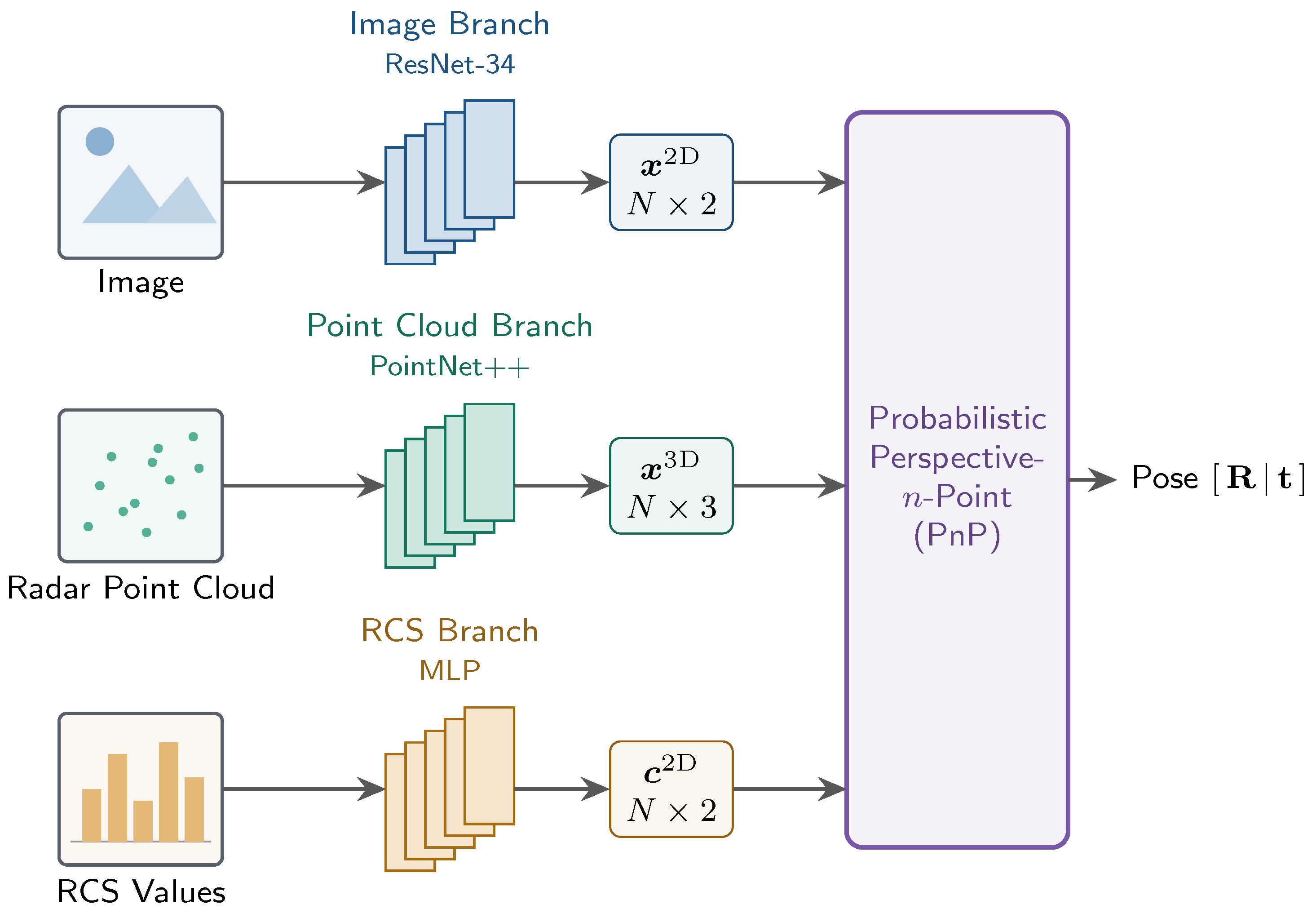
Zhang et al. [130] proposed a differentiable targetless radar–camera calibration method that leverages radar detection attributes to overcome the sparsity and uncertainty of mmW point clouds. As shown in Figure 8, their framework employs a three-branch neural network: one for image features, one for augmented radar point clouds (using Doppler-derived dynamic properties and radar cross-section values), and one for relevance weighting. These features are combined in a differentiable probabilistic PnP solver, enabling end-to-end 6 Degrees of Freedom (DoF) extrinsic estimation. Training data were generated by constructing a dedicated pose dataset based on nuScenes, where ground-truth transformations were derived from vehicle-centric coordinate alignments and then perturbed to simulate decalibration. The model was trained on thousands of samples and validated both on synthetic and real-world driving data. While the method achieves state-of-the-art accuracy, it requires significant computational resources and is tailored to in-vehicle sensors in autonomous driving, not fixed roadside setups, which limits its immediate applicability to intelligent infrastructure due to a lack of available datasets for roadside camera-radar.

Zhuang et al. [131] proposed 4DRC-OC, an online radar–camera calibration method that leverages depth map assistance. By introducing an auxiliary depth estimation branch, dynamic convolution for sparse radar maps, and a channel-wise correlation module, the framework achieves accurate extrinsic estimation through iterative refinement on the Dual-Radar dataset. While developed for vehicle-mounted sensors, this approach is noteworthy for review since its principles could also be adapted to roadside sensor calibration.

To address the inherent height ambiguity and sparsity of radar point clouds, Luu et al. [132] proposed RC-AutoCalib, a dual-perspective fusion network. Unlike previous approaches that rely solely on frontal projections, this method constructs both Frontal View (FV) and Bird’s-Eye View (BEV) representations to extract complementary geometric features. A key innovation is the inclusion of a “Noise-Resistant Matcher” that leverages LiDAR data during the training phase to explicitly supervise the matching of radar and camera features, effectively filtering out noise caused by elevation uncertainty. This architecture allows for robust 6-DoF estimation without requiring LiDAR data during inference.

Cholakkal et al. [133] introduced RLCNet, a unified real-time simultaneous framework capable of jointly calibrating LiDAR, radar, and camera sensors. This method employs a Message-Passing Network (MPN) to enforce loop-closure consistency across all sensor pairs, ensuring global alignment accuracy. Notably, RLCNet addresses the computational latency issues seen in earlier iterative methods; it achieves an inference speed of 54 ms per frame through a soft-mask feature-sharing mechanism and efficient 5-stage iterative refinement. This performance demonstrates that deep learning-based calibration can meet the strict real-time requirements of autonomous driving systems.

To provide a structured comparison of these emerging differentiable and deep learning-based frameworks,

Table 8. Summary of deep learning-based radar-camera calibration frameworks.

Ref. (Year)	Dataset Type	Training Requirements	Computational Load	Hardware	App.
[88] (2019)	Real-world (Highway A9) + Synthetic augmentation	Two-stage boosting (Coarse + Fine); ∼34k samples; Rotation supervision only	Low (MobileNet backbone; 3-DoF estimation only)	Not mentioned	Roadside
[131] (2025)	Real-world (Dual-Radar dataset)	Supervised with auxiliary depth branch (removed at inference); 5 refinement iterations	Medium (Auxiliary branch removed, but iterative refinement adds latency)	Intel i7-14700K CPU & NVIDIA GTX 4080s GPU	Vehicle
[130] (2025)	Synthetic Pose Dataset (from nuScenes) + Real-world validation	End-to-end differentiable Probabilistic PnP; 3-branch feature extraction	Medium/High (∼0.32 s/frame; 36.75 G FLOPs)	Intel Xeon Silver 4210R CPU & two NVIDIA GeForce RTX 2080ti GPUs.	Vehicle
[132] (2025)	nuScenes	Supervised; Uses LiDAR-guided “Noise-Resistant Matcher” during training	Medium (Dual-branch ResNet + LSTM; complex feature extraction)	Not mentioned	Vehicle
[133] (2025)	Real-world (View of Delft)	Supervised; 5-stage iterative refinement; Message Passing Network	Low/Medium (54 ms inference speed; highly efficient refinement)	NVIDIA RTX 4090 (Training) and NVIDIA RTX 3080 (Inference)	Roadside
[129] (2020)	Online collection of single-target scenarios	Online self-learning; requires specific traffic conditions for label generation	High (High storage and compute cost for continuous online training)	Not mentioned	Roadside

summarizes their key operational characteristics, specifically focusing on dataset types, training requirements, computational loads, alongside the specific hardware configurations used for implementation. While the table outlines processing speeds across different studies, comparing these execution times directly can be misleading. Runtime depends heavily on the specific hardware, programming frameworks, and levels of code optimization used by the authors. Several recent frameworks claim real-time performance, but they achieve this by relying on high-end desktop processors; for instance, reporting inference speeds using hardware such as the NVIDIA RTX 3080 and RTX 4080, as reported in [131,133]. While these GPUs prove the models work algorithmically, they draw hundreds of watts and require massive active cooling. A roadside unit mounted on a traffic pole simply cannot support that kind of thermal or electrical load. Ultimately, the numbers in the table indicate whether a method can run in real-time on its specific laboratory setup, but they reflect theoretical potential rather than true readiness for edge deployment. They do not prove one algorithm is fundamentally more efficient than another.

The comparison highlights the evolving trade-offs between calibration scope and real-time feasibility. For instance, while Schöller et al. [88] achieve a low computational load by restricting estimation to 3-DoF rotational parameters, earlier full 6-DoF frameworks such as Zhang et al. [130] and Zhuang et al. [131] often incur higher computational costs due to complex multi-branch feature extraction or iterative refinement. However, recent advancements like RLCNet [133] demonstrate that optimized architecture designs can now achieve real-time inference even for simultaneous multi-sensor calibration. Furthermore, frameworks like RC-AutoCalib [132] illustrate the value of cross-modal supervision, leveraging auxiliary LiDAR data during training to enhance robustness without increasing inference latency. Finally, methods relying on continuous online self-learning, such as Liu et al. [129], indicate that full automation often entails significant storage and processing demands, which remain a consideration for resource-constrained roadside units.

In summary, end-to-end radar–camera calibration methods demonstrate the potential of deep learning to bypass traditional multi-stage pipelines by jointly learning correspondence and transformation estimation within a single, differentiable framework. These approaches offer greater automation and adaptability, particularly for online calibration, while providing enhanced resilience against sensor noise and initial misalignments; however, their scope and applicability remain constrained.

Beyond the inherent loss of interpretability, where identifying the exact geometric point of failure in a neural network is significantly harder than in analytical solvers, these architectures remain underdeveloped for roadside infrastructure. Most current models are aggressively optimized for in-vehicle datasets, and transferring these state-of-the-art vehicle algorithms to roadside gantries requires fundamental adaptation. Vehicle-based networks that rely heavily on dense, horizontal bounding-box priors or ground-level radar cross-sections frequently fail under the steep pitch angles of infrastructure mountings, as the perceived object centers shift dramatically between the two sensors. To successfully adapt these vehicle-pioneered methods for roadside applications, architectures must pivot toward features that survive severe perspective distortion, utilizing ground-plane estimation, vanishing point geometry, or continuous trajectory matching. Even with successful geometric adaptation, a final operational barrier remains. The heavy processing demands of differentiable solvers and iterative refinement schemes severely restrict real-time inference on resource-constrained roadside edge devices. The broader adoption of end-to-end approaches will ultimately depend on resolving this computational strain and addressing the critical lack of diverse, high-elevation training datasets.

7. Evaluation-Metrics

Assessing the quality of sensor calibration is essential to ensure reliable spatial alignment between sensors, such as radar and camera. Based on the literature, there are three main strategies for evaluating calibration procedures: (1) reprojection-based validation, (2) geometric error-based validation, and (3) alternative validation approaches that evaluate calibration through indirect means such as task performance or visual alignment.

Table 9. Performance summary of recent radar-camera extrinsic calibration frameworks.

Ref. (Year)	Geometric Error						Projection Error		Validation Data	App.
	$\mathit{\gamma }$ [°]	$\mathit{\beta }$ [°]	$\mathit{\alpha }$ [°]	${\mathit{t}}_{\mathit{x}}$ [m]	${\mathit{t}}_{\mathit{y}}$ [m]	${\mathit{t}}_{\mathit{z}}$ [m]	$\mathit{u}$ [px]	$\mathit{v}$ [px]
[83] (2023)	$2.24\pm 2.41$	$1.43\pm 1.78$	$6.3\pm 1.72$	$0.47\pm 0.18$	$0.42\pm 0.35$	$1.21\pm 1.03$	-	-	52 real-world roadside datasets (600 frames each) collected on two overline bridges	Roadside
[85] (2024)	-	$0.003$	-	$0.85$	$0.45$	-	-	-	Synthetic data (NGSIM [134] & HighD [135]) and real-world field tests	Roadside
[97] (2025)	$0.81$	$0.81$	$0.81$	$0.07$	$0.07$	$0.07$	$5.91$	$5.91$	Outdoor pedestrian datasets (30 sets) and the public CARRADA dataset [136]	Roadside
[122] (2023)	-	-	-	-	-	-	$18.83$	$18.83$	Controlled rooftop datasets (target placements) and real-world tests	Roadside
[91] (2025)	$1.10\pm 0.06$	$0.97\pm 0.14$	$0.90\pm 1.78$	$0.12\pm 0.23$	$0.41\pm 0.23$	$0.97\pm 0.94$	-	-	50 real-world roadside datasets (560 frames each)	Roadside
[94] (2021)	-	$0.26$	-	-	-	-	-	-	nuScenes public dataset [137]	Vehicle

demonstrates a summary of the evaluation of the most recent approaches. Direct performance comparisons between these studies should be made with caution. The evaluation scenarios across the literature are highly heterogeneous. Accuracy is heavily influenced by specific testing conditions, including sensor range, camera resolution, radar point cloud density, and the specific roadside infrastructure setup. Therefore, the metrics provided illustrate the effectiveness of each algorithm within its own defined operational domain rather than serving as an absolute, standardized benchmark. Consequently, the metrics should be read as evidence of within-study effectiveness rather than a basis for ranking methods, since differences in mounting height, sensor resolution, and validation data confound any direct comparison of reported accuracy.

7.1. Reprojection-Based Validation

Reprojection-based validation is the most widely used approach for systems involving cameras. It measures the distance between a projected 3D point and its observed 2D location in the image plane, usually expressed in pixels. Common metrics include mean Reprojection Error and Root Mean Squared Reprojection Error. This approach is simple to implement and directly quantifies the alignment consistency between world geometry and the camera’s view.

(1) Mean Reprojection Error (MRE): This metric quantifies the average alignment consistency between world geometry and the camera’s view. It is defined as:

$$MRE={\displaystyle \frac{1}{N}}{\displaystyle \sum _{i=1}^N}\parallel {\mathbf{q}}_{\mathbf{i}}-{\widehat{\mathbf{q}}}_{\mathbf{i}}\parallel$$

(9)

(2) Root Mean Squared Reprojection Error (RMSRE): This provides a measure that is more sensitive to outliers:

$$RMSRE=\sqrt{{\displaystyle \frac{1}{N}}\sum _{i=1}^N{\parallel {\mathbf{q}}_{\mathbf{i}}-{\widehat{\mathbf{q}}}_{\mathbf{i}}\parallel }^2}$$

(10)

where ${\mathbf{q}}_{\mathbf{i}}$ represents the observed pixel coordinates and ${\widehat{\mathbf{q}}}_{\mathbf{i}}$ is the projected radar point in the image plane in both (9) and (10).

7.2. Geometric Error-Based Validation

Geometric validation evaluates calibration accuracy by directly comparing the estimated extrinsic parameters with the ground-truth sensor poses. Unlike re-projection metrics that work in 2D space, geometric metrics operate in 3D space and assess the transformation itself. Typical measures include the Euclidean distance between estimated and true sensor positions and the angular difference between estimated and true sensor orientations. A key limitation is that this strategy requires precise ground-truth extrinsic data, which are often unavailable in roadside deployments.

(1) Average Euclidean Distance (AED): This evaluates the physical 3D alignment by measuring the average Euclidean distance between the predicted 3D point coordinates ${\widehat{\mathbf{P}}}_{\mathbf{c},\mathbf{i}}$ and the ground-truth 3D point coordinates ${\mathbf{P}}_{\mathbf{c},\mathbf{i}}$:

$$AED={\displaystyle \frac{1}{N}}{\displaystyle \sum _{i=1}^N}\left|\right|{\mathbf{P}}_{\mathbf{c},\mathbf{i}}-{\widehat{\mathbf{P}}}_{\mathbf{c},\mathbf{i}}\left|\right|$$

(11)

This metric is also known as the Mean Least Square Error (MLSE).

(2) Average Rotation Error (ARE): This measures the average of the angular difference between the estimated rotation matrix $\widehat{\mathbf{R}}$ and the ground-truth matrix $\mathbf{R}$. It is often expressed using the geodesic distance on the $SO\left(3\right)$ manifold:

$$ARE={\displaystyle \frac{1}{N}}{\displaystyle \sum _{i=1}^N}\arccos \left({\displaystyle \frac{\mathrm{Tr}\left(\widehat{{\mathbf{R}}_{\mathbf{i}}}{\mathbf{R}}_{\mathbf{i}}^T\right)-1}{2}}\right)$$

(12)

This error is typically reported in degrees to evaluate the orientation accuracy of the sensors.

7.3. Alternative Validation Methods

In cases where ground-truth transformations are unavailable or difficult to define, such as large-scale roadside deployments or continuous online calibration, researchers rely on indirect evaluations. Examples include qualitative overlays of radar points onto camera images, or task-driven validation such as Average Precision (AP), where improved detection, tracking, or fusion accuracy indicates better calibration [125]. These approaches are less precise than reprojection- or geometry-based metrics, but remain essential for real-world roadside systems where reference extrinsics are missing.

While the metrics above are standard, their suitability depends on the intended application. Reprojection-based validation is sufficient for visual overlays (e.g., projecting radar targets onto a video feed), but it is often misleading for spatial sensor fusion. Because cameras project 3D space onto a 2D plane, a large positional error along the camera’s optical axis (depth) may result in a negligible reprojection error in pixels. Therefore, for safety-critical ITS applications that require precise 3D localization, geometric error remains the superior metric, as it directly penalizes misalignment in the physical-world coordinate system.

Furthermore, a significant barrier to advancing roadside calibration is the absence of standardized benchmarks. Unlike the autonomous driving domain, which benefits from public datasets such as KITTI, nuScenes, Lyft, and Waymo, roadside calibration research relies almost exclusively on custom, in-house datasets. Variations in mounting height, sensor resolution, and traffic density make it difficult to directly compare the reported accuracy of different algorithms. Establishing a shared, open-source benchmark specifically for roadside infrastructure, featuring diverse weather conditions and precise ground truth, remains a critical necessity for the field.

8. Assumptions and Operational Constraints in Realistic Environments

While the methodologies discussed in the literature achieve high accuracy in controlled studies, deploying them on actual roadside infrastructure reveals several hidden dependencies. Practitioners evaluating these frameworks for real-world intelligent transportation systems must account for specific operational and algorithmic constraints at each stage of the calibration pipeline.

Table 10. Summary of operational constraints and underlying assumptions.

Pipeline Step	Method Category	Primary Assumptions	Operational & Environmental Constraints
Correspondence Registration	Target-based	Known target geometry is detectable by both radar and camera.	Requires manual setup, human intervention, and highly disruptive road closures.
	Targetless	The environment has limited moving traffic, special maneuvers or stable scene structures.	High sensitivity to radar noise; tracking fails in dense traffic due to occlusions/multipath.
Parameter Estimation	Linear Solvers	Small-angle approximations or simplified 2D/3D models.	Low accuracy; does not strictly enforce rigid-body transformation constraints.
	Nonlinear Optimization	Requires a “warm start” or high-quality initial guess to avoid local minima.	Relies on geometric priors (fixed mounting height or road flatness) to force convergence.
	Evolutionary Solvers	The solution space is non-convex and does not require gradient information.	Severe computational latency makes it impractical for continuous online recalibration.
End-to-End Learning	Supervised	Availability of large-scale labelled datasets with high-elevation ground-truth.	Low generalization to new sensor setups; lack of diverse roadside-specific training data.
	Unsupervised/Self-Learning	Controlled environments with isolated “single-target” scenarios for label generation.	High storage and compute demands that exceed thermal/power limits of edge devices.

provides an overview of the limitations and constraints in implementing calibration methods for roadside infrastructure.

8.1. Constraints in Correspondence Registration

The process of linking radar and camera data is highly sensitive to the physical environment. Target-based registration achieves the highest spatial precision, but it demands heavily controlled conditions [69]. These methods require significant human intervention to manually place reflectors and often force disruptive lane closures, which makes them unscalable for continuous online maintenance.

Targetless methods bypass the need for physical setup by exploiting natural traffic flow, but they introduce strict algorithmic dependencies. A primary assumption for many of these frameworks is a low-to-moderate traffic density [93], which is necessary to ensure distinct and unambiguous vehicle tracking. Because targetless frameworks rely on clean, unbroken trajectories to associate data across sensors, their performance drops sharply in dense, stop-and-go urban traffic, where severe visual occlusions and radar multi-path reflections break tracking continuity [91]. At the opposite extreme, trajectory-based matching also frequently fails to converge when traffic is extremely sparse, leaving these methods confined to a narrow operational window between the two regimes.

8.2. Assumptions in Parameter Estimation

Even with perfect data association, solving for the final spatial transformation often requires mathematical shortcuts to ensure the algorithms converge. Gradient-based nonlinear optimizers, such as Gauss–Newton and Levenberg–Marquardt, strictly require a highly accurate initial guess. Without this strong initialization, the solvers easily become trapped in local minima and output entirely incorrect transformations.

To force convergence and avoid these local minima, many studies aggressively reduce the number of estimated degrees of freedom. Rather than recovering a full 6-DoF transformation from scratch, frameworks frequently rely on pre-known structural parameters [88]: it is common practice to manually measure the sensor mounting height, assume a perfectly flat road surface, or lock the pitch and roll variables so that only the yaw offset must be estimated. While these geometric assumptions ensure mathematical convergence, they sacrifice the universal adaptability needed to install sensors seamlessly across highly variable roadside environments, where mounting angles and road geometry are rarely known in advance.

8.3. Limitations of End-to-End Learning Methods

Deep learning architectures offer automation but face severe logistical and data-related barriers. The most immediate constraint is the critical lack of diverse, high-elevation training datasets. Most current models are aggressively optimized for in-vehicle datasets such as nuScenes or KITTI, which do not capture the steep downward viewing angles of roadside units mounted at 6–10 m. Training these models requires large-scale labelled datasets with ground-truth extrinsics, which are exceptionally difficult to obtain for fixed infrastructure [130].

Hardware poses a second major roadblock. Many recent networks achieve real-time inference only by running on high-end GPUs [130], whereas a standard traffic pole cannot provide the power delivery or active cooling needed to support such thermal loads, restricting the feasibility of complex differentiable solvers on resource-constrained edge devices. Finally, online self-learning frameworks often depend on single-target scenarios, in which one vehicle passes through an otherwise empty scene so that data can be paired unambiguously, a condition rarely met at busy, cluttered urban intersections.

8.4. Comparative Synthesis Across Approaches

Across the categories surveyed, no single approach dominates on every criterion; the appropriate choice depends on which constraints a given deployment can absorb. Target-based two-stage methods deliver the highest geometric accuracy because they establish exact point correspondences, but the controlled setups and road closures they require make them poorly suited to continuous operation on live infrastructure. Targetless methods relax these operational demands and support online recalibration from ordinary traffic, at the cost of the sub-pixel precision that dedicated reflectors provide, and with accuracy that varies with traffic density and lighting. End-to-end learning narrows this gap once trained, and recent architectures reach real-time inference, but their performance is tied to the availability of representative training data, which remains scarce for high-elevation roadside geometry. Within the two-stage pipeline, the parameter-estimation stage adds a further trade-off: closed-form linear solvers are fast but can return physically invalid transforms, gradient-based optimizers are accurate but sensitive to initialization, and global search is robust to initialization but too slow for online use.

Table 11. Comparative synthesis of radar–camera calibration approaches across the criteria most relevant to roadside deployment. “Roadside Suitability” denotes inferred transferability of each method’s requirements to fixed, elevated sensors, not validated roadside performance.

Criterion	Two-Stage/Target-Based	Two-Stage/Targetless	End-to-End Learning
Accuracy	Highest; point-level anchors give sub-pixel precision.	Moderate; object- or trajectory-level association, without sub-pixel exactness.	Competitive, but dependent on the training dataset.
Scalability	Low; needs controlled setup, manual effort, and road closures.	High; exploits natural traffic with no dedicated targets.	High once trained, but bounded by data availability.
Robustness	High under controlled conditions; depends on target visibility.	Variable; degrades in low-density traffic or poor illumination and weather.	Improving via cross-modal supervision; degrades off-distribution.
Online Feasibility	Low; not suited to continuous recalibration.	High; supports continuous online recalibration.	High at inference, with real-time models available.
Computational Cost	Low to moderate, depending on the estimator.	Moderate, depending on the estimator.	High during training; low to moderate at inference (3-DoF low, 6-DoF or iterative higher).
Roadside Suitability	Limited operationally; geometry transfers only in principle.	Operationally favourable, but sensitive to scene conditions at elevation.	Constrained by scarce high-elevation training data and edge-compute limits.

consolidates these trade-offs against the criteria most relevant to roadside deployment. The roadside row reflects operational and geometric suitability rather than demonstrated feasibility: the entries indicate expected transferability from each method’s stated requirements and should not be read as validated roadside performance.

9. Future Research Directions

While meaningful progress has been achieved in both target-based and targetless calibration methods, and end-to-end learning pipelines are beginning to emerge, the preceding analysis reveals several persistent gaps in the current literature. Methodological development remains concentrated on vehicle-mounted platforms, leaving roadside-specific calibration comparatively underexplored; publicly available, high-elevation benchmark datasets are largely absent, which prevents objective comparison across methods; most frameworks still depend on restrictive geometric priors and therefore estimate only a subset of the full extrinsic parameters; robustness degrades sharply in dense or highly dynamic traffic; and the computational demands of recent learning-based solvers exceed the constraints of practical roadside edge hardware. Addressing these gaps is essential for the reliable, long-term deployment of roadside radar–camera calibration. To move beyond current limitations and achieve fully autonomous spatial synchronization, future research must prioritize the following key directions:

9.1. Adaptation from Autonomous Vehicles to Roadside Infrastructure

The majority of recent breakthroughs in radar-camera auto-calibration originate from the autonomous driving sector. While vehicle-based perception algorithms evolve at a rapid pace, the development of equivalent frameworks for roadside infrastructure is visibly lagging behind. Current state-of-the-art methods remain inherently optimized for vehicle-mounted configurations, which operate close to the ground and perceive traffic from a horizontal viewpoint. Applying these AV-centric algorithms directly to fixed infrastructure exposes significant limitations. Roadside units are typically mounted at elevations of 6 to 10 m, creating a steep downward viewing angle that introduces severe perspective distortion. From this viewpoint, the physical appearance of targets changes drastically. Radar reflections from a vehicle roof behave entirely differently than those bouncing off a front bumper, and camera bounding boxes skew heavily depending on where the vehicle sits in the intersection. To close the development gap between autonomous vehicles and smart roads, future research must dedicate far more attention to redesigning these algorithms so they natively handle steep pitch angles, large-scale scene variability, and the distinct spatial geometry of high-elevation sensor deployments.

9.2. Establishment of Standardized Roadside Benchmarks

A significant limitation in the current literature is the absence of unified, publicly available datasets specifically designed for roadside radar-camera auto-calibration. While the autonomous driving domain benefits from open-source benchmarks like nuScenes and KITTI, these vehicle-centric collections do not capture the unique challenges of high-elevation, stationary sensor deployments. Consequently, researchers are forced to rely almost exclusively on custom, in-house data. This fragmentation makes it incredibly difficult to objectively compare the accuracy or computational efficiency of different methods.

To effectively support the community, future open-source datasets must move beyond simple data collection and implement rigorous, concrete characteristics:

• Diverse Sensor Configurations: The data should encompass a wide variety of hardware setups. This includes pairing both standard and 4D imaging radars with high-resolution cameras, explicitly mounted at different heights and downward pitch angles to mirror actual real-world traffic poles.
• Environmental Variance: Algorithms frequently fail under edge cases. A robust benchmark needs to capture scenes across different times of day to account for varying illumination and glare, along with adverse weather conditions, including heavy rain, snow, and dense fog.
• Comprehensive Annotation Standards: High-quality ground truth must support the full spectrum of calibration methodologies. Future benchmarks need to provide multi-level annotations covering both point-level correspondences and exact sensor parameters. Datasets must include accurate 2D and 3D point correspondences to allow rigorous evaluation of feature matching algorithms. Additionally, providing precisely measured intrinsic and extrinsic calibration matrices as absolute baselines is essential to validate traditional two-step pipelines and train modern end-to-end networks.

9.3. Robustness in Complex and Dynamic Environments

Urban intersections are difficult, cluttered environments for sensor perception. While targetless calibration methods show a lot of promise in theory, researchers usually validate them in controlled, light-traffic scenarios where tracking an isolated vehicle is easy. When these algorithms are applied to dense, stop-and-go city traffic, their tracking and matching accuracy degrades quickly because of heavy visual occlusion and radar multi-path reflections. End-to-end deep learning pipelines encounter similar obstacles in these environments. A network trained solely on high-speed highway data tends to overfit to that specific setting and is therefore likely to fail at a busy intersection.

For online calibration to be viable in everyday deployments, future frameworks will require several key improvements. They must incorporate substantially stronger data association to cope with physical clutter, together with more effective domain adaptation techniques, and they must handle the wide variety of vehicle types and sizes encountered in real-world traffic. Advancing these areas will help ensure that calibration algorithms remain reliable across different locations and traffic conditions without requiring continuous, site-specific retraining.

9.4. Minimizing Dependency on Geometric Priors and Pre-Known Parameters

Current calibration frameworks frequently simplify the optimization problem by relying on pre-known structural parameters. Researchers often manually measure the sensor mounting height, assume road surface flatness, or fix specific angles to force mathematical convergence. As a consequence, a considerable number of studies estimate only the yaw offset, owing to the lack of elevation information from radar, leaving pitch, roll, and the translational parameters underconstrained. While these geometric priors stabilize the initial alignment, they eliminate the plug-and-play capability required for large-scale infrastructure deployment. True auto-calibration instead demands algorithms capable of fully unconstrained parameter estimation, solving for all rotation and translation components simultaneously from scratch. Achieving this requires discarding restrictive assumptions about infrastructure geometry and moving away from manual initialization. Full 6-DoF calibration, therefore, remains an open challenge and a priority for future work, and is a necessary step toward fully autonomous spatial synchronization.

9.5. Continuous Online Recalibration and Drift Detection

The majority of high-precision calibration frameworks still rely on physical targets, yet deploying corner reflectors and calibration boards across large-scale transportation networks is operationally unfeasible, as this manual approach is highly time-consuming and forces disruptive lane closures. Future research must therefore accelerate the development of fully automated, targetless techniques. Beyond the initial setup phase, roadside deployments also expose sensors to a harsh continuum of physical stressors that laboratory settings rarely replicate: wind-induced vibrations, sensor aging, and the thermal expansion of metal mounting poles all cause slow, non-linear mechanical drift over time, under which a static, one-time calibration will inevitably degrade. Frameworks must consequently shift toward lightweight, targetless algorithms capable of running continuously in the background, which are essential to detect miscalibration autonomously and to update the extrinsic parameters without human intervention or traffic disruption.

9.6. Edge-Device Feasibility and Energy Constraints

Many recent end-to-end networks report excellent inference speeds, yet these benchmarks are almost always obtained on high-end hardware. Moving such heavy models out of the laboratory and onto fixed roadside infrastructure creates immediate logistical obstacles, as roadside units are strictly bound by Size, Weight, Power, and Cost (SWaP-C) limits. A standard traffic pole cannot provide the power delivery or active cooling required to run a desktop GPU, so these systems must instead rely on ruggedized edge computers and specialized neural processing units that operate within tight thermal envelopes. For future calibration frameworks to be viable in the field, edge-device feasibility must be treated as a core design requirement rather than an afterthought. This entails shifting attention toward network quantization, parameter pruning, and architectures designed specifically for low-power accelerators, so that real-time spatial synchronization can be maintained without exceeding the constrained power budgets of roadside deployments.

10. Conclusions

This review has examined the state of the art in radar–camera calibration, with emphasis on roadside sensing systems for intelligent transportation. The surveyed methods were organized into two categories: two-step and end-to-end frameworks. Two-step approaches first extract correspondence points through calibration targets, scene features, or track-to-track associations, then solve an optimization problem to estimate the extrinsic parameters, using techniques ranging from linearization with SVD to nonlinear solvers such as Ceres, heuristic algorithms such as GA, and, more recently, learning-based strategies.

In contrast, end-to-end methods, which have gained increasing attention, eliminate the explicit correspondence step. By directly processing raw radar and camera data, they aim to learn transformations that generate calibrated outputs within a single pipeline. This paradigm shift has contributed to notable improvements in automation and scalability, reducing the reliance on handcrafted features or manually designed association strategies. Furthermore, such approaches are well-suited for online or adaptive calibration, where continuous operation and minimal human intervention are required.

Beyond surveying these methods, this review makes several distinct contributions. To our knowledge, it is one of the first to focus specifically on radar–camera extrinsic calibration for roadside infrastructure, rather than treating it as a secondary case of vehicle-mounted systems. It introduces a unified taxonomy organizing existing work along two-step versus end-to-end and target-based versus targetless dimensions, and uses it to classify the reviewed studies by deployment context. The review also compares how individual methods address radar sparsity and noise, contrasting correspondence registration strategies and optimization solvers, and consolidates reported evaluation metrics to expose the absence of a shared benchmark. Throughout, the geometric distinctions between vehicle-mounted and roadside deployments, particularly the high mounting elevation and resulting perspective distortion, are treated as a central theme rather than an afterthought.

Overall, the field has made substantial progress in both methodological sophistication and reported accuracy. Target-based approaches continue to provide reliable benchmarks, while targetless and deep learning solutions have advanced the potential for fully automated calibration. Several challenges remain open, however: robustness in cluttered urban traffic, accuracy in translation estimation, full 6-DoF recalibration without geometric priors, and feasibility on resource-constrained roadside edge devices, and the lack of standardized roadside benchmarks continues to hinder objective comparison. These directions are examined in Section 9. In broad terms, target-based methods offer the highest precision but remain operationally unscalable, targetless methods enable continuous online operation at lower precision and with sensitivity to traffic conditions, and end-to-end methods provide strong automation but depend heavily on data and computational resources.

Table 12. Comparison of state-of-the-art radar-camera calibration frameworks: methodologies, metrics, and trade-offs.

Ref. (Year)	Cat.	Methodology	Eval. Metrics	App.	Advantages (+)/Limitations (−)
[123] (2021)	TL/PR	CR: Egomotion Matching PE: Continuous-Time B-Spline Optimization	AED (10 cm)	Vehicle	(+) No retroreflectors needed; Handles time offsets/rolling shutter. (−) Requires dynamic motion excitation (non-planar).
[67] (2022)	TB/DT	CR: Spherical-Trihedral Target PE: Reprojection Min. (Ceres Solver)	RMSRE (1.88 px)	Robot	(+) Viewpoint-invariant target; Automatic feature extraction. (−) Requires a custom 3D-printed target; Static calibration only.
[125] (2023)	TL/DT	CR: 2D Detections + Radar Points PE: Evolutionary Opt. (NSGA-II)	AP (Car: 50.2)   AP (Ped: 65.1)	Vehicle	(+) No gradient needed (Genetic Alg.) Fast (30 ms). (−) Optimization depends on detection quality; No direct geometric error reported.
[62] (2023)	TB/DT	CR: Static Multi-Target Board PE: PnP + RANSAC	RMSRE (2.2 px)	Roadside	(+) Joint calibration (Radar-Cam-LiDAR); Robust to false matches. (−) High Z-axis error due to sparsity; Complex setup.
[69] (2024)	TB/DT	CR: Trihedral/Octahedral Reflectors PE: Normalized DLT + Geom. Opt.	AED (1.47 m) RMSRE (0.60 px)	Vehicle	(+) Real-time (35 ms). (−) Requires manual annotation; Poor scalability to roadside setup.
[96] (2024)	TL/DT	CR: Trajectory-based Graph Matching (GNCCP) PE: Joint Spatiotemporal Opt. (Gauss-Newton)	MLSE (0.05 m)	Roadside	(+) Handles asynchronous data; High matching accuracy via topology. (−) Risk of local minima; Performance degrades in low-volume traffic.
[92] (2024)	TL/DT	CR: Fluctuating Traffic (MSED/KM) PE: Double PV Rotation + Quaternion Avg.	ARE (<5°)	Roadside	(+) Adapts to traffic volume; Robust to illumination/weather. (−) Requires 3D vehicle models; Large data requirement.
[91] (2025)	TL/DT	CR: Trajectory Events (Lane Changes) PE: Vanishing Point + Reproj. Min.	ARE (0.03 rad)  AED (1.3 cm)	Roadside	(+) Continuous re-calibration; Robust to spatial drift. (−) Relies on high traffic volume; Distance est. degrades at range.
[130] (2025)	EE/PB	Three-branch network jointly optimizes attribute-based feature extraction and pose estimation via an embedded differentiable PnP layer.	ARE ($2.{03}^{\circ }$)  AED (0.68 m)	Vehicle (nuScenes)	(+) End-to-End learning; Handles sparsity via RCS. (−) Requires large labelled datasets; Complex training.
[131] (2025)	EE/DT	Jointly optimizes features using Dynamic Convolution and auxiliary depth; uses Channel−wise Correlation Fusion for iterative pose regression.	ARE ($0.{39}^{\circ }$)  AED (4.8 cm)	Vehicle	(+) Auxiliary branch ensures modality alignment; Dynamic Conv handles sparsity. (−) Iterative refinement (5 steps) limits real-time potential.

TB (Target-based), TL (Targetless), DT (Deterministic), PR (Probabilistic), CR (Correspondence Registration), PE (Parameter Estimation), EE (End-to-End).

summarizes the advantages and limitations of existing methods as a consolidated reference for future research. It groups approaches into target-based, targetless, and end-to-end learning frameworks, highlighting the evolution from classical deterministic solvers to probabilistic and data-driven architectures. By contrasting performance metrics and operational constraints, it helps researchers select a suitable calibration strategy across environments from vehicle-mounted systems to roadside infrastructure.

References

1. Bendiab, G.; Hameurlaine, A.; Germanos, G.; Kolokotronis, N.; Shiaeles, S. Autonomous vehicles security: Challenges and solutions using blockchain and artificial intelligence. IEEE Trans. Intell. Transp. Syst. 2023, 24, 3614–3637. [Google Scholar] [CrossRef]
2. Wang, T.H.; Manivasagam, S.; Liang, M.; Yang, B.; Zeng, W.; Urtasun, R. V2vnet: Vehicle-to-vehicle communication for joint perception and prediction. In Proceedings of the European Conference on Computer Vision; Springer: Berlin/Heidelberg, Germany, 2020; pp. 605–621. [Google Scholar]
3. Arnold, E.; Dianati, M.; De Temple, R.; Fallah, S. Cooperative perception for 3D object detection in driving scenarios using infrastructure sensors. IEEE Trans. Intell. Transp. Syst. 2020, 23, 1852–1864. [Google Scholar] [CrossRef]
4. Adl, M.; Guo, X.; Mohammad-Alikhani, A.; Abdi, B.; Ahmed, R.; Emadi, A. Roadside Fisheye Vision for Cooperative Perception in V2I-Assisted Automated Driving. IEEE Open J. Intell. Transp. Syst. 2025, 6, 1221–1234. [Google Scholar] [CrossRef]
5. Fu, Y.; Li, C.; Yu, F.R.; Luan, T.H.; Zhang, Y. A survey of driving safety with sensing, vehicular communications, and artificial intelligence-based collision avoidance. IEEE Trans. Intell. Transp. Syst. 2021, 23, 6142–6163. [Google Scholar] [CrossRef]
6. Zhao, C.; Zhu, Y.; Du, Y.; Liao, F.; Chan, C.Y. A novel direct trajectory planning approach based on generative adversarial networks and rapidly-exploring random tree. IEEE Trans. Intell. Transp. Syst. 2022, 23, 17910–17921. [Google Scholar] [CrossRef]
7. Abdi, B.; Rokhi, Z.; Vidal, C.; Emadi, A. Scene-Centric Vehicle Trajectory Prediction at Cooperative Intersection Using Decision-Aware Attention Graph Transformer. IEEE Trans. Intell. Transp. Syst. 2025, 26, 19322–19333. [Google Scholar] [CrossRef]
8. Du, Y.; Chen, J.; Zhao, C.; Liu, C.; Liao, F.; Chan, C.Y. Comfortable and energy-efficient speed control of autonomous vehicles on rough pavements using deep reinforcement learning. Transp. Res. Part C Emerg. Technol. 2022, 134, 103489. [Google Scholar] [CrossRef]
9. Abdi, B.; Mirzaei, S.; Adl, M.; Hidajat, S.; Emadi, A. Advancing Vulnerable Road Users Safety: Interdisciplinary Review on V2X Communication and Trajectory Prediction. IEEE Trans. Intell. Transp. Syst. 2025, 26, 2921–2943. [Google Scholar] [CrossRef]
10. Feng, D.; Haase-Schütz, C.; Rosenbaum, L.; Hertlein, H.; Glaeser, C.; Timm, F.; Wiesbeck, W.; Dietmayer, K. Deep multi-modal object detection and semantic segmentation for autonomous driving: Datasets, methods, and challenges. IEEE Trans. Intell. Transp. Syst. 2020, 22, 1341–1360. [Google Scholar] [CrossRef]
11. Liang, M.; Yang, B.; Chen, Y.; Hu, R.; Urtasun, R. Multi-task multi-sensor fusion for 3d object detection. In Proceedings of the IEEE/CVF Conference on Computer Vision and Pattern Recognition; IEEE: New York, NY, USA, 2019; pp. 7345–7353. [Google Scholar]
12. Xiong, Y.; Zhang, X.; Gao, X.; Qu, Q.; Duan, C.; Wang, R.; Liu, J.; Li, J. Cooperative Camera-LiDAR Extrinsic Calibration for Vehicle-Infrastructure Systems in Urban Intersections. IEEE Internet Things J. 2025, 12, 46225–46243. [Google Scholar]
13. Wang, Y.; Jiang, Z.; Li, Y.; Hwang, J.N.; Xing, G.; Liu, H. RODNet: A real-time radar object detection network cross-supervised by camera-radar fused object 3D localization. IEEE J. Sel. Top. Signal Process. 2021, 15, 954–967. [Google Scholar]
14. Major, B.; Fontijne, D.; Ansari, A.; Teja Sukhavasi, R.; Gowaikar, R.; Hamilton, M.; Lee, S.; Grzechnik, S.; Subramanian, S. Vehicle detection with automotive radar using deep learning on range-azimuth-doppler tensors. In Proceedings of the IEEE/CVF International Conference on Computer Vision Workshops; IEEE: New York, NY, USA, 2019. [Google Scholar]
15. Nabati, R.; Qi, H. Centerfusion: Center-based radar and camera fusion for 3d object detection. In Proceedings of the IEEE/CVF Winter Conference on Applications of Computer Vision; IEEE: New York, NY, USA, 2021; pp. 1527–1536. [Google Scholar]
16. Yao, S.; Guan, R.; Huang, X.; Li, Z.; Sha, X.; Yue, Y.; Lim, E.G.; Seo, H.; Man, K.L.; Zhu, X.; et al. Radar-camera fusion for object detection and semantic segmentation in autonomous driving: A comprehensive review. IEEE Trans. Intell. Veh. 2023, 9, 2094–2128. [Google Scholar] [CrossRef]
17. Shi, K.; He, S.; Shi, Z.; Chen, A.; Xiong, Z.; Chen, J.; Luo, J. Radar and camera fusion for object detection and tracking: A comprehensive survey. arXiv 2024, arXiv:2410.19872. [Google Scholar]
18. Yao, S.; Guan, R.; Wu, Z.; Ni, Y.; Huang, Z.; Liu, R.W.; Yue, Y.; Ding, W.; Lim, E.G.; Seo, H.; et al. Waterscenes: A multi-task 4d radar-camera fusion dataset and benchmarks for autonomous driving on water surfaces. IEEE Trans. Intell. Transp. Syst. 2024, 25, 16584–16598. [Google Scholar]
19. Fent, F.; Palffy, A.; Caesar, H. Dpft: Dual perspective fusion transformer for camera-radar-based object detection. IEEE Trans. Intell. Veh. 2024, 10, 4929–4941. [Google Scholar]
20. Ušinskis, V.; Nowicki, M.; Dzedzickis, A.; Bučinskas, V. Sensor-fusion based navigation for autonomous mobile robot. Sensors 2025, 25, 1248. [Google Scholar] [CrossRef] [PubMed]
21. Singh, A. Vision-radar fusion for robotics bev detections: A survey. In Proceedings of the 2023 IEEE Intelligent Vehicles Symposium (IV); IEEE: New York, NY, USA, 2023; pp. 1–7. [Google Scholar]
22. Duan, J. Research on image recognition and processing application technology of unmanned vehicle based on deep learning. Appl. Comput. Eng. 2024, 93, 191–197. [Google Scholar] [CrossRef]
23. Chen, X.; Ma, H.; Wan, J.; Li, B.; Xia, T. Multi-view 3d object detection network for autonomous driving. In Proceedings of the IEEE conference on Computer Vision and Pattern Recognition; IEEE: New York, NY, USA, 2017; pp. 1907–1915. [Google Scholar]
24. Ku, J.; Mozifian, M.; Lee, J.; Harakeh, A.; Waslander, S.L. Joint 3d proposal generation and object detection from view aggregation. In Proceedings of the 2018 IEEE/RSJ International Conference on Intelligent Robots and Systems (IROS); IEEE: New York, NY, USA, 2018; pp. 1–8. [Google Scholar]
25. Li, B.; Zhang, T.; Xia, T. Vehicle detection from 3d lidar using fully convolutional network. arXiv 2016, arXiv:1608.07916. [Google Scholar]
26. Nabati, R.; Qi, H. Rrpn: Radar region proposal network for object detection in autonomous vehicles. In Proceedings of the 2019 IEEE International Conference on Image Processing (ICIP); IEEE: New York, NY, USA, 2019; pp. 3093–3097. [Google Scholar]
27. Zhang, R.; Candra, S.A.; Vetter, K.; Zakhor, A. Sensor fusion for semantic segmentation of urban scenes. In Proceedings of the 2015 IEEE International Conference on Robotics and Automation (ICRA); IEEE: New York, NY, USA, 2015; pp. 1850–1857. [Google Scholar]
28. Yin, R.; Cheng, Y.; Wu, H.; Song, Y.; Yu, B.; Niu, R. Fusionlane: Multi-sensor fusion for lane marking semantic segmentation using deep neural networks. IEEE Trans. Intell. Transp. Syst. 2020, 23, 1543–1553. [Google Scholar]
29. Asvadi, A.; Girao, P.; Peixoto, P.; Nunes, U. 3D object tracking using RGB and LIDAR data. In Proceedings of the 2016 IEEE 19th International Conference on Intelligent Transportation Systems (ITSC); IEEE: New York, NY, USA, 2016; pp. 1255–1260. [Google Scholar]
30. Fang, Y.; Zhao, H.; Zha, H.; Zhao, X.; Yao, W. Camera and LiDAR fusion for on-road vehicle tracking with reinforcement learning. In Proceedings of the 2019 IEEE Intelligent Vehicles Symposium (IV); IEEE: New York, NY, USA, 2019; pp. 1723–1730. [Google Scholar]
31. Yoneda, K.; Suganuma, N.; Yanase, R.; Aldibaja, M. Automated driving recognition technologies for adverse weather conditions. IATSS Res. 2019, 43, 253–262. [Google Scholar] [CrossRef]
32. Li, P.; Wang, P.; Berntorp, K.; Liu, H. Exploiting temporal relations on radar perception for autonomous driving. In Proceedings of the IEEE/CVF Conference on Computer Vision and Pattern Recognition; IEEE: New York, NY, USA, 2022; pp. 17071–17080. [Google Scholar]
33. Deng, J.; Zhu, B.; Chu, X.; Wang, L.; Lu, Z.; Hu, Z. Robust target detection, position deducing and tracking based on radar camera fusion in transportation scenarios. In Proceedings of the 2022 IEEE 95th Vehicular Technology Conference: (VTC2022-Spring); IEEE: New York, NY, USA, 2022; pp. 1–6. [Google Scholar]
34. Deng, K.; Zhao, D.; Han, Q.; Zhang, Z.; Wang, S.; Ma, H. Global-local feature enhancement network for robust object detection using mmWave radar and camera. In Proceedings of the ICASSP 2022–2022 IEEE International Conference on Acoustics, Speech and Signal Processing (ICASSP); IEEE: New York, NY, USA, 2022; pp. 4708–4712. [Google Scholar]
35. Liu, Y.; Chang, S.; Wei, Z.; Zhang, K.; Feng, Z. Fusing mmWave radar with camera for 3-D detection in autonomous driving. IEEE Internet Things J. 2022, 9, 20408–20421. [Google Scholar] [CrossRef]
36. Yan, G.; Liu, Z.; Wang, C.; Shi, C.; Wei, P.; Cai, X.; Ma, T.; Liu, Z.; Zhong, Z.; Liu, Y.; et al. Opencalib: A multi-sensor calibration toolbox for autonomous driving. Softw. Impacts 2022, 14, 100393. [Google Scholar]
37. An, P.; Ding, J.; Quan, S.; Yang, J.; Yang, Y.; Liu, Q.; Ma, J. Survey of extrinsic calibration on lidar-camera system for intelligent vehicle: Challenges, approaches, and trends. IEEE Trans. Intell. Transp. Syst. 2024, 25, 15342–15366. [Google Scholar]
38. Yeong, D.J.; Velasco-Hernandez, G.; Barry, J.; Walsh, J. Sensor and sensor fusion technology in autonomous vehicles: A review. Sensors 2021, 21, 2140. [Google Scholar] [CrossRef] [PubMed]
39. Cui, Y.; Chen, R.; Chu, W.; Chen, L.; Tian, D.; Li, Y.; Cao, D. Deep learning for image and point cloud fusion in autonomous driving: A review. IEEE Trans. Intell. Transp. Syst. 2021, 23, 722–739. [Google Scholar] [CrossRef]
40. Liu, Z.; Chen, Z.; Wei, X.; Chen, W.; Wang, Y. External Extrinsic Calibration of Multi-Modal Imaging Sensors: A Review. IEEE Access 2023, 11, 110417–110441. [Google Scholar] [CrossRef]
41. Zhang, J.; Kong, W.; Meng, R.; Yin, R.; Zhang, Y. Comprehensive Review of Camera Calibration Methods for Three-Dimensional Imaging Technology. Int. J. Mech. Electr. Eng. 2024, 2, 69–76. [Google Scholar] [CrossRef]
42. Liao, K.; Nie, L.; Huang, S.; Lin, C.; Zhang, J.; Zhao, Y.; Gabbouj, M.; Tao, D. Deep learning for camera calibration and beyond: A survey. arXiv 2023, arXiv:2303.10559. [Google Scholar]
43. Page, M.J.; McKenzie, J.E.; Bossuyt, P.M.; Boutron, I.; Hoffmann, T.C.; Mulrow, C.D.; Shamseer, L.; Tetzlaff, J.M.; Akl, E.A.; Brennan, S.E.; et al. The PRISMA 2020 statement: An updated guideline for reporting systematic reviews. BMJ 2021, 372, n71. [Google Scholar] [CrossRef] [PubMed]
44. Okoli, C. A guide to conducting a standalone systematic literature review. Commun. Assoc. Inf. Syst. 2015, 37. [Google Scholar] [CrossRef]
45. Zhang, R.; Cao, S. Extending reliability of mmwave radar tracking and detection via fusion with camera. IEEE Access 2019, 7, 137065–137079. [Google Scholar] [CrossRef]
46. Kellner, D.; Barjenbruch, M.; Klappstein, J.; Dickmann, J.; Dietmayer, K. Instantaneous full-motion estimation of arbitrary objects using dual Doppler radar. In Proceedings of the 2014 IEEE Intelligent Vehicles Symposium Proceedings; IEEE: New York, NY, USA, 2014; pp. 324–329. [Google Scholar]
47. Zhou, T.; Yang, M.; Jiang, K.; Wong, H.; Yang, D. MMW radar-based technologies in autonomous driving: A review. Sensors 2020, 20, 7283. [Google Scholar] [CrossRef] [PubMed]
48. Zhang, Z. A flexible new technique for camera calibration. IEEE Trans. Pattern Anal. Mach. Intell. 2002, 22, 1330–1334. [Google Scholar]
49. An, P.; Ma, J.; Ma, T.; Fang, B.; Yu, K.; Liu, X.; Zhang, J. Two-point calibration method for a zoom camera with an approximate focal-invariant radial distortion model. J. Opt. Soc. Am. A 2021, 38, 504–514. [Google Scholar]
50. Song, S.; Dong, C.; Qin, K.; Hou, X.; Zhao, X.; Tian, X.; Wang, H. Research on time synchronization and spatial calibration algorithms of radar and camera. Proc. J. Phys. Conf. Ser. 2023, 2428, 012044. [Google Scholar] [CrossRef]
51. Zhou, Y.; Dong, Y.; Hou, F.; Wu, J. Review on millimeter-wave radar and camera fusion technology. Sustainability 2022, 14, 5114. [Google Scholar] [CrossRef]
52. Sengupta, A.; Yoshizawa, A.; Cao, S. Automatic radar-camera dataset generation for sensor-fusion applications. IEEE Robot. Autom. Lett. 2022, 7, 2875–2882. [Google Scholar]
53. Tao, Z.; Li, Y.; Wang, P.; Ji, L. Traffic incident detection based on mmWave radar and improvement using fusion with camera. J. Adv. Transp. 2022, 2022, 2286147. [Google Scholar] [CrossRef]
54. Lyu, N.; Zhao, J.; Liu, P.; Li, L.; Li, C. RCQFusion: Radar and Camera Sensor Fusion with Joint Quantization for Robust Object Detection in Autonomous Driving. IEEE Trans. Instrum. Meas. 2025, 74, 5046711. [Google Scholar]
55. Nabati, R.; Qi, H. Radar-camera sensor fusion for joint object detection and distance estimation in autonomous vehicles. arXiv 2020, arXiv:2009.08428. [Google Scholar]
56. Wu, S.; Hadachi, A.; Vivet, D.; Prabhakar, Y. This is the way: Sensors auto-calibration approach based on deep learning for self-driving cars. IEEE Sens. J. 2021, 21, 27779–27788. [Google Scholar]
57. Yim, W.B.; Kim, W.S. Shaping analysis to decide the design condition of a passive-type radar reflector. J. Navig. Port. Res. 2002, 26, 199–207. [Google Scholar] [CrossRef]
58. Oldfield, L. Radar Cross Section Analysis and Control. AK Bhattacharyya and DL Sengupta. Artech House, 6 Buckingham Gate, London, SW1E6JP. 1991. 289 pp. Illustrated.£ 55.00. Aeronaut. J. 1992, 96, 65. [Google Scholar]
59. Daud, N.A.M.; Abd Rashid, N.E.; Othman, K.A.; Ahmad, N. Analysis on radar cross section of different target specifications for forward scatter radar (FSR). In Proceedings of the 2014 Fourth International Conference on Digital Information and Communication Technology and its Applications (DICTAP); IEEE: New York, NY, USA, 2014; pp. 353–356. [Google Scholar]
60. Mahmood, A.S.; Al-Nuaimi, B.T.; Abdul-Wahab, A. Multi-cameras calibration system based deep learning approach and beyond: A survey. Bilad Alrafidain J. Eng. Sci. Technol. 2024, 3, 93–126. [Google Scholar] [CrossRef]
61. Peršić, J.; Marković, I.; Petrović, I. Extrinsic 6DoF calibration of 3D LiDAR and radar. In Proceedings of the 2017 European Conference on Mobile Robots (ECMR); IEEE: New York, NY, USA, 2017; pp. 1–6. [Google Scholar]
62. Agrawal, S.; Bhanderi, S.; Doycheva, K.; Elger, G. Static multitarget-based autocalibration of rgb cameras, 3-d radar, and 3-d lidar sensors. IEEE Sens. J. 2023, 23, 21493–21505. [Google Scholar] [CrossRef]
63. Domhof, J.; Kooij, J.F.; Gavrila, D.M. An extrinsic calibration tool for radar, camera and lidar. In Proceedings of the 2019 International Conference on Robotics and Automation (ICRA); IEEE: New York, NY, USA, 2019; pp. 8107–8113. [Google Scholar]
64. Peršić, J.; Marković, I.; Petrović, I. Extrinsic 6dof calibration of a radar–lidar–camera system enhanced by radar cross section estimates evaluation. Robot. Auton. Syst. 2019, 114, 217–230. [Google Scholar] [CrossRef]
65. Song, C.; Son, G.; Kim, H.; Gu, D.; Lee, J.H.; Kim, Y. A novel method of spatial calibration for camera and 2D radar based on registration. In Proceedings of the 2017 6th IIAI International Congress on Advanced Applied Informatics (IIAI-AAI); IEEE: New York, NY, USA, 2017; pp. 1055–1056. [Google Scholar]
66. Chen, K.; Shao, J.; Zhang, Y.; Liu, K. A Target-based co-calibration framework for 3DRadar-camera using a modified corner reflector. Meas. Sci. Technol. 2024, 35, 047002. [Google Scholar]
67. Zhang, J.; Zhang, S.; Peng, G.; Zhang, H.; Wang, D. 3dradar2thermalcalib: Accurate extrinsic calibration between a 3d mmwave radar and a thermal camera using a spherical-trihedral. In Proceedings of the 2022 IEEE 25th International Conference on Intelligent Transportation Systems (ITSC); IEEE: New York, NY, USA, 2022; pp. 2744–2749. [Google Scholar]
68. Wirth, V.; Bräunig, J.; Khouri, D.; Gutsche, F.; Vossiek, M.; Weyrich, T.; Stamminger, M. Automatic spatial calibration of near-field MIMO radar with respect to optical depth sensors. In Proceedings of the 2024 IEEE/RSJ International Conference on Intelligent Robots and Systems (IROS); IEEE: New York, NY, USA, 2024; pp. 8322–8329. [Google Scholar]
69. Kumar, N.; Dasgupta, A.; Mutnuri, V.S.; Pachamuthu, R. An efficient approach for calibration of automotive radar–camera with real-time projection of multimodal data. IEEE Trans. Radar Syst. 2024, 2, 573–582. [Google Scholar]
70. Chamseddine, M.; Rambach, J.R.; Stricker, D. CaRaCTO: Robust Camera-Radar Extrinsic Calibration with Triple Constraint Optimization. In Proceedings of the ICPRAM, Rome, Italy, 24–26 February 2024; pp. 534–545. [Google Scholar]
71. Wise, E.; Cheng, Q.; Kelly, J. Spatiotemporal calibration of 3-d millimetre-wavelength radar-camera pairs. IEEE Trans. Robot. 2023, 39, 4552–4566. [Google Scholar] [CrossRef]
72. Kang, D.; Kum, D. Camera and radar sensor fusion for robust vehicle localization via vehicle part localization. IEEE Access 2020, 8, 75223–75236. [Google Scholar] [CrossRef]
73. Sengupta, A.; Cheng, L.; Cao, S. Robust multiobject tracking using mmwave radar-camera sensor fusion. IEEE Sens. Lett. 2022, 6, 5501304. [Google Scholar] [CrossRef]
74. Li, Y.; Wang, Y.; Meng, C.; Duan, Y.; Ji, J.; Zhang, Y.; Zhang, Y. FARFusion: A practical roadside radar-camera fusion system for far-range perception. IEEE Robot. Autom. Lett. 2024, 9, 5433–5440. [Google Scholar] [CrossRef]
75. Blinkovsky, N.; Gulko, V.; Mescheryakov, A. Study of the Scattering Characteristics of Navigation Radio-Optical Directional Corner Reflectors. Instrum. Exp. Tech. 2022, 65, 811–817. [Google Scholar] [CrossRef]
76. Ester, M.; Kriegel, H.P.; Sander, J.; Xu, X. A density-based algorithm for discovering clusters in large spatial databases with noise. In Proceedings of the Kdd; AAAI Press: Menlo Park, CA, USA, 1996; Volume 96, pp. 226–231. [Google Scholar]
77. Hosang, J.; Benenson, R.; Schiele, B. Learning non-maximum suppression. In Proceedings of the IEEE Conference on Computer Vision and Pattern Recognition; IEEE: New York, NY, USA, 2017; pp. 4507–4515. [Google Scholar]
78. Bradski, G. The opencv library. Dr. Dobb’s J. Softw. Tools Prof. Program. 2000, 25, 120–123. [Google Scholar]
79. El Natour, G.; Ait Aider, O.; Rouveure, R.; Berry, F.; Faure, P. Radar and vision sensors calibration for outdoor 3D reconstruction. In Proceedings of the 2015 IEEE International Conference on Robotics and Automation (ICRA); IEEE: New York, NY, USA, 2015; pp. 2084–2089. [Google Scholar]
80. Ma, J.; Tian, Z.; Li, Y.; Cen, M. Vehicle tracking method in polar coordinate system based on radar and monocular camera. In Proceedings of the 2020 Chinese Control And Decision Conference (CCDC); IEEE: New York, NY, USA, 2020; pp. 93–98. [Google Scholar]
81. Domhof, J.; Kooij, J.F.; Gavrila, D.M. A joint extrinsic calibration tool for radar, camera and lidar. IEEE Trans. Intell. Veh. 2021, 6, 571–582. [Google Scholar] [CrossRef]
82. Forkel, B.; Berthold, P.; Maehlisch, M. An Extrinsic Sensor Calibration Framework for Precise Probabilistic Joint Calibration of Camera, LiDAR, and Radar. In Proceedings of the 2025 IEEE 28th International Conference on Intelligent Transportation Systems (ITSC); IEEE: New York, NY, USA, 2025; pp. 3538–3545. [Google Scholar]
83. Deng, J.; Hu, Z.; Lu, Z.; Wen, X. FusionCalib: Automatic extrinsic parameters calibration based on road plane reconstruction for roadside integrated radar camera fusion sensors. Pattern Recognit. Lett. 2023, 176, 7–13. [Google Scholar] [CrossRef]
84. Zhu, Y.; Li, C.; Zhang, Y. Online camera-lidar calibration with sensor semantic information. In Proceedings of the 2020 IEEE International Conference on Robotics and Automation (ICRA); IEEE: New York, NY, USA, 2020; pp. 4970–4976. [Google Scholar]
85. Zhao, C.; Shi, Y.; Du, Y.; Jiang, S.; Ji, Y.; Zhao, X. A rapid and convenient spatiotemporal calibration method of roadside sensors using floating connected and automated vehicle data. IEEE Trans. Intell. Transp. Syst. 2024, 25, 10953–10966. [Google Scholar] [CrossRef]
86. Houenou, A.; Bonnifait, P.; Cherfaoui, V.; Boissou, J.F. A track-to-track association method for automotive perception systems. In Proceedings of the 2012 IEEE Intelligent Vehicles Symposium; IEEE: New York, NY, USA, 2012; pp. 704–710. [Google Scholar]
87. Zhang, C.; Wei, J.; Dai, J.; Qu, S.; She, X.; Wang, Z. A roadside millimeter-wave radar calibration method based on connected vehicle technology. IEEE Intell. Transp. Syst. Mag. 2022, 15, 117–131. [Google Scholar] [CrossRef]
88. Schöller, C.; Schnettler, M.; Krämmer, A.; Hinz, G.; Bakovic, M.; Güzet, M.; Knoll, A. Targetless rotational auto-calibration of radar and camera for intelligent transportation systems. In Proceedings of the 2019 IEEE Intelligent Transportation Systems Conference (ITSC); IEEE: New York, NY, USA, 2019; pp. 3934–3941. [Google Scholar]
89. Zhang, C.; Wei, J.; Hu, A.S.; Fu, P. A novel method for calibration and verification of roadside millimetre-wave radar. IET Intell. Transp. Syst. 2022, 16, 408–419. [Google Scholar]
90. Du, Y.; Qin, B.; Zhao, C.; Zhu, Y.; Cao, J.; Ji, Y. A novel spatio-temporal synchronization method of roadside asynchronous MMW radar-camera for sensor fusion. IEEE Trans. Intell. Transp. Syst. 2021, 23, 22278–22289. [Google Scholar]
91. Zhu, B.; Hu, Z.; Lu, Z.; Wen, X. Trajectory-Driven Automatic Extrinsic Calibration for Roadside Radar-Camera Fusion. IEEE Sens. J. 2025, 25, 15502–15510. [Google Scholar]
92. Jin, C.; Zhu, B.; Deng, J.; Hu, Z.; Wen, X. Automatic calibration and association for roadside radar and camera based on fluctuating traffic volume. Meas. Sci. Technol. 2024, 35, 055118. [Google Scholar] [CrossRef]
93. Huang, G.; Dong, Q.; Cao, H.; Chen, Z.; Hu, Z. Weighted registration of multiple trajectories of dynamic objects for online calibration of MMW radar and camera. Meas. Sci. Technol. 2025, 36, 065102. [Google Scholar] [CrossRef]
94. Peršić, J.; Petrović, L.; Marković, I.; Petrović, I. Online multi-sensor calibration based on moving object tracking. Adv. Robot. 2021, 35, 130–140. [Google Scholar]
95. Cheng, L.; Cao, S. Online targetless radar-camera extrinsic calibration based on the common features of radar and camera. In Proceedings of the NAECON 2023-IEEE National Aerospace and Electronics Conference; IEEE: New York, NY, USA, 2023; pp. 294–299. [Google Scholar]
96. Zhao, C.; Ding, D.; Shi, Y.; Ji, Y.; Du, Y. Graph matching-based spatiotemporal calibration of roadside sensors in cooperative vehicle-infrastructure systems. IEEE Trans. Intell. Transp. Syst. 2024, 25, 9281–9295. [Google Scholar]
97. Liu, X.; Deng, Z.; Zhang, G. Targetless Radar–Camera Extrinsic Parameter Calibration Using Track-to-Track Association. Sensors 2025, 25, 949. [Google Scholar] [PubMed]
98. Cheng, L.; Cao, S. Radar-Camera Fused Multi-Object Tracking: Online Calibration and Common Feature. IEEE Trans. Intell. Transp. Syst. 2025, 27, 1295–1311. [Google Scholar]
99. Wu, Y.; Fan, J.; Ma, Y.; Huang, L.; Cui, G.; Guo, S. An Automatic Extrinsic Calibration Method for mmWave Radar and Camera in Traffic Environment. IEEE Trans. Intell. Transp. Syst. 2025, 27, 666–680. [Google Scholar] [CrossRef]
100. Lei, M.; Li, S.; Wu, Y.; Hu, H.; Zhou, Y.; Zheng, X.; Ding, G.; Du, S.; Wu, Z.; Gao, Y. YOLOv13: Real-Time Object Detection with Hypergraph-Enhanced Adaptive Visual Perception. arXiv 2025, arXiv:2506.17733. [Google Scholar]
101. Liu, W.; Anguelov, D.; Erhan, D.; Szegedy, C.; Reed, S.; Fu, C.Y.; Berg, A.C. Ssd: Single shot multibox detector. In Proceedings of the European Conference on Computer Vision; Springer: Berlin/Heidelberg, Germany, 2016; pp. 21–37. [Google Scholar]
102. Qiao, S.; Chen, L.C.; Yuille, A. Detectors: Detecting objects with recursive feature pyramid and switchable atrous convolution. In Proceedings of the IEEE/CVF Conference on Computer Vision and Pattern Recognition; IEEE: New York, NY, USA, 2021; pp. 10213–10224. [Google Scholar]
103. Cao, J.; Pang, J.; Weng, X.; Khirodkar, R.; Kitani, K. Observation-centric sort: Rethinking sort for robust multi-object tracking. In Proceedings of the IEEE/CVF Conference on Computer Vision and Pattern Recognition; IEEE: New York, NY, USA, 2023; pp. 9686–9696. [Google Scholar]
104. Hou, X.; Wang, Y.; Chau, L.P. Vehicle tracking using deep sort with low confidence track filtering. In Proceedings of the 2019 16th IEEE International Conference on Advanced Video and Signal Based Surveillance (AVSS); IEEE: New York, NY, USA, 2019; pp. 1–6. [Google Scholar]
105. Du, Y.; Zhao, Z.; Song, Y.; Zhao, Y.; Su, F.; Gong, T.; Meng, H. Strongsort: Make deepsort great again. IEEE Trans. Multimed. 2023, 25, 8725–8737. [Google Scholar]
106. Yang, F.; Zhang, X.; Liu, B. Video object tracking based on YOLOv7 and DeepSORT. arXiv 2022, arXiv:2207.12202. [Google Scholar]
107. Cui, H.; Wu, J.; Zhang, J.; Chowdhary, G.; Norris, W.R. 3D detection and tracking for on-road vehicles with a monovision camera and dual low-cost 4D mmWave radars. In Proceedings of the 2021 IEEE International Intelligent Transportation Systems Conference (ITSC); IEEE: New York, NY, USA, 2021; pp. 2931–2937. [Google Scholar]
108. Kanagala, H.K.; Krishnaiah, V.J.R. A comparative study of K-Means, DBSCAN and OPTICS. In Proceedings of the 2016 International Conference on Computer Communication and Informatics (ICCCI); IEEE: New York, NY, USA, 2016; pp. 1–6. [Google Scholar]
109. Verma, M.; Srivastava, M.; Chack, N.; Diswar, A.K.; Gupta, N. A comparative study of various clustering algorithms in data mining. Int. J. Eng. Res. Appl. (IJERA) 2012, 2, 1379–1384. [Google Scholar]
110. Jin, F.; Sengupta, A.; Cao, S.; Wu, Y.J. Mmwave radar point cloud segmentation using gmm in multimodal traffic monitoring. arXiv 2019, arXiv:1911.06364. [Google Scholar]
111. Schubert, E.; Sander, J.; Ester, M.; Kriegel, H.P.; Xu, X. DBSCAN revisited, revisited: Why and how you should (still) use DBSCAN. ACM Trans. Database Syst. (TODS) 2017, 42, 1–21. [Google Scholar]
112. Pearce, A.; Zhang, J.A.; Xu, R.; Wu, K. Multi-object tracking with mmwave radar: A review. Electronics 2023, 12, 308. [Google Scholar]
113. Sommer, C.; Usenko, V.; Schubert, D.; Demmel, N.; Cremers, D. Efficient derivative computation for cumulative b-splines on lie groups. In Proceedings of the IEEE/CVF Conference on Computer Vision and Pattern Recognition; IEEE: New York, NY, USA, 2020; pp. 11148–11156. [Google Scholar]
114. Kuhn, H.W. The Hungarian method for the assignment problem. Nav. Res. Logist. Q. 1955, 2, 83–97. [Google Scholar] [CrossRef]
115. Lepetit, V.; Moreno-Noguer, F.; Fua, P. EP n P: An accurate O (n) solution to the P n P problem. Int. J. Comput. Vis. 2009, 81, 155–166. [Google Scholar]
116. Liu, Z.Y.; Qiao, H. Gnccp—graduated nonconvexityand concavity procedure. IEEE Trans. Pattern Anal. Mach. Intell. 2013, 36, 1258–1267. [Google Scholar]
117. Damberger, H. A non-metric close-range photogrammetric system for mapping geologic structures in mines. Photogramm. Eng. Remote Sens. 1976, 42, 637–648. [Google Scholar]
118. Zhao, Z.; Ye, D.; Zhang, X.; Chen, G.; Zhang, B. Improved direct linear transformation for parameter decoupling in camera calibration. Algorithms 2016, 9, 31. [Google Scholar] [CrossRef]
119. Hu, G.; Zhou, Z.; Cao, J.; Huang, H. Non-linear calibration optimisation based on the Levenberg–Marquardt algorithm. IET Image Process. 2020, 14, 1402–1414. [Google Scholar]
120. Choi, J.D.; Kim, M.Y. A sensor fusion system with thermal infrared camera and LiDAR for autonomous vehicles and deep learning based object detection. ICT Express 2023, 9, 222–227. [Google Scholar]
121. Terzakis, G.; Lourakis, M. A consistently fast and globally optimal solution to the perspective-n-point problem. In Proceedings of the European Conference on Computer Vision; Springer: Berlin/Heidelberg, Germany, 2020; pp. 478–494. [Google Scholar]
122. Cheng, L.; Sengupta, A.; Cao, S. 3d radar and camera co-calibration: A flexible and accurate method for target-based extrinsic calibration. In Proceedings of the 2023 IEEE Radar Conference (RadarConf23); IEEE: New York, NY, USA, 2023; pp. 1–6. [Google Scholar]
123. Wise, E.; Peršić, J.; Grebe, C.; Petrović, I.; Kelly, J. A continuous-time approach for 3D radar-to-camera extrinsic calibration. In Proceedings of the 2021 IEEE International Conference on Robotics and Automation (ICRA); IEEE: New York, NY, USA, 2021; pp. 13164–13170. [Google Scholar]
124. Agarwal, S.; Mierle, K. Ceres Solver: Tutorial & Reference; Google Inc.: Mountrain View, CA, USA, 2012; Volume 2, p. 8. [Google Scholar]
125. Su, Z.; Ming, B.; Hua, W. An asymmetric radar-camera fusion framework for autonomous driving. In Proceedings of the 2023 IEEE SENSORS; IEEE: New York, NY, USA, 2023; pp. 1–4. [Google Scholar]
126. Nocedal, J.; Wright, S.J. Numerical Optimization; Springer: Berlin/Heidelberg, Germany, 2006. [Google Scholar]
127. Shao-Xiong, T.; Shan, L.; Zong-Ming, L. Levenberg-Marquardt algorithm based nonlinear optimization of camera calibration for relative measurement. In Proceedings of the 2015 34th Chinese Control Conference (CCC); IEEE: New York, NY, USA, 2015; pp. 4868–4872. [Google Scholar]
128. Deb, K.; Pratap, A.; Agarwal, S.; Meyarivan, T. A fast and elitist multiobjective genetic algorithm: NSGA-II. IEEE Trans. Evol. Comput. 2002, 6, 182–197. [Google Scholar] [CrossRef]
129. Liu, M.; Li, D.; Li, Q.; Lu, W.; Yin, J. An online intelligent method to calibrate radar and camera sensors for data fusing. Proc. J. Phys. Conf. Ser. IOP Publ. 2020, 1631, 012183. [Google Scholar] [CrossRef]
130. Zhang, G.; Cao, L.; Zhao, Z.; Yang, K.; Wang, D.; Fu, C. Differentiable Targetless Radar-Camera Extrinsic Calibration Based on Detection Attributes. IEEE Trans. Instrum. Meas. 2025, 74, 1008814. [Google Scholar] [CrossRef]
131. Zhuang, L.; Yao, Y.; Li, N.; Wang, Z.; Zhong, L.; Zhang, Z.; Zhang, T. 4DRC-OC: Online Calibration of 4D Millimeter Wave Radar-Camera with Depth Map Assistance. IEEE Robot. Autom. Lett. 2025, 10, 5273–5280. [Google Scholar]
132. Luu, V.T.; Cai, Y.L.; Tran, V.H.; Chiu, W.C.; Chen, Y.T.; Huang, C.C. RC-AutoCalib: An End-to-End Radar-Camera Automatic Calibration Network. In Proceedings of the Computer Vision and Pattern Recognition Conference; IEEE: New York, NY, USA, 2025; pp. 6700–6709. [Google Scholar]
133. Husain Cholakkal, H.; Arrigoni, S.; Braghin, F. RLCNet: An end-to-end deep learning framework for simultaneous online calibration of LiDAR, RADAR, and Camera. arXiv 2025, arXiv:2512.08262. [Google Scholar]
134. Coifman, B.; Li, L. A critical evaluation of the Next Generation Simulation (NGSIM) vehicle trajectory dataset. Transp. Res. Part B Methodol. 2017, 105, 362–377. [Google Scholar] [CrossRef]
135. Krajewski, R.; Bock, J.; Kloeker, L.; Eckstein, L. The highd dataset: A drone dataset of naturalistic vehicle trajectories on German highways for validation of highly automated driving systems. In Proceedings of the 2018 21st International Conference on Intelligent Transportation Systems (ITSC); IEEE: New York, NY, USA, 2018; pp. 2118–2125. [Google Scholar]
136. Ouaknine, A.; Newson, A.; Rebut, J.; Tupin, F.; Pérez, P. Carrada dataset: Camera and automotive radar with range-angle-doppler annotations. In Proceedings of the 2020 25th International Conference on Pattern Recognition (ICPR); IEEE: New York, NY, USA, 2021; pp. 5068–5075. [Google Scholar]
137. Caesar, H.; Bankiti, V.; Lang, A.H.; Vora, S.; Liong, V.E.; Xu, Q.; Krishnan, A.; Pan, Y.; Baldan, G.; Beijbom, O. nuscenes: A multimodal dataset for autonomous driving. In Proceedings of the IEEE/CVF Conference on Computer Vision and Pattern Recognition; IEEE: New York, NY, USA, 2020; pp. 11621–11631. [Google Scholar]
Figure 1. Cameras, radars, and LiDARs have distinct sensing properties; combining cameras and radars is especially promising due to their complementary strengths [21,22].
Vehicles 08 00137 g001
Figure 2. PRISMA flow diagram illustrating the phases of the systematic review process.
Vehicles 08 00137 g002
Figure 3. Conceptual architecture of radar-camera extrinsic calibration pipelines. The workflow illustrates the transition from multimodal data acquisition and synchronization to the estimation of extrinsic parameters through either sequential two-step methodologies or integrated end-to-end learning frameworks.
Vehicles 08 00137 g003
Figure 4. Taxonomy of Radar-Camera Extrinsic Calibration Methods. This flowchart consolidates the hierarchy of approaches, categorizing them into classical two-step methods (divided into correspondence registration and parameter estimation phases) and modern end-to-end learning-based methods (supervised and unsupervised).
Vehicles 08 00137 g004
Figure 5. Illustrative calibration targets reported in the literature for radar–camera systems calibration. (a) Four Styrofoam spheres with embedded metal balls in square + central ball reflector [68], (b) Multiple trihedral corner reflectors mounted on styrofoam board [62], (c) Styrofoam board with 4 holes and central trihedral reflector [63], (d) Modified trihedral corner reflector with red foam surfaces [66], (e) Trihedral and octahedral aluminum/copper corner reflectors [69], (f) Trihedral retroreflector with RGB colors [70], (g) Trihedral retroreflector combined with AprilTag fiducial on cardboard backing [71], (h) Metal coated spherical-trihedral reflector [67].
Vehicles 08 00137 g005
Figure 6. Illustration of feature-based targetless calibration presented in [90]. The method extracts lane marking corners as geometric anchors. Linking these known world coordinates to pixel locations solves the homography matrix, superimposing radar and camera lanes without dedicated targets.
Vehicles 08 00137 g006
Figure 7. Illustration of the method presented in [96], proposes a two-stage calibration framework, where the trajectory is identified from multi-target trajectories collected by roadside sensors, and then extrinsic parameters are obtained through joint spatiotemporal optimization.
Vehicles 08 00137 g007
Figure 8. Illustration of differentiable targetless radar–camera calibration framework [130]. Image, point cloud, and RCS branches provide features for a probabilistic PnP solver that estimates full 6 DoF extrinsics end-to-end.
Vehicles 08 00137 g008