Automated Mid-Surface Mesh Generation Method for Automotive Plastic Parts Based on Deep Learning

Abstract

Automotive plastic parts present multiple challenges for Computer-Aided Engineering (CAE) simulation modeling, including complex thin-walled geometries, difficulties in meshing fine features (e.g., clips and snap-fits), and time-consuming manual processing with inconsistent quality. To address these issues, this paper proposes an automated method for generating mid-surface meshes. The proposed approach integrates AI-based feature recognition, point cloud registration, and geometric fitting. First, a specialized point cloud dataset consisting of 132,000 samples of plastic part features was constructed. Using a PointNet++ model, precise semantic segmentation of typical features, such as clips and backing plates, was achieved. Subsequently, a library of typical features was established, and an FPFH-ICP point cloud registration strategy was implemented. Based on the matching rate, an adaptive selection between two processing paths, direct standard mesh replacement and segmentation-fitting generation was performed. For features with low matching rates, a suite of segmentation-fitting algorithms was proposed. These algorithms incorporate incomplete cylinder parameter extraction, Monte Carlo boundary identification, and internal point cloud reordering, thereby facilitating high-quality mid-surface mesh generation for complex topological structures. Finally, experimental validation was conducted on typical automotive interior plastic parts as well as on new cross-platform vehicle models. The results demonstrate that the proposed method reduces mesh modeling time by 67% while preserving the accuracy of geometric feature restoration. The mesh quality compliance rate increases from 52.27% to 90.9% with the proposed method, reaching a level comparable to that of professional manual meshing. In cross-platform validation, the proposed method maintained high accuracy. Consequently, this approach significantly enhances the intelligence and engineering reliability of CAE pre-processing, providing effective technical support for the automated simulation modeling of complex thin-walled components.

1. Introduction

Driven by the growing global demand for energy efficiency, emission reduction, and lightweight design in the automotive industry, high-performance engineering plastics are now widely used in vehicle body structures [1]. In this context, CAE and Finite Element Analysis (FEA) have become essential tools for evaluating structural performance and shortening development cycles [2]. For thin-walled components such as interior and exterior plastic parts, discretization using shell elements is the mainstream modeling approach. The core of this method is to accurately extract the ideal neutral layer—the mid-surface—from three-dimensional solid models [3,4]. The geometric accuracy and topological integrity of the mid-surface directly determine mesh quality and, ultimately, the reliability of simulation results. Thus, mid-surface extraction serves as a critical link between geometric design and credible simulation analysis [5].

However, automotive plastic parts (e.g., clips, brackets) exhibit high geometric complexity. They consist of spatially complex thin-walled curved surfaces and contain numerous fine structures, such as multi-stage snap-fits, mounting bosses, and reinforcing ribs [6,7,8]. These factors pose significant challenges to conventional mid-surface extraction techniques. On the one hand, traditional manual or semi-automated mesh generation methods are labor-intensive and time-consuming; studies indicate that approximately 60% of simulation time is spent on manual mesh repair and verification. On the other hand, mesh quality heavily depends on engineer expertise, making it difficult to ensure stability and repeatability. Issues such as mesh distortion and element loss can amplify simulation errors, leading to unreliable performance assessments and project delays [9].

Currently, mid-surface extraction for thin-walled structures relies primarily on geometry-based traditional algorithms [4,7,9,10]. However, these algorithms have inherent limitations when applied to the complex geometries of automotive plastic parts [11]. First, their algorithmic logic is often restricted to predefined feature sets, showing limited capability in recognizing and preserving local fine features (e.g., small fillets and clips). This can lead to the loss or incorrect simplification of mechanically critical details [12]. Second, core operations such as offsetting and Boolean operations struggle to handle non-uniform wall thickness, free-form surfaces, and regions where multiple features intersect. This frequently results in topological errors such as geometric distortion and surface discontinuity [13]. Third, the automation level remains low: processing complex models requires extensive manual parameter tuning and surface patching, and outcomes depend considerably on operator experience, compromising both efficiency and consistency [14]. Even built-in tools in mainstream commercial CAE software often produce unstable results for such components and require substantial manual post-processing, representing a major obstacle to improving CAE pre-processing efficiency [15].

Recent advances in point cloud processing offer new avenues to address these issues. Point cloud registration techniques are broadly categorized into rigid and non-rigid methods [16,17]. Rigid registration algorithms, such as Iterative Closest Point (ICP) and its variants, provide stable global alignment but cannot accommodate non-linear deformations caused by process-induced distortions [18]. Non-rigid registration, which describes shape change through deformation fields, is more suitable for compensating geometric deviations in physical parts. However, traditional non-rigid methods often suffer from low computational efficiency, sensitivity to noise, and limited ability to capture local deformations [19,20].

Simultaneously, rapid progress in deep learning for 3D computer vision has introduced a paradigm shift in point cloud processing. Networks such as PointNet++, with their hierarchical feature extraction and attention mechanisms, have significantly improved the accuracy and robustness of point cloud classification and segmentation [21,22]. Enhanced versions of these frameworks have been successfully applied in complex domains, including tunnel engineering [23], agricultural phenotyping [24], and high-density tree point cloud segmentation [25], demonstrating strong potential for handling topologically complex point clouds. In registration, deep learning-based end-to-end methods (e.g., PRNet [26]) and Transformer-integrated networks (e.g., DefTransNet [27]) can effectively learn complex point correspondences and show superior performance in non-rigid, low-overlap alignment tasks. For scenarios with large deformations and occlusion, deep networks incorporating scene flow estimation, deformation field fusion, and coarse-to-fine alignment strategies further improve registration robustness and accuracy [28,29,30].

Despite this progress, existing research still has notable limitations. First, most methods focus on the overall registration and segmentation of object outer surfaces or remain at the “feature recognition” stage. Dedicated processing for the internal geometric layer, the mid-surface, is lacking, and a complete automated pipeline from “scanned point cloud” to “simulation-ready mid-surface mesh” has not been established. Second, existing algorithms are mostly designed for general objects or biomedical images. They have not been systematically optimized for the simultaneous presence of “standard features” (e.g., universal clips) and “non-standard features” arising from design iterations or process deformations in automotive plastic parts. Furthermore, there is a lack of comprehensive solutions that can intelligently distinguish between these two feature types and adopt appropriate mesh generation strategies (e.g., standard mesh replacement or geometric fitting reconstruction).

To address these gaps, we propose an automated method for generating mid-surface meshes for automotive plastic parts by integrating PointNet++-based feature recognition, point cloud registration, and geometric segmentation-fitting techniques. The remainder of this paper is organized as follows. Section 2 presents the AI-driven feature recognition module, including the construction of a dedicated dataset and the enhancements made to the PointNet++ model. Section 3 describes the point cloud registration module and the mesh replacement strategy guided by a typical feature library. Section 4 elaborates on the complete workflow of the segmentation-fitting algorithm designed for non-standard features with low matching rates. Section 5 provides a comprehensive analysis of the proposed method in terms of geometric accuracy, processing efficiency, and robustness, validated through case studies on typical automotive interior plastic parts. Section 6 concludes the paper and outlines potential directions for future research.

2. AI Intelligent Feature Recognition Module

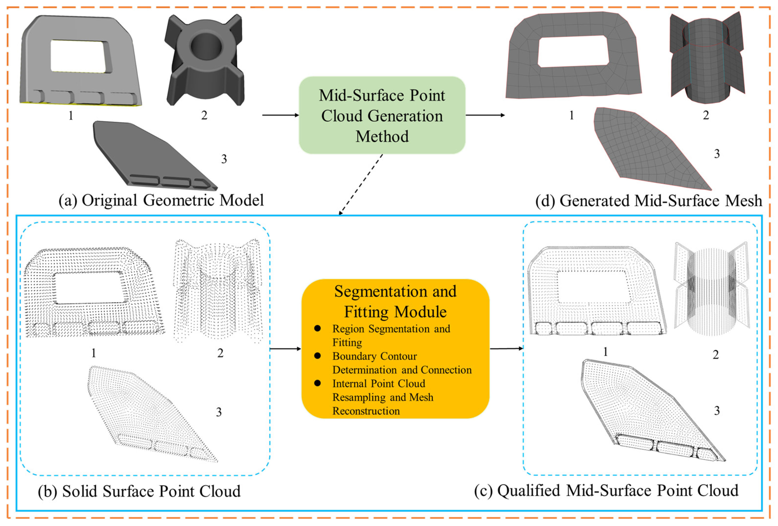
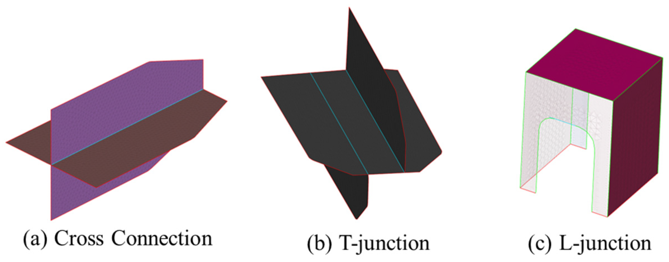
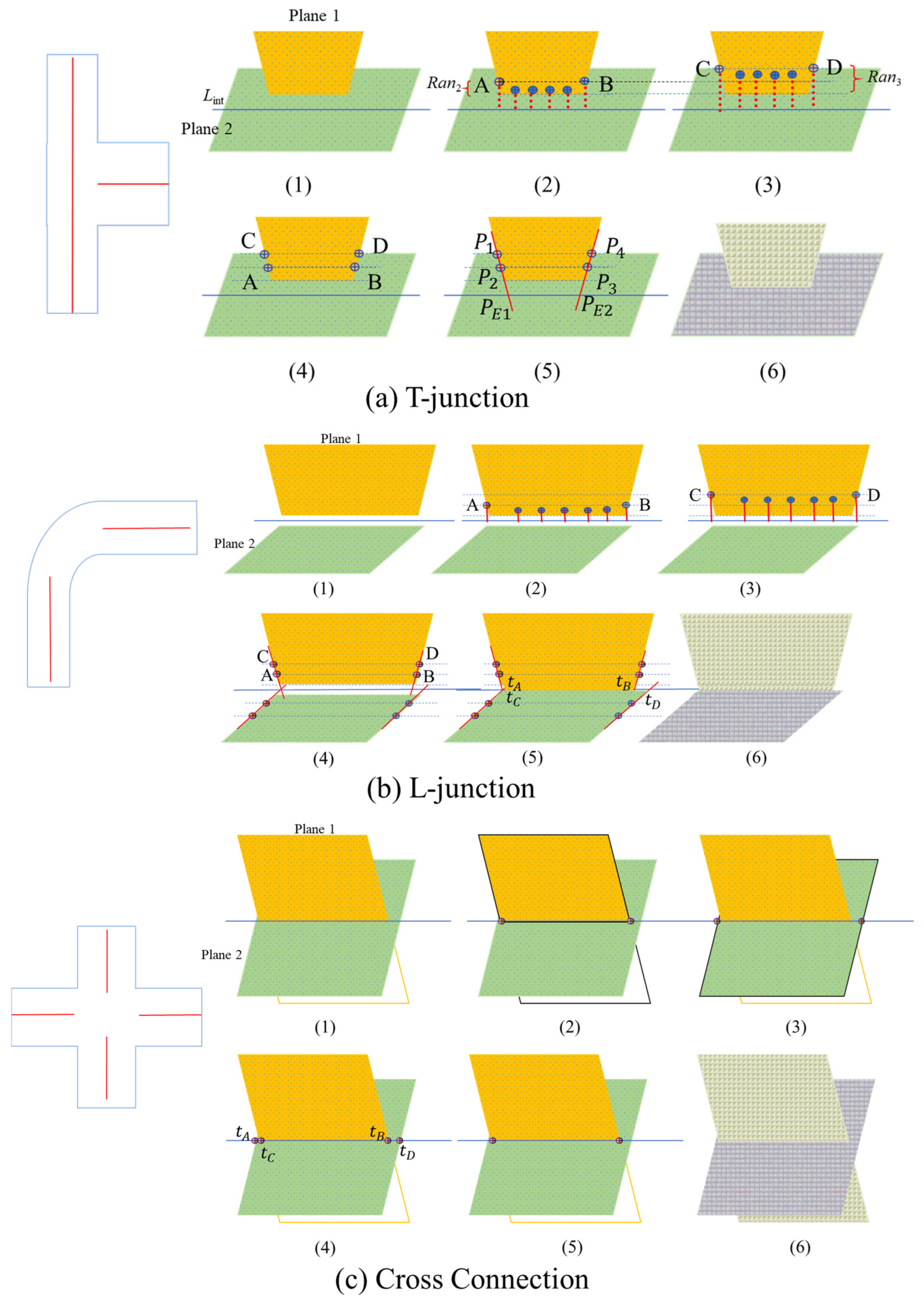
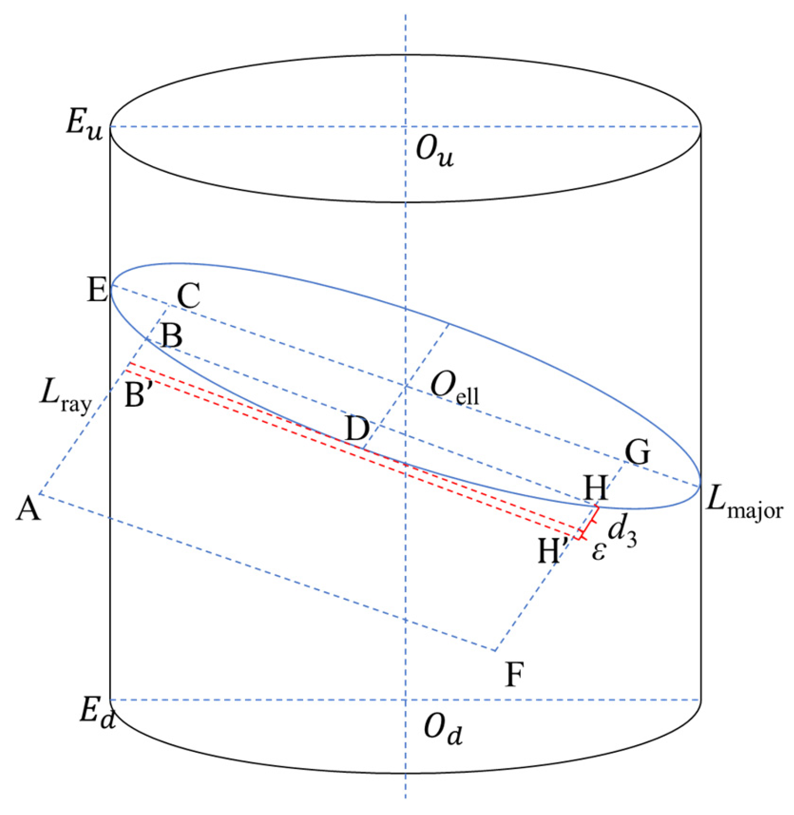
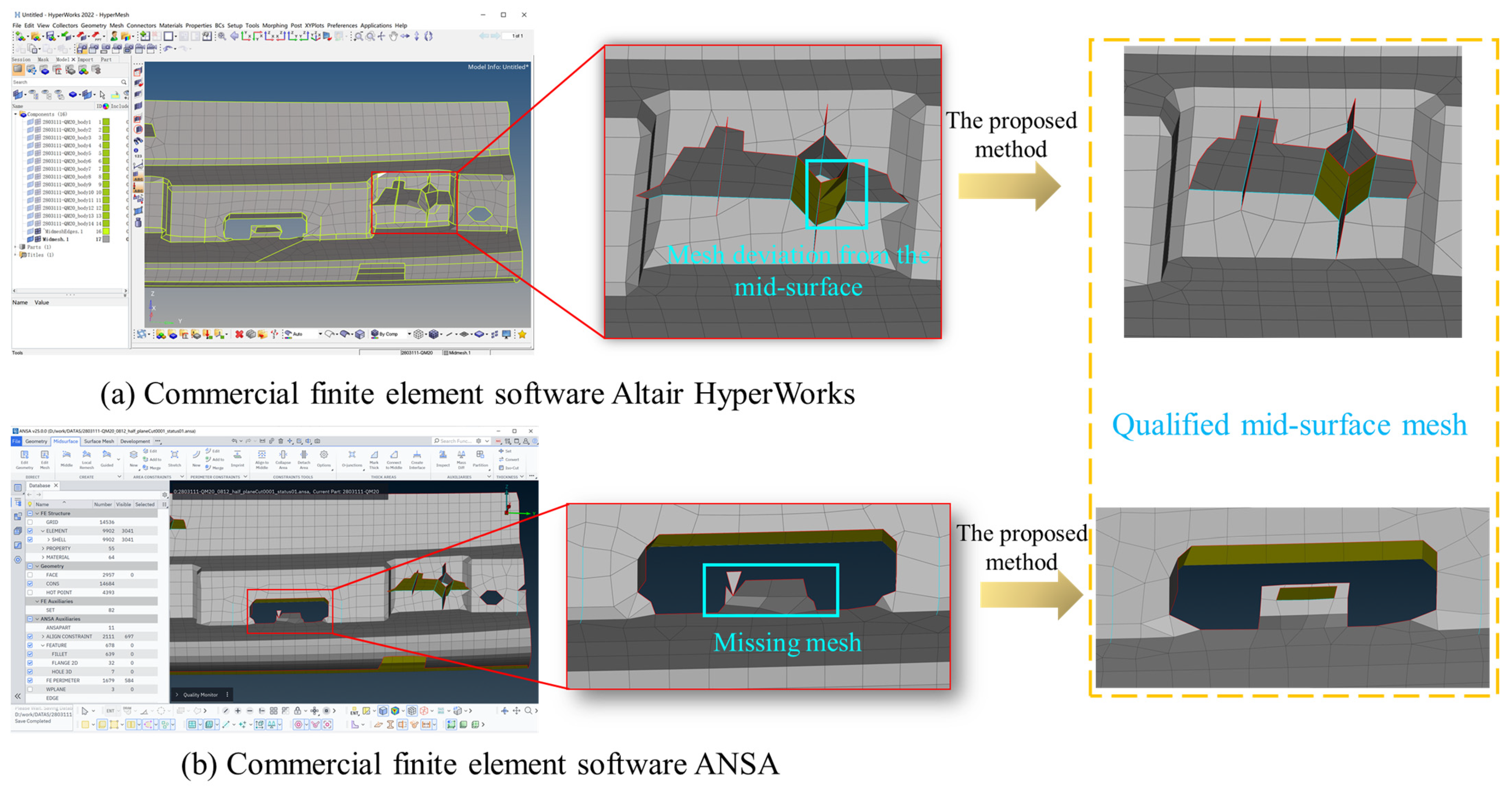
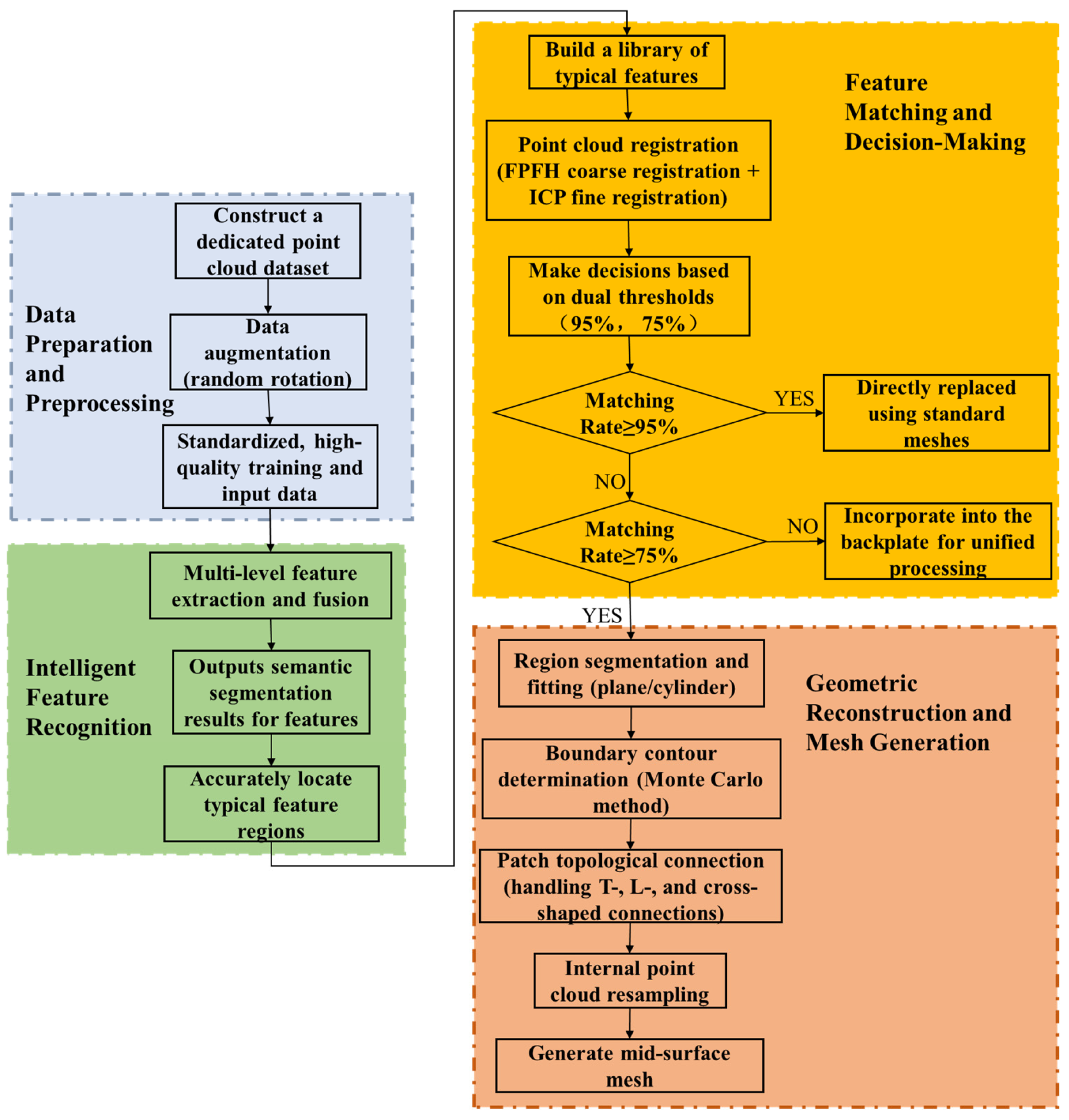
The proposed automated mesh generation method for automotive plastic parts is founded on a technical architecture comprising three core modules: (1) an AI-based intelligent feature recognition module, (2) a point cloud registration module, and (3) a segmentation-fitting mid-surface generation module.

In the first module, semantic segmentation is performed on the input point cloud using the PointNet++ model, enabling the intelligent classification and localization of typical features such as clips and backing plates (Section 2). The second module involves the construction of a standard feature library for plastic parts. Through feature-level point cloud registration, direct mesh replacement is applied to regions that successfully match the pre-defined templates (Section 3). For features exhibiting low registration confidence, the third module adopts a segmentation-fitting algorithm to reconstruct the mid-surface geometry. The generated surfaces are subsequently integrated to form a globally consistent and high-quality mesh (Section 4).

By fully automating the workflow—encompassing feature recognition, registration matching, and mid-surface generation—the proposed method achieves both high precision and high efficiency in constructing mid-surface meshes for plastic parts. The overall technical framework of this study is illustrated in Figure 1.

Accurate recognition of typical features, such as clips and backing plates, in automotive plastic parts constitutes a critical prerequisite for automated mid-surface mesh generation. The primary challenges in this task are as follows: (1) plastic parts are typically thin-walled, small in scale, and geometrically diverse; (2) features such as clips and backing plates exhibit considerable variations in dimension and curvature, making unified modeling difficult using conventional approaches; and (3) local features often share high topological similarity, which frequently leads to misclassification.

To address these challenges, a dedicated point cloud dataset of automotive plastic part features is constructed in this study, and an AI-based recognition module is developed using an enhanced PointNet++ architecture. The module performs feature-level semantic segmentation on input point clouds, thereby establishing a reliable geometric-semantic foundation for subsequent automated mesh generation.

2.1. Construction of the Automotive Plastic Part Feature Dataset

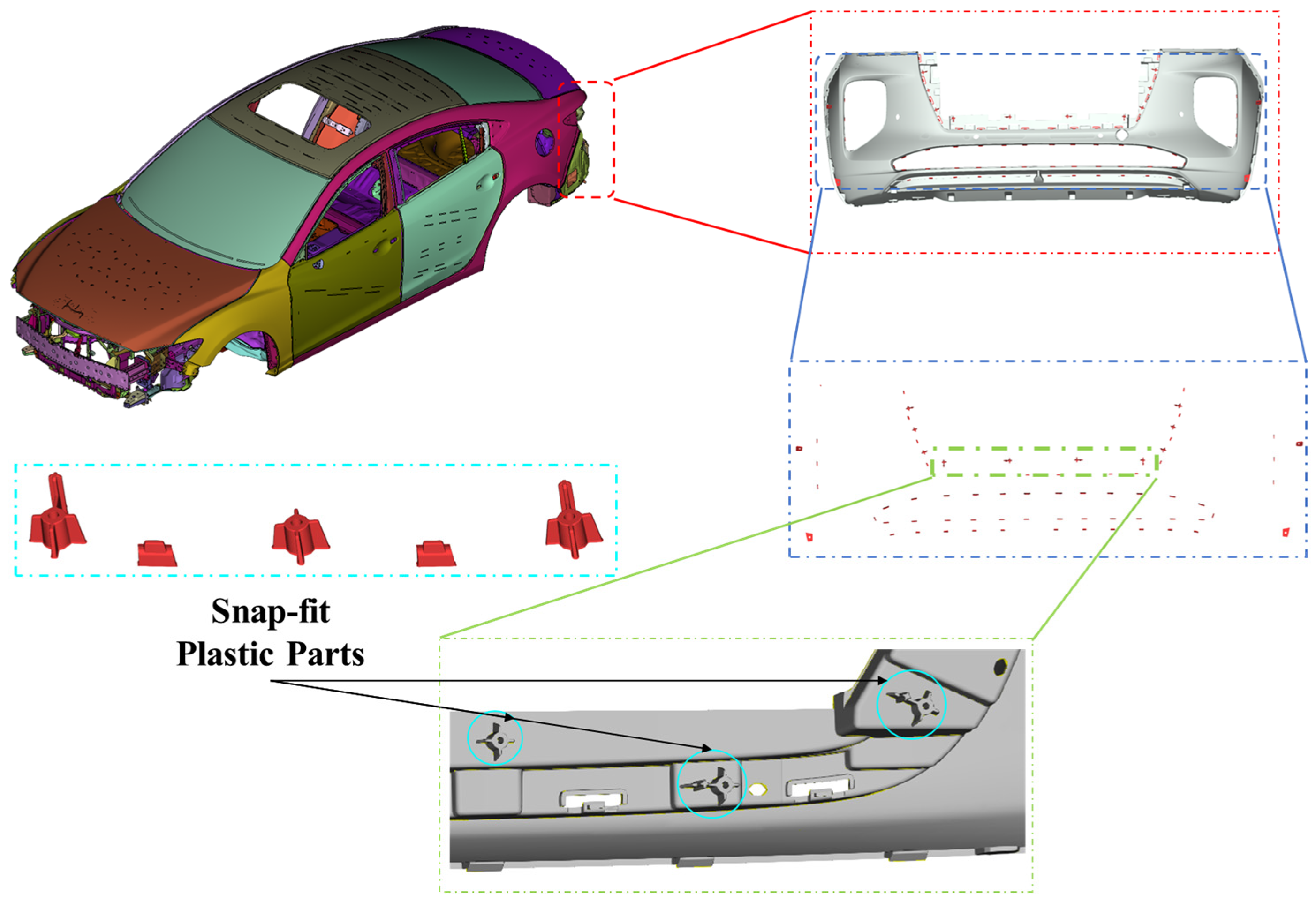
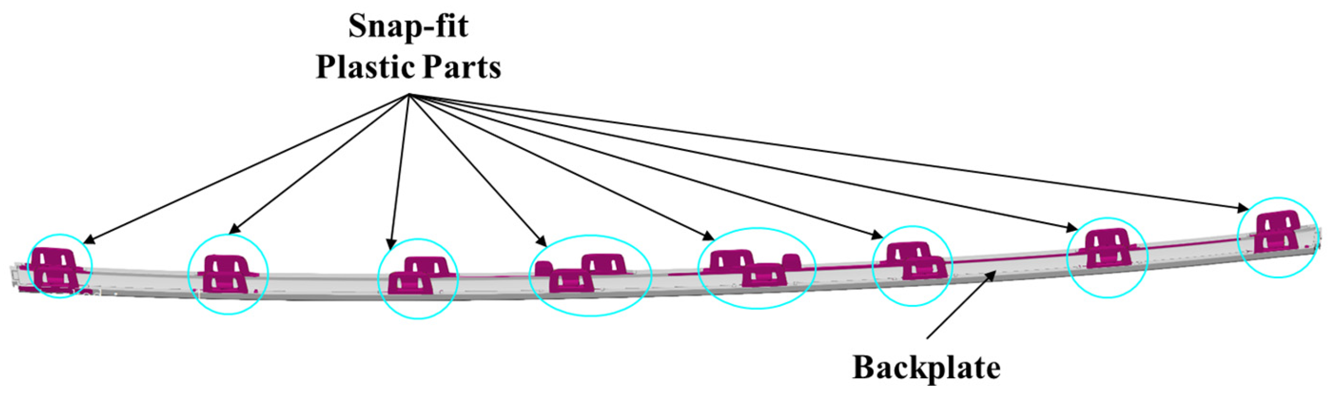
Due to the absence of annotated datasets for typical features of automotive plastic parts in publicly available resources, a dedicated point cloud dataset was constructed in this study. The dataset comprises three-dimensional coordinates, normal vectors, and semantic labels for each point. Based on differences in structural function and morphology, the typical features are categorized into two main classes: plastic clips and backing plates, as illustrated in Figure 2.

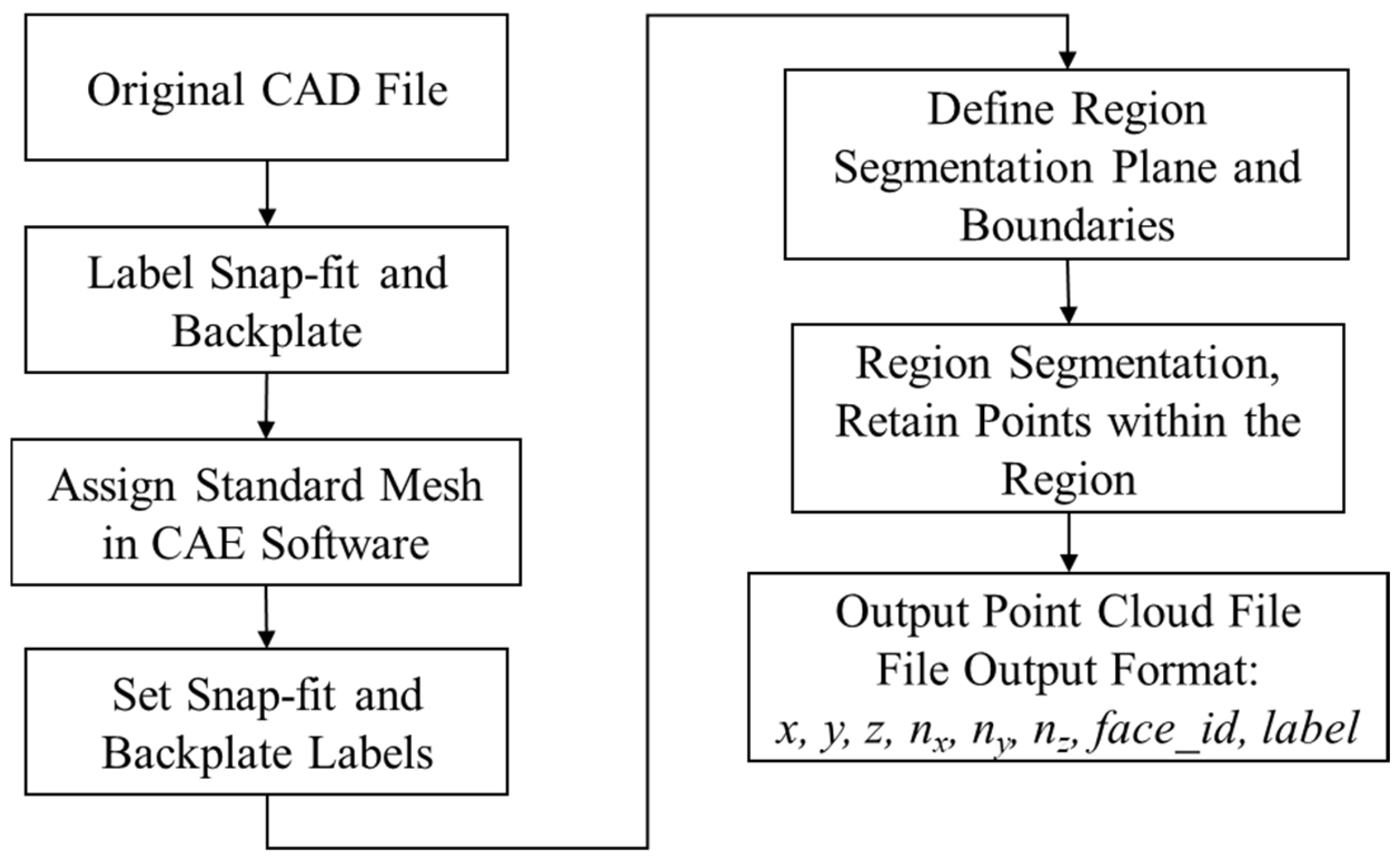
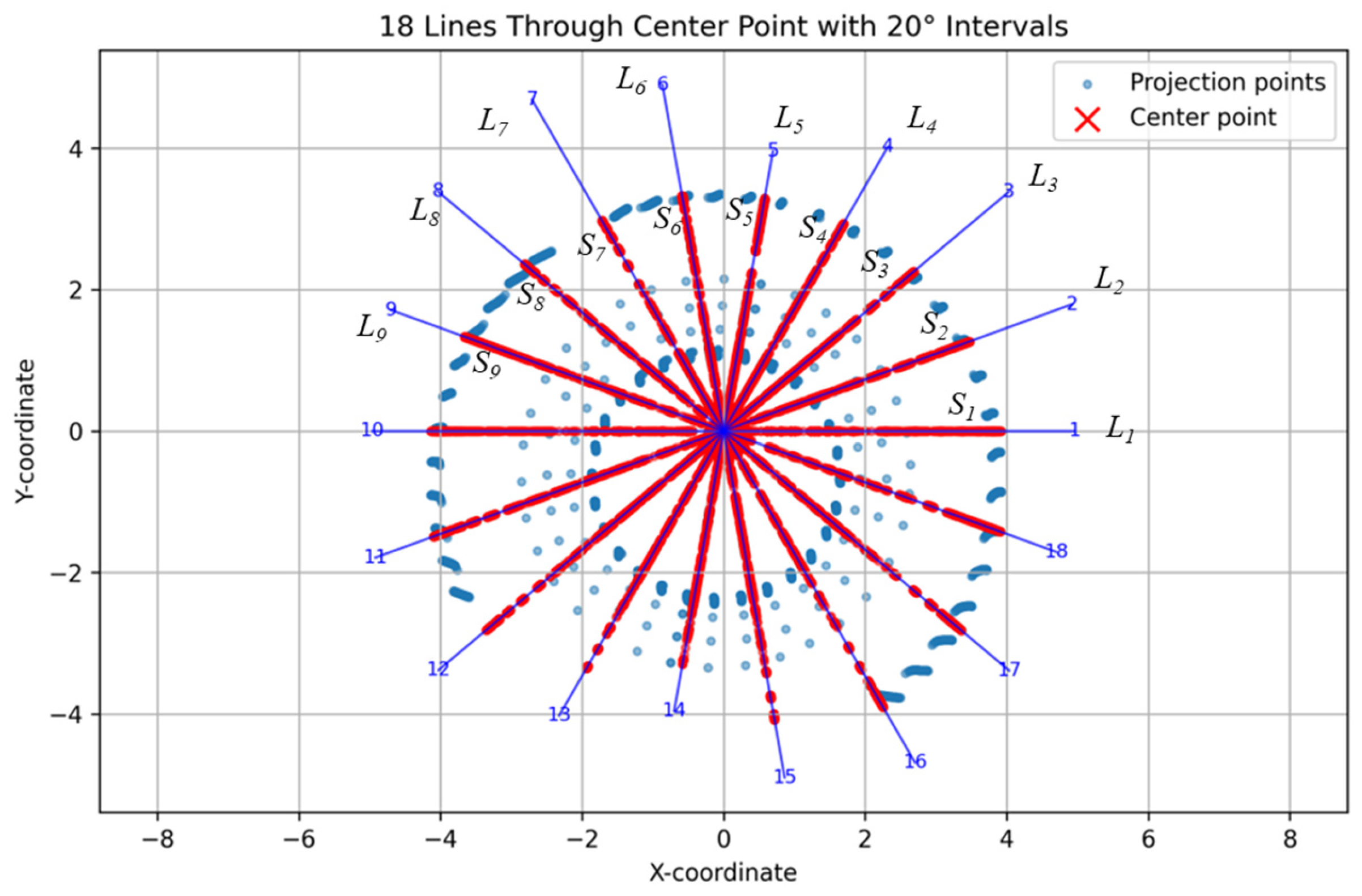
To improve the efficiency and consistency of dataset construction, a fully automated workflow was developed, starting from original geometric models. As shown in Figure 3, the procedure involves the following steps. Initially, all geometric files stored in a specified directory are traversed. Each file undergoes mesh generation and quality control to produce a structure suitable for point cloud extraction. Subsequently, key attributes, including centroid coordinates, normal vectors, face identifiers, and classification labels, are automatically retrieved from the mesh elements. Finally, an intelligent algorithm selects an optimal projection direction for region partitioning and exports the point cloud data in TXT format according to predefined standards, ensuring that each file satisfies the required point count and data dimensionality for subsequent processing.

It is worth noting that due to the large size of the original components, the geometric models were segmented into smaller blocks during dataset construction to adequately capture fine features such as clips. In the dataset derived from ten vehicle models, the clip label was designated as 50 and the backing plate label as 51. The complete dataset comprises 132,000 samples, aggregated from the ten models, including instances containing only backing plates. After 16 rounds of systematic model iteration and dataset quality optimization, the optimal model was ultimately identified. Notably, this model was not trained on the full expanded dataset of 132,000 samples but rather on a carefully curated subset consisting of samples with “at least one intact clip” (31,000 samples). This decision was validated through multiple comparative experiments.

Parallel training and testing were conducted on three derived datasets, namely, “only intact clips,” “at least one intact clip,” and “full dataset with backing plates removed.” The “at least one intact clip” dataset demonstrated unique advantages. It preserves the real-world industrial scenario where clips and backing plates coexist, providing a foundation for contrastive learning between the two component types, thereby avoiding the lack of contextual relevance observed in the “only intact clips” dataset. Simultaneously, by enforcing the core condition of “at least one intact clip,” low-quality samples with severely damaged clips or ineffective features were effectively excluded. This mitigates the interference caused by such samples during model training, as encountered in the “full dataset with backing plates removed” configuration.

Table 1. Training version record.

Version Number	Training Version	Number of Datasets	mIoU	Recognition Rate
1	Base version (2 cars data)	5.6 w	0.8964	32.53%
2	A random angle is enhanced based on the base version	11.2 w	0.8528	53%
3	Based on the base version, 9 angles are randomly enhanced	56 w	0.8	19.27%
4	The base version removes the pure backplane data	1.8 w	0.8028	61.4%
5	The base version removes the pure backplane data and randomly enhances an angle	3.6 w	0.7971	56.63%
6	The basic version only retains the full snap	3612	0.8035	51.8%
7	The base version retains at least one full snap	9264	0.8549	60.7%
8	4 cars remove the back panel data	3.4 w	0.8170	73.4%
9	Only 4 cars retain their full buckles	1.2 w	0.8558	71.3%
10	4 cars retain at least one complete buckle	1.4 w	0.8533	42.8%
11	6 cars remove the back panel data	5.1 w	0.7755	63.6%
12	Only 6 cars retain their full buckles	1.6 w	0.8523	49.3%
13	6 cars retain at least one complete buckle	2.7 w	0.8679	68.2%
14	10 cars remove the back panel data	9.3 w	0.8006	75.5%
15	Only 10 cars retain their full buckles	2.1 w	0.8436	56.12%
16	10 cars retain at least one complete buckle	3.1 w	0.8461	80.17%

presents a comprehensive record of the iterative model development process and serves as an ablation study to validate the design choices. To investigate the impact of dataset composition, a series of comparative experiments was conducted by training models on various data configurations. First, models trained on the raw dataset (Version 1) were compared against those trained after the removal of pure backing plate data (Versions 4, 8, 11, and 14). The substantial improvement in recognition accuracy, for instance, from 32.53% in Version 1 to 61.4% in Version 4, demonstrates that eliminating redundant, non-discriminative samples is essential for effective feature learning.

Furthermore, an ablation study on feature completeness was performed by contrasting models trained exclusively on “only complete clips” (Versions 6, 9, 12, and 15) with those trained on samples containing “at least one complete clip” (Versions 7, 10, 13, and 16). The results indicate that the “at least one complete clip” strategy, adopted in the final model (Version 16), achieves the optimal balance. This configuration benefits from the simultaneous presence of both clips and backing plates, facilitating contrastive learning, while effectively excluding severely incomplete samples that could otherwise degrade model performance.

The final optimized dataset, comprising 31,000 samples with at least one complete clip, was randomly partitioned into training (80%), validation (10%), and test (10%) sets. The class distribution in the test set is approximately balanced with respect to the point counts for clips and backing plates, reflecting real-world application scenarios.

Moreover, to account for pose variation in real scanning scenarios, a data augmentation strategy based on random 3D rotation was applied. Specifically, random rotation matrices about the x-, y-, and z-axes were generated and used to synchronously transform both point coordinates and their associated normal vectors. This approach simulates different placement angles and viewing perspectives without increasing the volume of physical data, thereby reducing the risk of pose-specific overfitting and enhancing the model’s capacity to learn intrinsic geometric features.

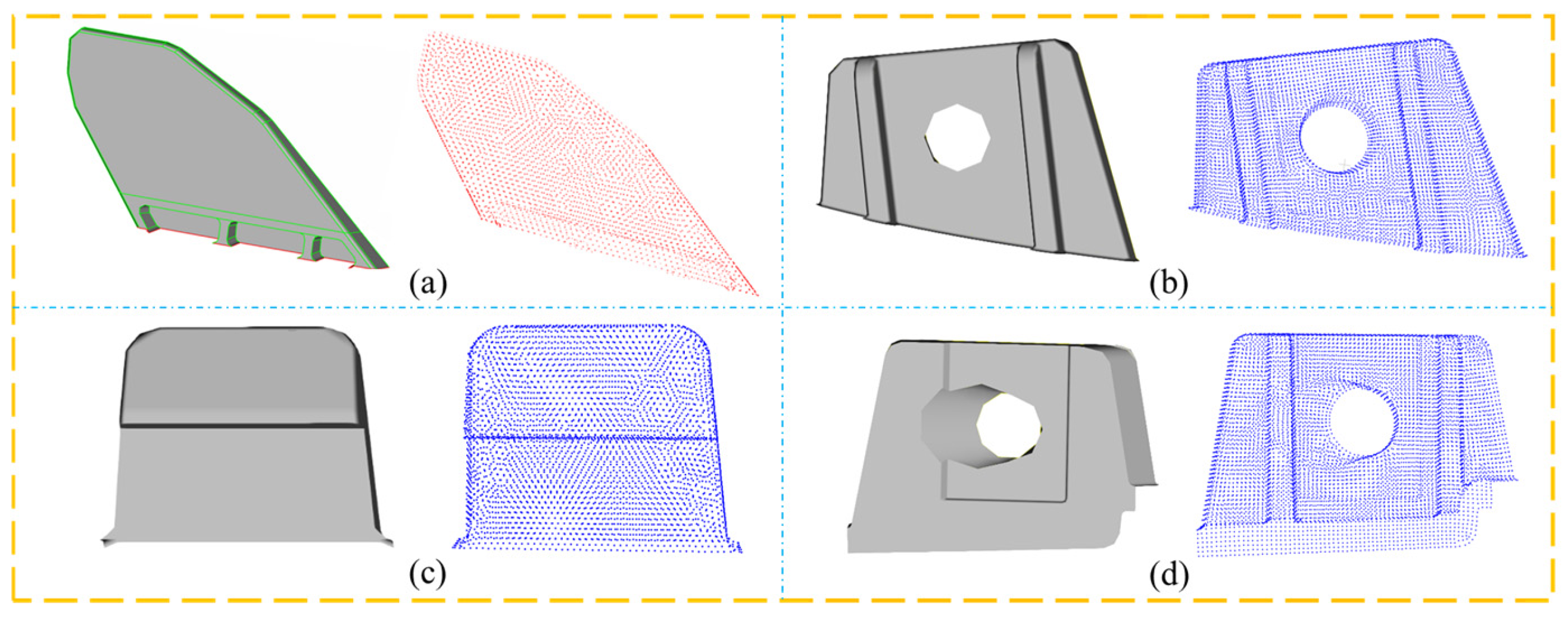
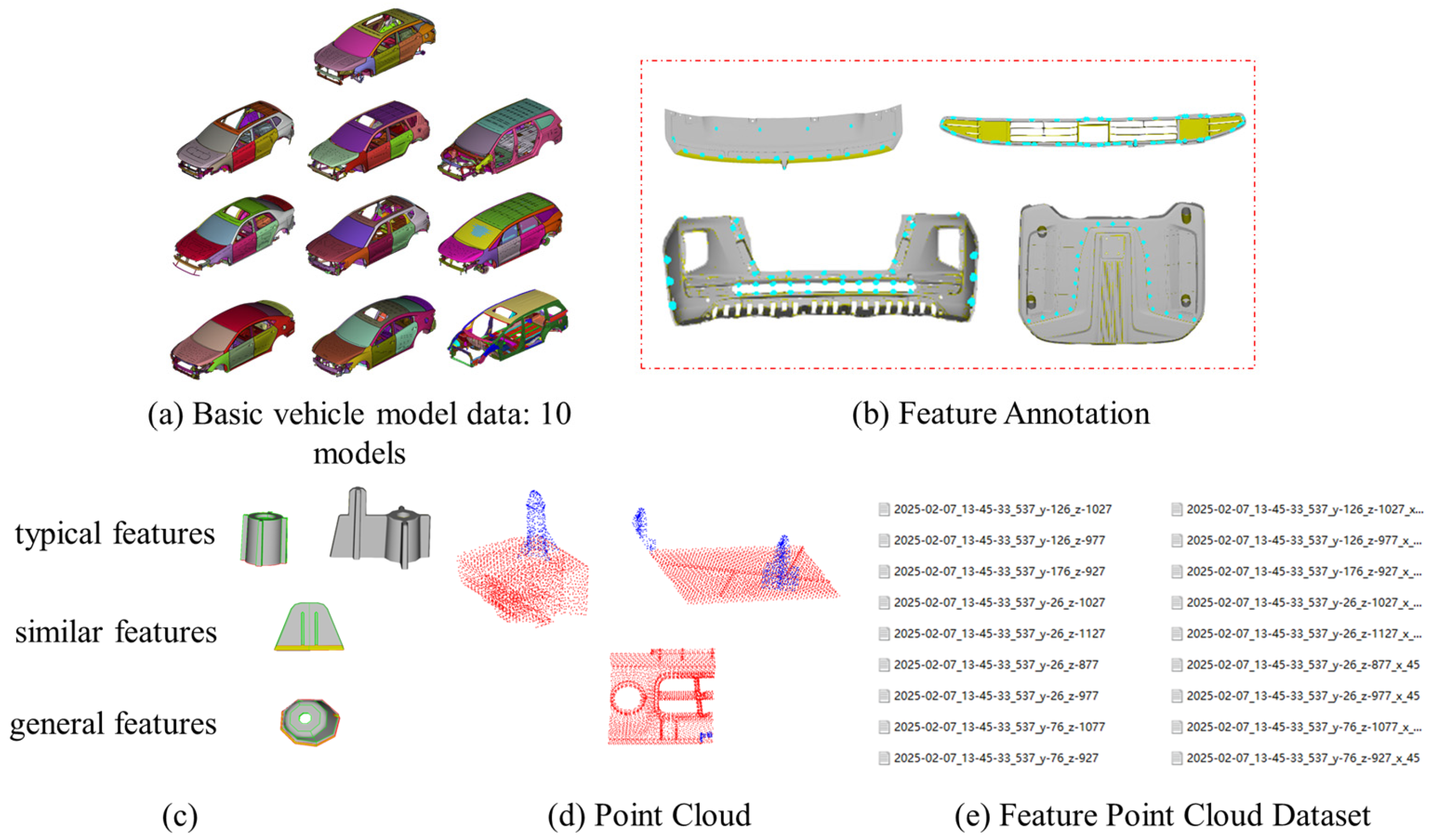
Following the methodology described above, a specialized point cloud dataset comprising 132,000 samples was constructed, as illustrated in Figure 4. This dataset provides a high-quality foundation for subsequent feature recognition and mesh generation tasks.

2.2. Plastic Part Feature Recognition Model Based on PointNet++

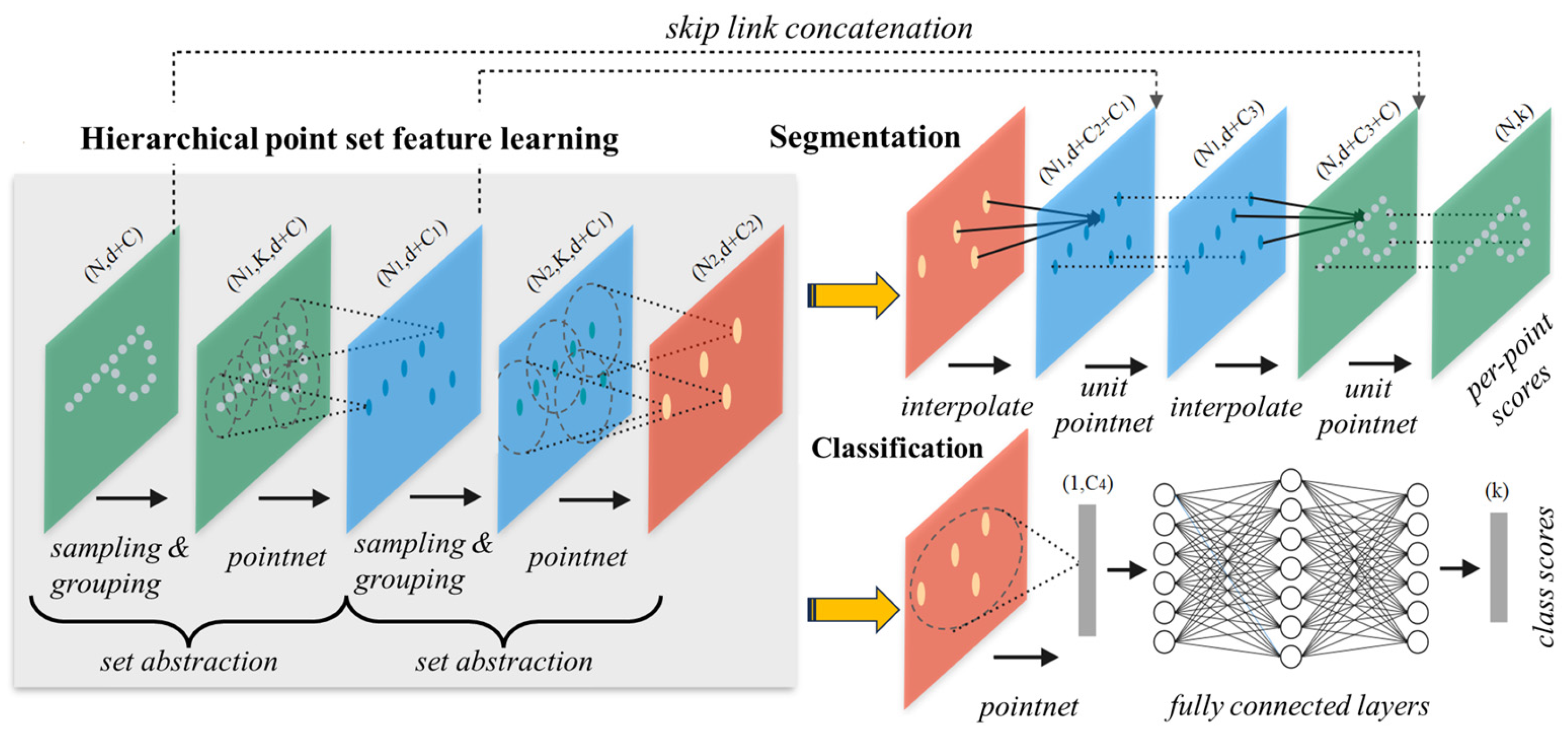
To address the complex local geometry and detailed features characteristic of plastic parts, PointNet++ is adopted as the feature recognition model in this study, as illustrated in Figure 5 [31]. In contrast to PointNet, the PointNet++ architecture progressively expands the receptive field through a hierarchical procedure of sampling, grouping, and feature extraction. This approach effectively integrates local geometric details with global semantic information, thereby enhancing its capability to capture intricate local features. A systematic model training framework was developed based on the PointNet++ architecture, with targeted improvements in three aspects: data preprocessing, training process control, and parameter optimization.

(1)

Data Preprocessing

To eliminate variations in point cloud scale and spatial position, input point clouds were first normalized through two specific steps: coordinate centering and scale normalization. Coordinate centering was performed by computing the mean of each coordinate dimension and translating the geometric center of the point cloud to the origin, thereby removing positional offsets introduced by different scanning setups. Scale normalization was subsequently applied to fit the entire point cloud within a unit sphere based on the maximum distance from the origin. This process mitigates interference caused by dimensional differences, for instance, clip lengths varying between 5 and 15 mm, enabling the model to focus on geometric morphology rather than absolute size and thereby improving cross-sample generalization.

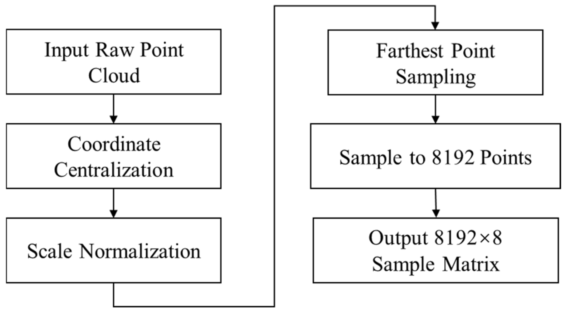
To satisfy the fixed-dimensional input requirement of the model, a farthest-point sampling strategy was employed to uniformly sample each point cloud frame to 8192 points. It was determined that 1024 points were insufficient to adequately characterize clip details given their size variation. In this method, an initial point was randomly selected, and subsequent points were iteratively chosen as the farthest from the existing set until the target number was reached. During sampling, the 3D coordinates, normal vector, and class label of each point were preserved, resulting in a sample matrix of size 8192 × 8, as shown in Figure 6. This ensures a standardized input format with complete feature information.

(2)

Training Process Control

During training, the number of input points per sample and the feature extraction levels were both set to 16. The input point clouds were processed through three Set Abstraction (SA) modules for hierarchical feature extraction:

In SA Layer 1, 2048 points were sampled with a neighborhood radius of 0.05. After being processed by an MLP with dimensions of 64 → 128 and max-pooling, a 256-dimensional feature was output, capturing local details such as clip edges and backing plate textures.

In SA Layer 2, 512 points were sampled with a radius of 0.1. Following transformation by an MLP (128 → 256), a 512-dimensional feature was generated, encoding medium-scale structural relationships.

In SA Layer 3, 128 points were sampled with a radius of 0.2. After processing through an MLP (256 → 512), a 1024-dimensional feature was obtained, representing global semantics.

Each SA operation followed the workflow of sampling, neighborhood query, feature transformation, and aggregation, progressively increasing the level of feature abstraction. Subsequently, Feature Propagation (FP) layers were employed to restore high-level features to the original point cloud resolution via trilinear interpolation using the three nearest neighbors. The 1024-dimensional global feature was first upsampled to 512 points and concatenated with the corresponding feature from SA Layer 2, forming a 1536-dimensional vector. This vector was further upsampled to 2048 points and concatenated with the SA Layer 1 feature (256-dimensional) and the original 6-dimensional geometric features (coordinates and normals), resulting in a final 1798-dimensional feature vector. Through the use of skip connection mechanisms, the model achieves deep fusion of multi-level features, preserving the semantic discriminative power of high-level features while integrating geometric details from low-level features. This provides a robust foundation for subsequent precise segmentation.

To further improve the accuracy of segmentation boundaries, negative log-likelihood loss was adopted as the optimization objective. This loss function assigns greater weight to misclassified points, particularly those in transition regions between clips and backing plates, thereby reinforcing the model’s learning on difficult samples and effectively enhancing boundary segmentation precision.

To ensure training stability and mitigate overfitting, a combination of performance monitoring and regularization techniques was applied. Every five epochs, classification accuracy, precision, recall, and F1-score were evaluated on both the training and validation sets, with loss and accuracy curves visualized, as shown in

Table 2. Per-class segmentation performance of the optimized PointNet++ model on the test dataset.

Class	Precision	Recall	F1-Score	IoU
Clip (Label 50)	0.82	0.79	0.80	0.81
Backplate (Label 51)	0.89	0.91	0.90	0.88
Overall	-	-	-	0.8461 (mIoU)

. Dropout was introduced between the SA and MLP layers to reduce neuron co-adaptation, and an L2 regularization term was added to the optimizer to constrain parameter magnitudes.

(3)

Parameter Optimization

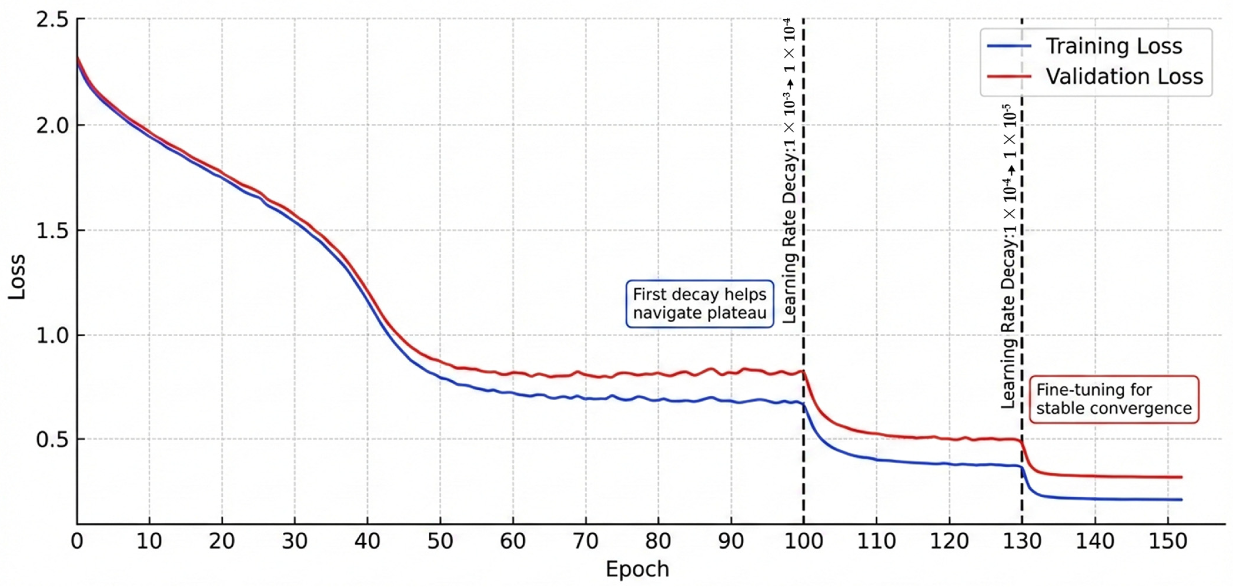
The model was updated via backpropagation using the Adam optimizer. Gradients were computed layer by layer from the loss layer, encompassing MLP weights, convolution kernels, batch normalization parameters, and bias terms, thereby ensuring effective gradient propagation to the input. The hyperparameters of the Adam optimizer were set as β₁ = 0.9, β₂ = 0.999, with an initial learning rate of 1 × 10⁻³. A piecewise decay schedule was applied, reducing the learning rate to 1 × 10⁻⁴ at epoch 100 and further to 1 × 10⁻⁵ at epoch 130, as shown in Figure 7. This strategy enabled rapid convergence in the early stages, with loss decreasing by more than 60% within the first 50 epochs, while facilitating stable fine-tuning in later phases, thereby mitigating gradient vanishing or oscillation and promoting robust convergence to an optimal state. Upon completion of training, the network weights were saved in a .pth file.

Regarding the evaluation of feature recognition performance, a comprehensive assessment was conducted from two perspectives: segmentation accuracy and engineering usability.

Mean Intersection over Union (mIoU) reflects the overlap between predicted and ground-truth regions, with higher values indicating more precise segmentation.

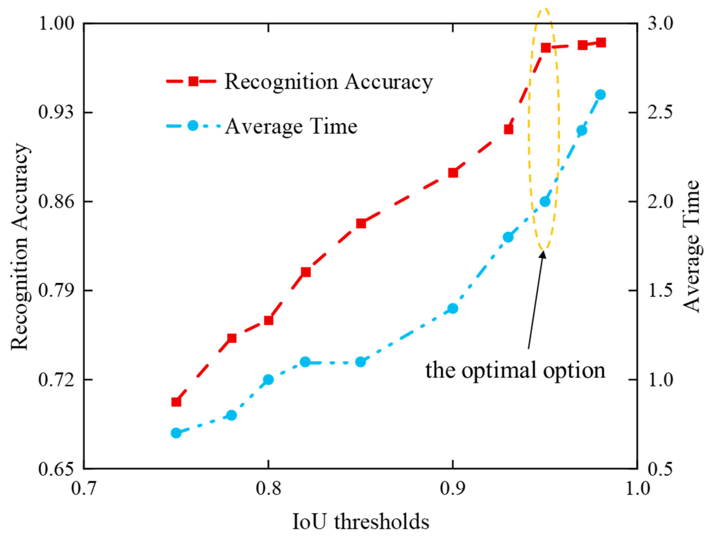
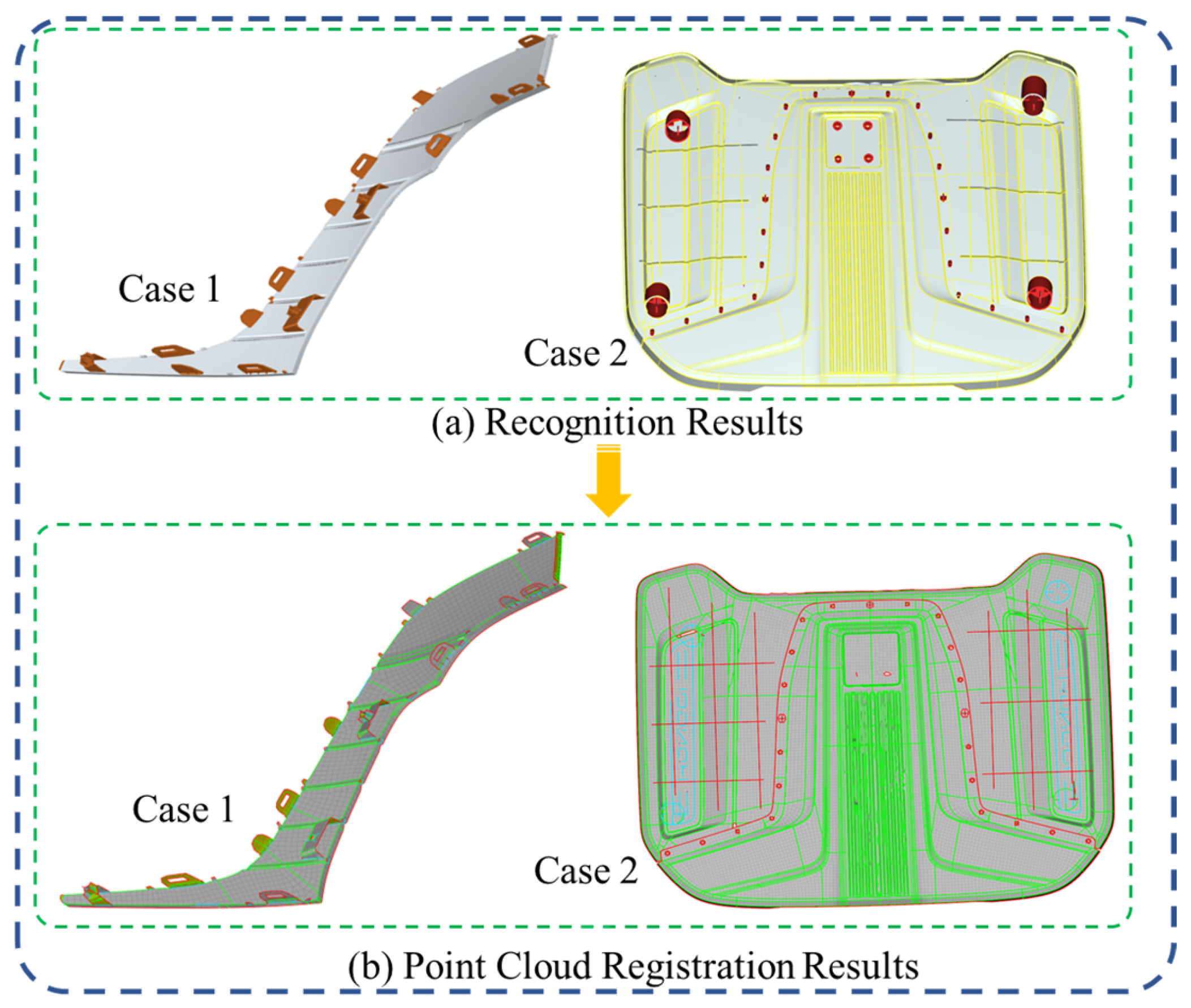
Visual Recognition Accuracy was assessed by deploying the trained model within a CAE software environment. Unlabeled point clouds, containing only coordinates, normals, and face IDs, were input into the model, and the recognized clip regions were highlighted in the CAE interface based on point-to-face mapping. Engineers then visually compared these regions with the original geometry to compute a practical accuracy rate. This evaluation emphasizes the method’s effectiveness for deployment in real industrial scenarios. The visual recognition result is shown in Figure 8.

3. Point Cloud Registration Module

To address the practical requirements of vehicle development, where the reuse of platform components and the introduction of new design configurations often coexist, a point cloud registration module is introduced. This module is designed to match recognized part features with standardized mesh templates, thereby improving processing efficiency while maintaining modeling quality.

The module operates through a sequential workflow. First, a library of typical plastic clip features is constructed based on engineering expertise to serve as a reference for registration. Next, a matching algorithm is employed to search the library and identify the source point cloud most similar to the newly recognized clip. Finally, a predefined matching-rate threshold is used to determine whether an existing template mesh can be directly reused or whether the model should be routed to the subsequent segmentation-fitting pipeline. This approach effectively balances geometric consistency with computational efficiency.

3.1. Construction of the Typical Feature Library

The typical feature library serves as a core component of the point cloud registration module. Its construction follows three guiding principles: representativeness, generality, and distinctiveness. Representativeness requires that the selected features either appear frequently in plastic parts or possess highly similar variants. Generality ensures that the corresponding mid-surface meshes for these features are adaptable to most structures of the same type, with consistent element sizing maintained for direct replacement. Distinctiveness demands clear differentiation in overall or local geometric morphology among different features to guarantee uniqueness within the library.

Based on these principles, a feature library was constructed from 10 basic vehicle models. The library comprises 102 categories, containing a total of 1132 distinct clip template meshes and their corresponding point clouds, representing the most commonly used clip designs in automotive engineering practice. In the matching process, each target clip undergoes a coarse-to-fine registration against all source point clouds in the library. The runtime complexity of this process is approximately O (K * M * log M), where K denotes the library size and M represents the number of points in a point cloud. To accelerate the search, a KD-tree structure was employed for nearest neighbor searches during the ICP fine registration stage. For the current library size, the entire matching process for a single target clip requires less than 0.5 s. To accommodate scaling to larger libraries, strategies such as approximate nearest neighbor (ANN) search can be readily incorporated; this direction is planned for future exploration to further enhance scalability.

A set of typical clip features was selected, as illustrated in Figure 9. For each feature, the point cloud generation process outlined in Section 2 was applied to obtain its geometric point cloud data (the source point cloud) along with a corresponding high-quality mid-surface mesh. This yields a paired “point cloud–mesh” data unit. All such paired units collectively constitute a structured, typical feature library, establishing the foundation for subsequent matching operations.

3.2. Feature Library Matching

Using the clip point cloud segmented by the aforementioned PointNet++ model as the target point cloud, and the point clouds stored in the feature library as source point clouds, the feature library matching module systematically evaluates the matching quality between each target and the source candidates. Through a screening process, the module identifies the source point cloud that best corresponds to the target geometry. This is achieved via a coarse-to-fine registration pipeline.

In the coarse registration stage, an initial alignment is performed using the Fast Point Feature Histogram (FPFH) descriptor. After voxel downsampling with a voxel size of 1.0, FPFH features are extracted from both point clouds. These features are used to compute an initial transformation matrix, denoted as T_coarse, which brings the source and target point clouds into rough alignment.

In the fine registration stage, starting from the coarse alignment result, the Iterative Closest Point (ICP) algorithm is applied to iteratively refine the registration. This stage minimizes the point-to-plane distance residual, yielding a precise transformation matrix, T_icp. The overall transformation between the source and target point clouds is then obtained as the composition of the coarse and fine alignment results:

$$T_{final}=T_{icp}\ast T_{coarse}.$$

(1)

The registered point cloud pair is recorded.

To quantify registration quality at each iteration of the point cloud alignment process, the spatial overlap between the two point clouds is evaluated using voxel occupancy, with the Intersection over Union (IoU) serving as the similarity metric. Adapted to the characteristics of the research objects in this study, the procedure is implemented as follows:

First, dimensionality reduction via voxelization converts the continuous spatial distribution of the point clouds into discrete grid-occupancy statistics. After merging all coordinate points from the two registered point clouds, a minimum coordinate offset is applied to ensure all points reside in the positive coordinate region.

As shown in

Table 3. Validation of choice of voxel size.

Voxel Size	Recognition Accuracy	Average Time
0.5	99.2%	35 s
1.0	98.7%	32 s
1.5	96.3%	27 s
2.0	95.3%	19 s
2.5	84.8%	13 s
3.0	72.3%	10 s

, when the voxel size increases to 2 mm, the recognition accuracy already exceeds 95%. However, achieving further improvement in recognition accuracy would require a further reduction in voxel size, which leads to a substantial increase in processing time, a trade-off that is not worthwhile.

Hence, a voxel size of 2 is set, and the coordinates of each point are discretized into integer voxel indices based on this size. Through offset and rounding operations, voxelization is completed. The resulting voxel sets for the target and source point clouds are denoted as V_tar and V_src, respectively. Next, 3D voxel indices are mapped to unique 1D identifiers, and Boolean occupancy vectors are generated to indicate whether each voxel is occupied by the corresponding point cloud.

Second, through Boolean operations, the number of voxels jointly occupied by both point clouds is counted, denoted as the intersection voxel count intersection $\left|V_{tar}\cap V_{src}\right|$. The total number of voxels occupied by either point cloud is counted, denoted as the union voxel count $\left|V_{tar}\cup V_{src}\right|$. The 3D IoU similarity is then calculated as

$$3D IoU={\displaystyle \frac{\left|V_{tar}\cap V_{src}\right|}{\left|V_{tar}\cup V_{src}\right|}}.$$

(2)

This metric ranges from [0, 1]. A higher value indicates greater spatial distribution overlap and stronger geometric feature consistency between the two point clouds.

Through a dynamic comparison mechanism, automatic screening of the optimal source point cloud matching result is achieved. For each target point cloud, the feature library is traversed, and the match with the highest similarity is retained, realizing automatic selection of the optimal source point cloud.

3.3. Main Screening Mechanism

During the evaluation and classification stage, the overlapping region between the target point cloud and a source point cloud is regarded as the matched area. A Boolean matching mask is generated to label all matched points. The matching rate is defined as the ratio of the number of matched points to the total number of points in the source point cloud, with values ranging from 0 to 1. A higher matching rate indicates greater geometric similarity between the target clip and the corresponding reference clip in the feature library.

As illustrated in Figure 10, the recognition accuracy and average processing time were evaluated under varying matching rate thresholds. The results indicate that a threshold of 0.95 yields a recognition accuracy exceeding 99.2% while maintaining a reasonable average processing time, as it ensures near-perfect geometric correspondence for the direct replacement path. Lowering the threshold to, for example, 0.94 leads to a noticeable decline in the mesh qualification rate due to the inclusion of geometrically mismatched features that cannot be faithfully represented by the template meshes. Conversely, raising the threshold above 0.97 would unnecessarily route many well-matched clips to the more computationally expensive segmentation-fitting path without significant quality improvement. Therefore, the 95% threshold is empirically validated as the optimal balance between accuracy and efficiency. The lower bound of 75% was established as the point below which features exhibit substantial dissimilarity (matching rate < 75%) and are better processed integrally with the backing plate; this decision is further supported by the sensitivity analysis.

Based on the matching results, a dual-threshold mechanism is employed to determine the subsequent processing path, as follows:

High similarity (Matching Rate ≥ 95%): The standard mid-surface mesh associated with the source point cloud is directly applied as a replacement.

Moderate similarity (75% ≤ Matching Rate < 95%): The segmentation-fitting algorithm described in Section 4 is invoked to generate a newly adapted mid-surface mesh.

Matching failure (Matching Rate < 75%): Features in this category—typically large or structurally special—are either processed together with the backing plate or flagged as requiring no independent processing.

For features with a matching rate below 75%, it is considered that no standard template has been successfully matched. In many cases, these features correspond to either very large clips or geometrically unique structures that are unsuitable for independent mesh generation. In the current pipeline, such features are routed to the “Belongs to Backing Plate” path. Algorithmically, this means that their segmented point cloud is not passed to the subsequent clip-specific processing modules, namely, mesh replacement or segmentation-fitting. Instead, these points are retained as part of the main backing plate point cloud and processed together with the surrounding base surface. The mid-surface mesh for these regions is generated as an integral part of the larger, continuous surface of the backing plate during the overall surface reconstruction process.

This simplification carries important engineering implications. While it ensures that the automated pipeline can handle all cases without failure, it may compromise the geometric fidelity and mechanical accuracy of these non-standard but potentially critical clips. If such a clip serves as a primary load-bearing or fastening feature, modeling it as part of the continuous backing plate could lead to inaccuracies in stress distribution or assembly simulation. Therefore, this path is intended as a safe fallback for non-critical features or as a temporary placeholder. Future work will aim to enhance the feature library and segmentation-fitting algorithms in order to reduce the number of clips that fall into this category.

This screening mechanism enables fully automated routing while ensuring the geometric quality of the resulting mesh.

4. Segmentation-Fitting Mid-Surface Generation Module

For clips with a matching rate in the [75%, 95%) interval (Section 3.3), the following segmentation-fitting pipeline is applied. This module is also applicable to challenging cases, such as incomplete cylindrical data and complex boundary topologies.

4.1. Region Segmentation and Fitting

Clip structures are typically composed of planar and cylindrical regions. To achieve accurate region localization, a pipeline involving segmentation, culling, partitioning, fitting, and projection is adopted. First, based on predefined spatial rules, such as segmentation along the x- or y-axis, the clip and its associated mid-surface point cloud are divided into several sub-regions. This step reduces the scale of point clouds processed at one time and improves computational efficiency. Next, curvature analysis is performed to identify and remove “fillet points,” which are points located in high-curvature transition zones that do not belong to valid planar or cylindrical fitting regions. This removal minimizes interference with the primary geometric fitting.

Subsequently, the filtered point cloud is clustered into multiple candidate planar patches using spatial connectivity. Patches formed by noise or edge artifacts are discarded, retaining only structurally complete patches. For each valid planar patch, a mid-surface plane equation is fitted using the least-squares method, and all points within the patch are orthogonally projected onto the fitted plane along their normal vectors. For cylindrical regions, the point cloud is projected onto a parametrically fitted cylindrical surface.

While planar fitting is relatively conventional and not elaborated upon here, traditional cylinder-fitting methods often depend on complete point cloud data and are sensitive to noise and missing regions, such as incomplete cylinders, frequently leading to axis-direction deviation and inaccurate center-point positioning. For cylindrical regions, we propose a robust fitting method that handles incomplete cylinders, as detailed below.

We take the eigenvector corresponding to the smallest eigenvalue as $\overrightarrow{a}$ (see Appendix A.1 for the full derivation).

To determine a point $\overrightarrow{r_0}$ on the axis, we project all surface points onto a plane perpendicular to $\overrightarrow{a}$. For an incomplete cylinder, the centroid of the projected points is biased. We correct this bias using a longest-chord and perpendicular-bisector strategy (Figure A1, Figure A2, Figure A3 and Figure A4). The detailed procedure is given in Appendix A.2.

Finally, we calculate the distance from all cylinder surface sample points to this axis and take the average as the final estimated value for the cylinder radius R.

Through the above workflow, high-precision, robust fitting of geometric parameters for both complete and incomplete cylinders is achieved, laying an accurate geometric foundation for subsequent mid-surface mesh generation.

4.2. Boundary Contour Determination and Connection

4.2.1. Precise Delineation of Boundary Contours

Following region segmentation and fitting, the precise delineation of each feature region’s boundary is essential for subsequent reverse modeling. Unlike convex hull or Alpha-shapes, our method handles non-convex and multi-hole boundaries without parameter tuning.

To address these issues, a randomized boundary determination method based on Monte Carlo simulation is proposed, adopting a “reverse empty-space filling” strategy. Through a distance-field filtering mechanism and dynamic threshold search, this method enables the direct and concurrent localization of boundary points. When combined with a centroid-based dynamic ray expansion strategy, it automatically classifies inner and outer boundaries, thereby accurately resolving complex topologies containing internal holes and establishing a foundation for subsequent point cloud reordering.

(1)

Point Cloud Dimensionality Reduction and Empty Space Identification

To reduce computational complexity, the 3D boundary extraction problem is first reduced to 2D plane processing. For a fitted plane equation,

$$Ax+By+Cz+D=0.$$

(3)

Its unit normal vector is defined as

$$\overrightarrow{n}=\left(A,B,C\right).$$

(4)

For a 3D point cloud set $P_{3D}=\left\{p_1,p_2,\dots ,p_n\right\}$, the projection point $p_i^{\prime }\left(x_i^{\prime },y_i^{\prime },z_i^{\prime }\right)$ of any point $p_i\left(x_i,y_i,z_i\right)$ onto the fitted plane can be obtained through geometric transformation:

$$p_i^{\prime }=p_i-\left(p_i·\overrightarrow{n}+D\right)\overrightarrow{n}.$$

(5)

Subsequently, by establishing a local coordinate system, the projection point $p_i^{\prime }\left(x_i^{\prime },y_i^{\prime },z_i^{\prime }\right)$ is mapped to 2D plane coordinates (u_i, v_i), obtaining a 2D point set $P_{2D}$. This projection transformation strictly preserves the topological connectivity of the original point cloud, ensuring consistency between 2D boundaries and 3D solid edges.

We then generate a large set of random points on the plane. A random point is marked as an “empty-space point” if its distance to the nearest projected point exceeds threshold r (Figure 11). This creates a “negative mold” of the solid region. Parameter settings are detailed in Appendix A.3.

(2)

Boundary Point Extraction and Classification

A boundary point is defined as a point in the original point cloud that can “touch” an empty space point. Since the filtering process creates a “vacuum band” with a width of approximately r between the solid edge and the empty space points, directly using radius r for neighborhood search would fail to find boundary points. Therefore, an extended search radius is introduced, calculated as

$$R_{se}=r+\delta ,$$

(6)

where δ is a system correction value. Boundary points are then identified using the extended search radius (Equation (6), Figure 12). The choice of δ is discussed in Appendix A.3.

To distinguish inner and outer boundaries, we check whether the ray from the geometric center to a boundary point intersects an empty-space island (Figure 13). The complete classification algorithm is given in Appendix A.3.

4.2.2. Topological Connection Between Patches

After boundary extraction, we reconstruct the topological skeleton between adjacent patches. A virtual boundary expansion strategy helps detect potential intersections. To reduce computational cost, only boundary points (not all interior points) are considered.

In practice, due to scanning inaccuracies and segmentation artifacts, logically adjacent patches may not be in physical contact. To address this issue, a virtual boundary expansion strategy is introduced. A base expansion step length, denoted as Δs, and a maximum expansion length, S_max, are predefined. Without altering the patch normal or the original point distribution, boundary points are iteratively extrapolated radially or along their normal direction. As the boundaries expand, adjacent patch boundaries eventually intersect, and these intersection points serve as candidates for identifying potential connection relationships.

Since patches are only defined by the plane Equation (3) and discrete boundary points, performing strict pairwise intersection tests for all patch pairs would incur massive computational cost. Therefore, the concept of spatial linear programming is introduced, utilizing half-space properties for rapid pre-screening. Assume two candidate planes: Plane 1 ($f_1\left(x\right)=A_{1}x+B_{1}y+C_{1}z+D=0$) and Plane 2 ($f_2\left(x\right)=A_{1}x+B_{1}y+C_{1}z+D=0$). Select any point P₁ (x₁, y₁, z₁) on the boundary of Plane 1 and substitute it into the equation of Plane 2 to obtain an algebraic discriminant (the scaled signed distance):

$$d_2=f_2(P_1)=A_2{x}_1+B_2{y}_1+C_2{z}_1+D_2.$$

(7)

As shown in Figure 14, if the two planes are completely separated in space and do not occlude each other, all boundary points of Plane 1 substituted into $f_2(x)$ should yield values of the same sign (e.g., all negative). This indicates that Plane 1 lies entirely in the negative half-space of Plane 2. During boundary expansion, if point P₁ crosses Plane 2, the sign of d₂ will flip. Once it is detected that within the boundary point set of Plane 1, there exists,

$$f_2(P_i)·f_2(P_j)<0,$$

(8)

then Plane 2 can be judged as a potential intersecting plane of Plane 1 and added to the intersection candidate pool for subsequent high-precision determination.

We then compute the theoretical intersection line L_int and verify the overlap of the projected boundary segments (Figure 15). Overshoot portions beyond the intersection line are trimmed based on a geometric threshold (Figure 16).

Based on the relative positions and angular differences between the normals of adjacent planar patches, their topological relationships are categorized into two primary types: merge and intersect.

When two planes satisfy the strict intersection criterion and the angle between their normal vectors is less than 10°, they are classified as merge. In this case, the intersection line is not computed; instead, the corresponding point clouds are directly merged, and a new plane equation is fitted to eliminate segmentation-induced gaps.

When the angle exceeds 10°, the relationship is classified as intersect. Depending on the spatial distribution of the point clouds, three specific topological configurations are further distinguished: Cross connection, T-junction, and L-junction, as illustrated in Figure 17.

Besides intersections between planes, connections between planes and cylindrical surfaces are common in plastic parts (e.g., ribs connecting to cylindrical holes). Let the plane equation be f₁, the cylinder axis equation be L_axis, and the radius be R. Calculate the Euclidean distance d_c from any point p_i on the plane boundary to the cylinder axis:

$$d_c={\displaystyle \frac{‖{\overrightarrow{n}}_{cy1}\times \left({\overrightarrow{r}}_{p_i}-{\overrightarrow{r}}_0\right)‖}{‖{\overrightarrow{n}}_{cy1}‖}},$$

(9)

where ${\overrightarrow{n}}_{cy1}$ is the cylinder axis vector and ${\overrightarrow{r}}_0$ is a point on the axis. If d_c > R, the plane is outside the cylinder, and there is no intersection line. Otherwise, the plane and cylinder are judged to intersect. The intersection line is typically an elliptical arc or hyperbola, which can be analytically obtained by solving the system of plane and cylinder equations.

For a T-junction, the intersection line extent is constrained by the rib width; endpoints are recovered via layered sampling (Figure 18a). Detailed parameter settings are given in Appendix A.4.

For L-junction and Cross Junction

Given that L-junctions and Cross-junctions share a common geometric characteristic, the effective range of the intersection line must simultaneously fall within the geometric projection intervals of both Plane 1 and Plane 2. Therefore, the core task involves solving the intersection of two one-dimensional parameter intervals, as illustrated in Figure 18b,c.

Let the direction vector of the infinite intersection line L_int be $\overrightarrow{v}$. Any point on the line can be represented as

$$P\left(t\right)=P_0+t·\overrightarrow{v}.$$

(10)

First, calculate the effective parameter intervals of Plane 1 and Plane 2 on the intersection line:

$$\left\{\begin{array}{l}{R}_1=\left[t_A,t_B\right]\\ R_2=\left[t_C,t_D\right]\end{array}\right..$$

(11)

Compare the four endpoint parameters {A, B, C, D}, and the final intersection line range R_final is taken as the intersection of R₁ and R₂. If there is no overlap, it is judged that no valid intersection line exists.

For a plane-cylinder intersection, the intersection curve is an elliptical arc. We analytically compute the major axis and determine the minor-axis vertices using distance correction (Figure 19). Detailed derivations are provided in Appendix A.4.

4.3. Internal Point Cloud Reordering and Mesh Reconstruction

After obtaining the boundaries and topological skeleton, the original interior point cloud may be unevenly distributed. Direct triangulation would produce poor-quality meshes. Therefore, we regularize the interior point cloud using a boundary-constrained dynamic circle envelope.

Accordingly, a mesh reconstruction algorithm based on boundary-constrained interior-point guidance is proposed. This algorithm utilizes the precisely determined boundaries to define an envelope space and treats the original interior points as “geometric seeds.” Through a dynamic radius constraint mechanism, uniformly distributed interior mesh points are generated and filtered, ultimately achieving complete and high-quality patch reconstruction. The specific procedure consists of the following steps.

(1)

Local Coordinate Transformation and Envelope Space Construction

Using the fitted plane equation, we transform the patch to a local 2D coordinate system (u, v). Denote the transformed boundary point set as B_2D and the original interior point set as I_2D. Traverse the boundary point set B_2D to determine its extrema in the u and v directions: u_min, u_max, v_min, v_max. The transformed boundary points define a bounding box Ω:

$$\Omega =\left[u_{\min },u_{\max }\right]\times \left[v_{\min },v_{\max }\right].$$

(12)

(2)

Generation of Regular Candidate Point Set

Within Ω, based on the set reordering step size δ (determining final mesh resolution, typically 0.5 mm or 1.0 mm), generate a regular grid candidate point set:

$$\begin{array}{l}{G}_{cand}=\left\{g_{ij}\right\}\\ g_{ij}=\left(u_{\min }+i·\delta ,v_{\min }+j·\delta \right)\end{array},$$

(13)

where I and j are indices. This set includes points inside the patch, in outer voids, and near boundaries, requiring further screening.

(3)

Definition of Valid Region Based on “Dynamic Circle Envelope”

To precisely define the valid region of the patch, a “dynamic circle envelope” algorithm is introduced, using the original interior points (“seed points”) I_2D = {p₁, p₂, …, p_n} as geometric priors. A perception circle C_k is constructed centered on each seed point p_k, with its radius r_k dynamically determined based on the distance from that point to the boundary:

Set a relatively large base search radius R_base (suggested to be 1.5~2 times the reordering step δ). For each seed point p_k, calculate its shortest Euclidean distance d_min to the boundary:

$$d_{\min }\left(p_k\right)=\underset{b\in B_{2D}}{{\displaystyle \min }}‖p_k-b‖.$$

(14)

If d_min > R_base, this indicates that the seed point is far from the boundary, located in the central area of the patch (safe zone); then, set r_k = R_base. Otherwise, the seed point is close to the boundary (edge zone). To prevent the perception circle from overflowing beyond the boundary, set

$$r_k=d_{\min }\left(p_k\right)-\epsilon ,$$

(15)

where ϵ is a small safety margin, ensuring the circle is tangent to or inside the boundary. Through this mechanism, the connected domain formed by all perception circles closely adheres to the inner side of the boundary, completely covering the solid region of the patch.

(4)

Valid Interior Point Screening and Final Point Cloud Merging

For each candidate grid point g_ij in the set candidate G_cand, perform an inclusion test:

$$Valid(g_{ij})=\left\{\begin{array}{ll}True,\hfill & \hspace{0.17em}\exists k,s.t.‖g_{ij}-p_k‖\le r_k\hfill \\ False,\hfill & \hspace{0.17em}otherwise\hfill \end{array}\right..$$

(16)

If it falls within any valid perception circle (i.e., condition (16) is true), it is judged as a valid interior point. After screening, obtain the valid interior reordered point set G_valid. To avoid adhesion to boundary points, points in G_valid that are too close to the boundary (e.g., distance < 0.5δ) are removed. Finally, merge the precise boundary point set B_final with the screened interior point set G_valid to form the patch’s final point cloud P_final.

(5)

3D Mesh Generation

After obtaining the final merged point cloud P_final in the 3D global coordinate system, the last step is to generate the surface mesh. In this work, a standard Delaunay triangulation algorithm was applied to the reordered and uniformly distributed point set. This step transforms the organized point cloud into a high-quality, regular-shaped patch mesh model, which serves as the final, simulation-ready mid-surface mesh for the plastic part feature. Finally, we apply Delaunay triangulation to P_final to produce the mesh.

5. Verification and Discussion

5.1. Mesh Quality Evaluation Metrics

To quantitatively evaluate mesh quality, the criteria widely adopted in the automotive CAE industry are employed, with reference to the guidelines provided by ANSYS Design Modeler, version 2023 R2. The key metrics and their corresponding acceptance thresholds for shell elements are defined as shown in

Table 4. Element Quality Inspection Standard.

Element Quality Metrics	Quality Requirements
Jacobian	≥0.7
Aspect Ratio	≤5
Minimum Angle (Triangle)	≥20°
Maximum Angle (Triangle)	≤120°
Skewness	≤60°
Warpage	≤5°
Minimum Angle (Quadrilateral)	≥45°
Maximum Angle (Quadrilateral)	≤135°

. A clip mesh is considered qualified only if it satisfies all of the specified criteria.

The test data were derived from nominal CAD geometries (Section 2.1), assuming clean, complete point clouds to be typical after reverse-engineering reconstruction. The core problem we address is the algorithmic failure of existing CAE tools to handle fine features (clips, ribs, etc.) even on perfect CAD data; therefore, validation on CAD-derived point clouds is appropriate and directly relevant to industrial CAE pre-processing workflows. Validation on raw scanner data is left for future work. We have explicitly outlined this as a future research direction in the Conclusions.

5.2. Typical Case Verification

5.2.1. Validation with Two Cases from the Original Models

To validate the effectiveness and practical applicability of the proposed mesh generation method, tests were performed on a dataset comprising plastic parts from ten vehicle models. In this dataset, clips and backing plates are assigned semantic labels 50 and 51, respectively. The dataset contains a total of 132,000 samples, including instances of pure backing plate data.

In terms of intelligent recognition performance, the model achieved a mean Intersection over Union (mIoU) of 0.8461 on the test set. This metric directly reflects the regional matching accuracy of point cloud segmentation, indicating an overlap of 84.61% between the model-predicted clip regions and the ground-truth regions, well above the industrial qualification threshold of 0.75. Furthermore, through interactive visual verification conducted in the CAE software ANSA, engineers compared the model-identified clip regions with the original geometry within the software interface. The resulting practical recognition accuracy for clips was measured at 80.17%, confirming that the segmentation output is directly applicable in engineering practice.

Figure 20 illustrates the clip recognition results for two representative cases, denoted as Case 1 and Case 2. Detailed registration results for each clip are provided in Appendix B. In summary, for Case 1, 11 clips achieved a matching rate ≥ 95% (direct replacement), and 3 clips fell into the 75–95% range (segmentation fitting). For Case 2, 26 clips were directly replaced, 4 clips had matching rates < 75% and were processed with the backing plate, and none required segmentation fitting.

Statistically, 90.9% of the samples in the dataset enabled all clips to be fully identified. For these fully identified clips, the point cloud registration method was applied to directly replace them with standard mid-surface meshes retrieved from the feature library. For clips that were not matched in the library or exhibited insufficient matching rates, the segmentation-fitting algorithm described in Section 4.2 and Section 4.3 was employed to generate the corresponding mid-surface meshes.

Figure 21a illustrates the complete workflow and output of the segmentation-fitting module for three plastic clips from Case 1 (matching rates between 0.75 and 0.95), from raw point cloud to final mesh. The process begins with the raw point clouds extracted from the clip’s solid surfaces (Figure 21b). After being processed by the proposed algorithm, a topologically correct mid-surface mesh model is produced (Figure 21d). The key intermediate steps and results, shown in Figure 21c, demonstrate the robustness and advantages of the method:

(1)

Planar and Cylindrical Feature Fitting

For regions identified as planar, the algorithm reliably performs normal- and distance-constrained query pairing, followed by least-squares fitting, to accurately locate their mid-surfaces. For structures containing cylindrical features (see label 2), high-precision parameter fitting is achieved. Even for relatively complete cylinders, fitting accuracy can be further improved through appropriate corrections.

(2)

Contour Recognition and Topology Construction

As indicated by label 1, the algorithm accurately identifies patch boundaries and inner and outer contours, effectively handling features such as internal holes and ensuring geometric completeness. More importantly, it automatically infers and constructs spatial topological connections between different patches, such as plane-cylinder interfaces, overcoming the isolation of fitted patches caused by local point cloud gaps or noise.

(3)

Intersection Line Calculation and Regularized Mesh Generation

Based on the established topology, the algorithm precisely calculates the valid range of intersection lines and generates corresponding connection point clouds, enabling seamless stitching between different geometric elements. Finally, through an internal point cloud regularization and reordering strategy, the initially projected unordered points are converted into a uniformly distributed grid. This approach fundamentally avoids low-quality mesh artifacts, such as holes or distortion, that may arise from direct triangulation, resulting in high-quality mid-surface meshes.

Figure 21. Final mid-surface mesh generation effect display for three plastic clips in Case 1 with matching rates between 0.75 and 0.95.

Figure 21. Final mid-surface mesh generation effect display for three plastic clips in Case 1 with matching rates between 0.75 and 0.95.

For a comprehensive comparison, a comparative analysis was performed between meshes created manually using professional CAE software and those generated automatically by the proposed method, as illustrated in Figure 22a,b. The manually produced meshes frequently exhibited quality defects such as fragmentation, distortion, and multiple disconnected faces. In contrast, the meshes generated by the proposed method demonstrated markedly superior quality.

The proportion of clips with qualified meshes was employed as a quantitative metric for evaluation, and the statistical results are presented in

Table 5. Mesh Qualification Rate and Time Comparison for Case 1.

Method	Number of Clips with Qualified Mesh	Total Clips	Clip Qualification Rate	Time Required to Generate Qualified Mesh
CAE Software	10	14	71.43%	2 h
Proposed Method	14	14	100%	36 min

and

Table 6. Mesh Qualification Rate and Time Comparison for Case 2.

Method	Number of Clips with Qualified Mesh	Total Clips	Clip Qualification Rate	Time Required to Generate Qualified Mesh
CAE Software	13	30	43.33%	6 h
Proposed Method	26	30	86.66%	1.8 h

. Experimental results demonstrated that the application of the proposed method improved mesh modeling efficiency by approximately 67%, while the mesh quality compliance rate increased sharply from 52.27% to 90.9%.

Furthermore,

Table 7. Comparison of mesh quality metrics between manual and automated methods for Cases.

Element Quality Metrics	Method	Ratio of Non-Conforming Elements
Jacobian	Manual	0.75%
	Proposed	0.51%
Aspect Ratio	Manual	0.42%
	Proposed	0.53%
Minimum Angle (Triangle)	Manual	0.84%
	Proposed	0.71%
Maximum Angle (Triangle)	Manual	0.68%
	Proposed	0.85%
Skewness	Manual	0.79%
	Proposed	0.24%
Warpage	Manual	0.61%
	Proposed	0.36%
Minimum Angle (Quadrilateral)	Manual	0.72%
	Proposed	0.64%
Maximum Angle (Quadrilateral)	Manual	0.55%
	Proposed	0.38%

presents the ratio of non-conforming elements for each metric, comparing manual and automated meshes across all test cases. It is worth noting that while Table 7 shows marginally higher ratios of non-conforming elements for Aspect Ratio and Maximum Angle (Triangle) in the proposed method compared to manual meshing, these differences are minor and well within acceptable engineering limits. In industrial CAE practice, a non-conforming element ratio below 5% is generally considered sufficient for reliable simulation results. The proposed approach delivers a highly favorable trade-off: it dramatically accelerates the pre-processing stage while maintaining—and in most metrics, exceeding—the quality of manually generated meshes. The slight variations in these two specific metrics do not undermine the practical utility of the method and are expected to be further reduced as the model continues to be refined with additional training data and further algorithmic improvements.

To rigorously evaluate the performance improvement achieved by the proposed method, statistical analyses were conducted on both processing time and mesh quality compliance rate across all ten vehicle models. A paired t-test and a Wilcoxon signed-rank test were performed to compare the manual workflow (using ANSA) with the automated method proposed in this study. The results are presented in

Table 8. Statistical Comparison of Modeling Time and Mesh Quality Between Manual (ANSA) and Proposed Automated Method Across Ten Vehicle Models.

Vehicle Model ID	Processing Time (Hours)		Mesh Quality Compliance Rate (%)
	Manual	Proposed	Manual	Proposed
Model 01 (Case 1)	2.0	0.6	71.43	100.00
Model 02 (Case 2)	6.0	1.8	43.33	86.66
Model 03	3.5	1.1	58.20	91.50
Model 04	4.2	1.3	62.80	92.30
Model 05	2.8	0.9	67.50	94.20
Model 06	5.1	1.6	51.40	88.70
Model 07	3.0	1.0	69.30	93.80
Model 08	4.8	1.5	55.60	89.40
Model 09	3.2	1.0	64.70	92.60
Model 10	5.5	1.7	48.90	87.50
Mean ± Std	4.01 ± 1.26	1.25 ± 0.38	59.32 ± 9.22	91.67 ± 4.08
p-value (paired t-test)	p < 0.001		p < 0.001
p-value (Wilcoxon)	p = 0.002		p = 0.002

.

The mean processing time was reduced from 4.01 h in the manual workflow to 1.25 h using the proposed method, corresponding to an average reduction of 68.8%. The paired t-test yielded a p-value of less than 0.001, and the Wilcoxon signed-rank test produced a p-value of 0.002. Both tests confirm that the observed reduction in processing time is statistically significant.

Regarding mesh quality, the mean compliance rate increased from 59.32% in the manual workflow to 91.67% with the proposed method. The paired t-test resulted in a p-value of less than 0.001, and the Wilcoxon signed-rank test yielded a p-value of 0.002. These results provide strong statistical evidence for the superiority of the proposed method in terms of mesh quality.

5.2.2. Generalization Across Unseen Vehicle Platforms

To further evaluate the generalization capability of the proposed method, two additional vehicle configurations (denoted as Vehicle A and Vehicle B) were tested, as illustrated in Figure 23. These two vehicles are completely different from the ten original models in terms of platform, clip designs, and overall geometry. Neither the PointNet++ model nor the feature library was exposed to any data from these two vehicles during training or library construction. The fully automated pipeline (PointNet++ segmentation → feature library registration → segmentation-fitting mesh generation) was applied to all clips on these two new vehicles.

Table 9. Performance comparison on unseen vehicle platforms (Vehicle A and Vehicle B).

Metric	Original Test Set (10 Vehicles, Held-Out Clips)	New Vehicle A	New Vehicle B
mIoU	0.846	0.833	0.828
Clip Recall	80.2%	79.1%	78.8%
Clip precision	0.82	0.81	0.80
F1-score	0.80	0.80	0.79
Mesh quality compliance rate	91.7%	89.2%	91.5%
Average processing time (per vehicle)	1.25 h	1.3 h	1.2 h
Time reduction vs. manual meshing	~67%	~67%	~68%
Jacobian	0.51%	0.53%	0.49%
Aspect Ratio	0.53%	0.55%	0.51%
Minimum Angle (Triangle)	0.71%	0.73%	0.69%
Maximum Angle (Triangle)	0.85%	0.87%	0.82%
Skewness	0.24%	0.26%	0.22%
Warpage	0.36%	0.38%	0.34%
Minimum Angle (Quadrilateral)	0.64%	0.66%	0.62%
Maximum Angle (Quadrilateral)	0.38%	0.40%	0.36%
High (≥95%)—direct mesh replacement	85%	83.4%	82.2%
Medium (75–95%)—segmentation-fitting	10%	11.1%	12.6%
Low (<75%)—belongs to backing plate	5%	5.5%	5.2%

summarizes the key results.

As shown in Table 9, the PointNet++ model trained only on the ten original vehicles maintained high segmentation accuracy on the two unseen platforms. The mIoU values were 0.833 (Vehicle A) and 0.828 (Vehicle B), compared to 0.846 on the original test set, while clip recall reached 79.1% and 78.8%, respectively, only slightly lower than 80.2%. These minor decreases are well within acceptable engineering tolerance and indicate strong generalization.

The mesh quality compliance rates on the two new vehicles were 89.2% and 91.5%, very close to the average of the original ten vehicles (91.7%). The average processing time remained consistently around 1.2–1.3 h, achieving the same dramatic efficiency improvement of approximately 67% compared to manual meshing. Detailed per-metric non-conforming element ratios (Jacobian, Aspect Ratio, etc.) are provided in the Table 9 and show no significant degradation.

In addition, the matching rate distribution against the existing feature library was evaluated. For Vehicle A, 83.4% of clips achieved a matching rate ≥ 95% (direct mesh replacement), 11.1% fell into the 75–95% range (segmentation fitting), and 5.5% had a matching rate < 75% (processed together with the backing plate). Vehicle B showed similar distributions (82.2%, 12.6%, and 5.2%, respectively). These results demonstrate that the proposed method generalizes well to entirely new vehicle platforms, with only minor performance degradation that remains within acceptable engineering tolerance.

5.3. Comparison with Existing Commercial Automated Mid-Surface Tools

To provide a complete picture, we also tested the built-in automatic mid-surface extraction functions of two widely used commercial CAE pre-processing tools (ANSA and Altair HyperWorks) on the same plastic part clips. The directly exported meshes suffered from severe fragmentation, missing clip features, and topological errors, as illustrated in Figure 24. In almost all cases, these meshes were not usable for downstream finite element analysis without extensive manual repair. For example, the mesh quality compliance rate of these raw automated outputs was below 5%, rendering a quantitative comparison against our method meaningless. Therefore, the only fair and practically relevant baseline is the manual/semi-automated workflow in ANSA after professional engineer repair, which represents the current industrial practice. Our method was compared against this baseline throughout the manuscript (Table 5, Table 6, Table 7 and Table 8), demonstrating a 67% reduction in processing time and an increase in mesh quality compliance rate from 59.3% to 91.7% on average.

5.4. Engineering Implications

The 67% reduction in labor time specifically targets one of the most tedious and repetitive aspects of a CAE engineer’s workflow: manual mesh repair and verification. As cited in the introduction, this task has been reported to consume up to 60% of total simulation time. Automating this routine, repetitive work is not intended to eliminate jobs, but rather to reallocate human capital toward higher-value tasks that genuinely require human ingenuity.

Currently, junior engineers often spend months or even years mastering the intricate and labor-intensive art of manual meshing. The proposed tool has the potential to significantly accelerate their learning curve by providing high-quality, validated starting meshes, thereby enabling them to focus on understanding the underlying physics, interpreting simulation results, and proposing design modifications. Consequently, they can transition from functioning as “mesh repair technicians” to becoming “simulation analysts” much earlier in their professional development.

For senior engineers, automation alleviates the burden of spending valuable time on checking and correcting meshes. This allows them to redirect their expertise toward addressing complex system-level challenges, innovating new simulation methodologies, and mentoring junior colleagues in strategic problem-solving.

It is important to emphasize that while the AI handles the repetitive, rule-based task of mesh generation, the engineer remains in full control throughout the process. The final mesh is always subject to the engineer’s review and approval before being employed in any simulation. The engineer retains the authority to override any automated decision, adjust parameters, or manually intervene when a highly unusual feature is encountered. Thus, the tool functions as an intelligent and efficient assistant, rather than an autonomous replacement. Automating the geometric construction enables the engineer to concentrate on the creative, analytical, and decision-making aspects of product development. This synergy between human intelligence and machine efficiency is essential for unlocking greater innovation and productivity in the engineering field.

6. Conclusions

To address the challenges of low efficiency and inconsistent quality in mid-surface mesh generation for automotive plastic parts, this paper proposed an automated method integrating deep learning-based feature recognition, point cloud registration, and segmentation-fitting techniques. The main conclusions are as follows:

(1)

A standardized point cloud dataset comprising 132,000 samples was constructed to accommodate the high geometric diversity and significant size variation observed in plastic part clips. By leveraging the hierarchical feature learning mechanism of PointNet++, the recognition challenges posed by large size differences and high topological similarity between clips and backing plates were effectively addressed. The optimized model achieved a mIoU of 0.8461, and its practical visual recognition accuracy reached 80.17%, both exceeding the industrial qualification threshold of 0.75. This performance overcomes the misclassification and missed detection issues commonly associated with traditional recognition approaches.

(2)

The proposed point cloud registration module, which combines a typical feature library, coarse-to-fine registration, and a dual-threshold screening mechanism, enables rapid feature-level mesh replacement. Validation results demonstrate that for clip features with matching rates above 95%, standard mesh replacement significantly improves modeling efficiency. For features with matching rates between 75% and 95%, the segmentation-fitting algorithm accurately restores the geometric morphology, ensuring adaptive processing across different similarity levels.

(3)

A series of optimized algorithms targeting clip mid-surfaces, cylindrical structures, and complex boundaries was proposed within the segmentation-fitting module. A cylinder parameter extraction method combining feature decomposition and geometric constraint correction improves fitting accuracy for incomplete cylinders. A Monte Carlo simulation-based strategy, coupled with dynamic ray expansion, achieves precise identification of inner and outer contours. Furthermore, a boundary-constrained point cloud reordering algorithm ensures mesh uniformity and topological integrity.

(4)

Experimental results confirm the engineering practicality of the proposed method. Compared with conventional approaches, the method reduces mesh modeling time by approximately 67% and increases the mesh quality compliance rate from 52.27% to 90.9%. Validation on two unseen vehicle platforms achieved compliance rates of 89.2% and 91.5%, with processing times consistently around 1.2–1.3 h, confirming strong generalization. The proposed approach addresses core difficulties in mid-surface mesh generation for plastic parts.

While the proposed method delivers significant improvements in both efficiency and quality, certain limitations remain. The efficiency of the point cloud registration module relies heavily on the comprehensiveness of the typical feature library. For entirely new clip designs not represented in the library, the matching rate will be low, routing them to the more computationally intensive segmentation-fitting module. Although this ensures geometric fidelity, it does not fully leverage the efficiency gains offered by mesh replacement. Therefore, the library requires ongoing maintenance and expansion to accommodate new designs.

Future work will focus on four areas: (a) deep generative models for automatic feature library expansion; (b) Transformer-based networks for improved semantic understanding; (c) validation on raw 3D scanned data with noise and warpage; and (d) downstream FEA validation to confirm the engineering impact of the generated meshes.