Rapid Physics-Based Synthesis of Diesel Engine Models for Hybrid Powertrain Optimization

Abstract

Concept-phase planning of diesel-engined hybrid vehicles requires rapid engine synthesis, including brake-specific fuel consumption (BSFC) estimation, with minimal input data. Fuel savings from hybridization arise partly through engine downsizing and engine-off operation, so trade studies depend on knowing the dependence of BSFC on engine sizing and speed and load conditions. This paper presents a method for synthesizing hypothetical modern diesel engines of any given size for the purpose of trade studies. The synthesized engines match the performance and efficiency capabilities of commercially available units. Relationships are developed between rated power, rated speed, peak torque, displacement and cylinder count for four vehicle application classes. Together with a BSFC estimation method, these relationships form a complete engine synthesis chain from rated power to a full torque curve and BSFC map. Known values may be substituted, such as minimum BSFC, wherever published data are available. The method supports continuous scaling.

1. Introduction

Rapid screening of diesel-engined hybrid architectures at the concept phase requires engine performance and fuel consumption models that are accurate enough to support go/no-go decisions, yet fast enough to evaluate large numbers of candidate architectures without recourse to full-engine simulation. A central input to such models is the BSFC of the diesel engine being displaced or resized and its dependency on speed and load. In practice, complete BSFC maps are rarely available in the open literature. The only frequently published parameter is the minimum BSFC, a single value, which can be applied under all operating conditions but at the cost of introducing a systematic error. A constant-BSFC assumption while comparing architectures can support optimization, but it masks the efficiency benefits of shifting operating points, e.g., by engine downsizing or by operating from battery power with the engine switched off.

The impact of this limitation depends on the type of hybrid architecture under evaluation. For plug-in hybrid and battery-electric architectures, where electrical energy from an external source displaces fuel energy, the dominant saving mechanism is energy substitution, and a constant-BSFC assumption introduces only partial error in a comparative study. For non-plug-in hybrid architectures, however, all fuel savings must be realized through improvements in how the engine converts fuel to work. Two mechanisms are available. The first is load-point shifting through engine downsizing, in which a smaller engine operates at higher brake mean effective pressure (BMEP) and therefore higher efficiency for a given duty cycle. The second is engine-off operation, in which the engine is shut down during low-demand phases and the vehicle uses stored electrical power alone; when the engine restarts to replenish stored energy, it does so at a higher load and correspondingly higher efficiency than the operating points that are replaced [1,2]. Neither mechanism is captured by a constant-BSFC model. Modern turbocharged diesel engines are supplied with excess combustion air at all operating points, so BSFC improves monotonically with increasing load, as confirmed in Section 3.2. This accounts for the benefit of engine downsizing seen in Section 3.4, despite the contrary trend for BSFC to worsen with reduced cylinder displacement, as seen in Section 2.11.

The limitation of the constant-BSFC assumption is of particular importance for off-highway and military applications. Vehicles in these sectors cannot access charging infrastructure in service; the non-plug-in hybrid [3] is therefore the only viable electrification option for missions where the vehicle is deployed away from fixed bases for extended periods. In these application classes a constant-BSFC model is less useful, as the fuel efficiency case for hybridization depends on accurately quantifying the fuel savings from load-point shifting and engine-off operation.

Hybrid powertrains can shift the engine operating point toward higher efficiency through load-point shifting. This comprises running the engine at higher load, with surplus energy stored electrically. Capturing this benefit in a trade study requires a full BSFC map rather than a constant-BSFC assumption, for two reasons: first, a parallel hybrid cannot fully optimize the engine operating point as a series hybrid can, so the efficiency gain depends on where the map is evaluated, and second, the non-hybrid baseline must be evaluated on the same analytical basis to produce a meaningful comparison.

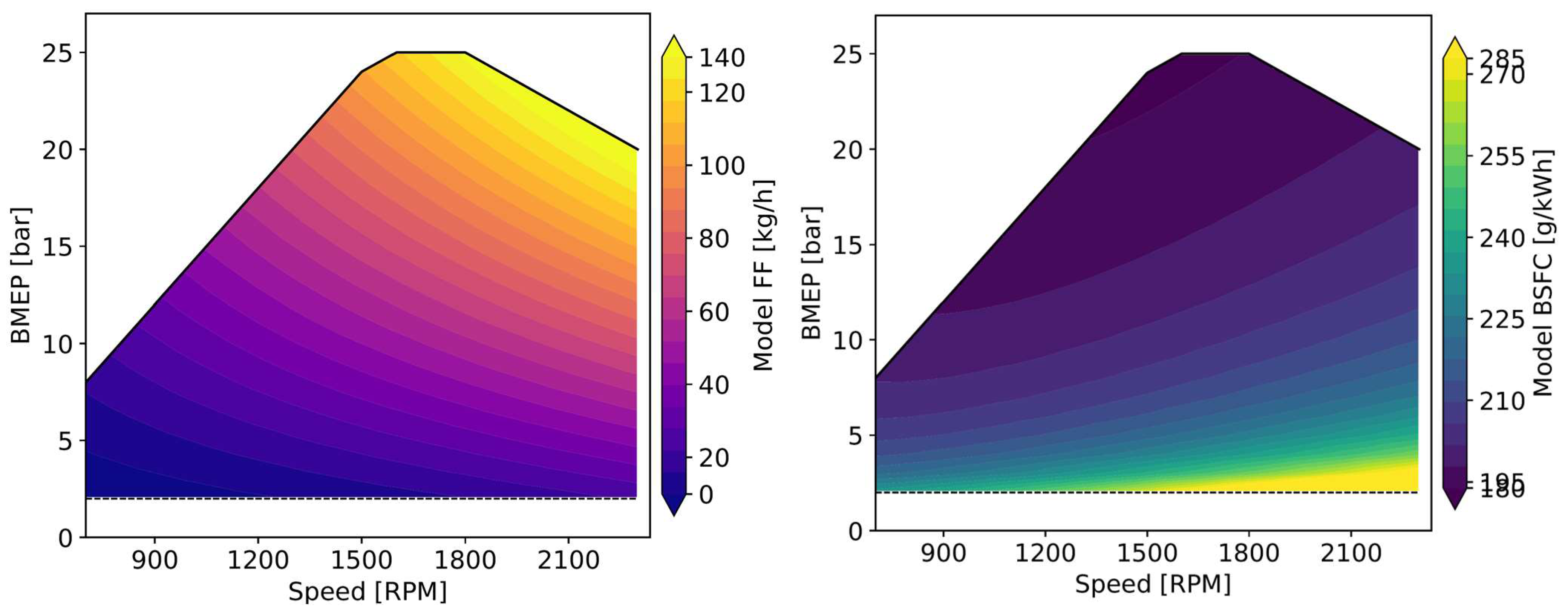
Rapid concept-phase evaluation of hybrid architectures requires simplified engine representations that are both parametric and sufficiently faithful to measured data. Anselma [4] identified this as a standing challenge in HEV powertrain design, demonstrating that dynamic-programming-based screening tools can evaluate candidate architectures with near-optimal accuracy at low computational cost, provided that engine map fidelity is maintained. García et al. [5] illustrated the practical consequence; in a study screening parallel hybrid truck architectures against 2025 European CO₂ targets, the quality of the engine BSFC map used in the simulation determined whether candidate architectures met the regulatory threshold. Both studies confirm the need for a systematic method for generating credible engine maps from readily available inputs alone.

The method of this paper addresses this need directly. Given only a required power output and an application class, it synthesizes an engine model including a torque curve and a BSFC map as a function of speed and load, representative of what a modern production engine could be expected to deliver. The result is a fast-running model suitable for use in comparative studies of diesel and diesel-electric hybrid powertrains, where the goal is to select the most favourable hybrid architecture or to quantify the fuel efficiency benefit of hybridization against a non-hybrid baseline. Conventional engine simulation requires detailed proprietary data that are rarely available at the concept phase and involves significantly greater setup effort and computational cost. The synthesis method of this paper is offered as a practical alternative for concept-phase hybrid powertrain design, where speed and accessibility of the engine model matter more than the fidelity and flexibility of a full simulation.

The relationship between engine displacement, rated speed and peak performance has been studied for spark-ignition engines by Chon and Heywood [6], who compiled 1999 model-year US production engine data and developed correlations between maximum torque, power, and BMEP against geometric parameters including displacement and bore-to-stroke ratio. Engine design features such as valve count per cylinder, supercharging, turbocharging, and compression ratio and general technological improvement over time accounted for significant variations in power density. Heywood and Welling [7] extended this analysis using US, European, and Japanese market databases from 2000 to 2008, demonstrating that established scaling laws give good correlations across the full range of automotive engine sizes when performance is normalized by maximum mean piston speed and total piston area. The mean-piston-speed formulation captures a fundamental mechanical constraint: gas-exchange resistance imposes an upper limit of approximately 12–15 m/s on mean piston speed regardless of engine size [6], and since mean piston speed is proportional to stroke and rated RPM, and breathing and thermodynamic considerations narrow the practical range of bore–stroke ratio, this limit tightly constrains the rated-speed range available for a given displacement. The correlation between stroke and cylinder displacement makes it possible to use cylinder displacement as a surrogate for stroke as a modelling input.

Suijs and Verhelst [8] applied this framing to large-bore spark-ignition gas engines for stationary combined heat and power applications. Menon and Cadou [9] demonstrated that peak power and torque in miniature two-stroke engines also follow power-law scaling with displacement, confirming that the mean-piston-speed limitation operates consistently across a very wide range of engine sizes. The diesel combustion scaling literature provides additional support for family stratification: Stager and Reitz [10], Staples et al. [11], and Lee et al. [12] show that real engineering constraints—bore limits, injector geometry, and compression ratio—cause systematic, class-dependent departures from idealized geometric scaling.

Despite this body of work, no published study has systematically developed engine synthesis correlations for the four application classes most relevant to diesel-electric powertrain hybrid screening: Family 1, automotive/light commercial; Family 2, medium and heavy-duty truck; Family 3, off-highway agricultural and construction; and Family 4, military. Heywood and Welling [7] drew exclusively from automotive market databases and presented very little diesel data. Suijs and Verhelst [8] covered large-bore stationary spark-ignition engines. The off-highway and military classes operate under different duty cycles and are subject to different BMEP and rated-speed design conventions. They have not previously been treated as distinct families in a published engine synthesis or efficiency scaling analysis.

A method is presented for synthesizing a complete diesel engine specification, comprising displacement, cylinder count, rated speed, torque curve, and two-dimensional BSFC map, from a rated power requirement and one of four application classes or families, without measured data. Each family (f = f1, f2, f3 or f4) corresponds to a distinct emissions certification framework: Family 1 engines are certified under the Euro 6/EPA Tier 2–3 light-duty vehicle regulations; Family 2 under the EPA (US Environmental Protection Agency) Heavy-Duty Highway and Euro VI heavy truck regulations; Family 3 under the EPA Non-Road Compression-Ignition (NRCI) and EU Non-Road Mobile Machinery (NRMM) regulations; and Family 4 engines are largely outside civil certification frameworks entirely, being subject instead to military procurement specifications, reflecting the different duty-cycle and reliability requirements of tactical vehicle applications.

The model supports comparison of alternative cylinder counts, for example, selecting between a 4- and a 6-cylinder engine for a given power requirement. This is most relevant when the engine will be purchased from a supplier rather than manufactured in-house, as each candidate involves some engineering work to assess packaging, weight, and integration, and reducing the number of candidates to investigate has practical value. The method is not intended to guide the redesign of an existing engine block.

It is not possible or desirable for the purpose of trade studies to match all available engines, since they differ from one another, but only to ensure that the resulting synthesized engine characteristics fall credibly among the performance capabilities of commercially available engines today. The method supports continuous scaling and is applicable to any concept-phase electrification study where the engines are to be defined rather than matched to an existing unit. As an example application, when a new vehicle platform is being planned, the method can synthesize a set of performance targets for the exact engine required, with the reasonable expectation that current manufacturing technology can deliver an engine to meet those targets. The complete calculation chain can be replicated in a standard Excel spreadsheet and is very suitable for incorporation into larger optimization programmes.

2. Materials and Methods

The synthesis chain described in the Introduction requires empirical correlations for each of its six steps. The steps are developed in this section with reference to a compiled dataset of production diesel engine specifications. Step 6, the generation of the BSFC map from the synthesized specification, uses an enhanced version of the ISFC-FMEP (indicated specific fuel consumption) correction method described in [13], with family-specific class constants derived in Section 2.14 and Section 3.2. The dataset and its preparation are described first, followed by each modelling step in sequence.

2.1. Engine Specification Dataset

Performance specifications for production diesel engines were collected to support the development and validation of the synthesis correlations presented in this paper. Parameters were sought that are both routinely published by engine manufacturers and informative for predicting engine geometry and performance from a power requirement. The parameters sought were: rated power output and the engine speed at which it is achieved; peak torque and the engine speed at which it is achieved; engine displacement; bore and stroke; idle speed; and number of cylinders. Where available, minimum BSFC and the speed and load at which it occurs were also recorded, though these proved to be sparsely populated. Twenty-three usable diesel BSFC maps were identified from published literature and used for correlation. The larger dataset of engine metadata and the smaller dataset of BSFC maps are both publicly available on Zenodo [14].

Four families of diesel engines were defined according to application, reflecting the principal markets in which compression-ignition powertrains are specified for new vehicle designs, and also delineated by regulatory emissions class: Family 1, passenger car and light commercial automotive engines; Family 2, heavy-duty highway truck engines; Family 3, off-highway agricultural and construction equipment engines; and Family 4, military tactical wheeled vehicle engines. This classification broadly follows the application categories used in emissions certification, though it is defined here by end-use rather than by regulatory framework.

Engine metadata were obtained from three primary sources. For Families 1 and 4, manufacturer technical documentation and published OEM (Original Equipment Manufacturer) datasheets were used. For Family 2, the US EPA heavy-duty highway engine certification database (model years 2015–present) [15] provided a comprehensive record of current production engines. For Family 3, the EPA NRCI certification database (model years 2011–present) [16] was supplemented with published OEM brochures from John Deere Power Systems [17] and Deutz AG [18]. The raw compiled dataset, prior to any filtering, is available at [14].

The compiled dataset was refined to produce a working list of engines representative of what might reasonably be specified for a new vehicle architecture. Engines were excluded on several grounds. Naturally aspirated (NA) and indirect injection (IDI) engines were excluded on the grounds that their thermodynamic performance is significantly below current achievable standards. Within Family 3, engines certified only to US EPA Tier 3 or EU Stage IIIA standards were excluded, with the emissions certification tier serving as a proxy for design vintage in the absence of reliable year data for some records. Engines were excluded where the manufacturer’s peak BMEP across its entire product range fell below 15 bar, since this was found to characterize either very small agricultural engines unsuitable for vehicle powertrain applications, severely de-rated generator set variants, or manufacturers not certified under North American or European emissions frameworks, whose performance specifications were not consistent with current North American and European design practices. Within the retained dataset, records with computed BMEP above 30 bar were examined individually: those attributable to suspect data entries in the certification database were excluded and annotated; records from credible Western manufacturers at BMEP values below 30 bar were retained. Where multiple power ratings were available for a single engine block from a single manufacturer, only the highest-rated variant was retained, on the basis that the synthesis method models engine selection for new vehicle architectures, where de-rated variants are accessible, by applying a scalar de-rating parameter to the maximum-power specification. The refined dataset, with all excluded records annotated with the reason for exclusion, contains 41 Family 1 engines, 23 Family 2 engines, 101 Family 3 engines, and 13 Family 4 engines and is available at [14].

2.2. BMEP at Peak Power

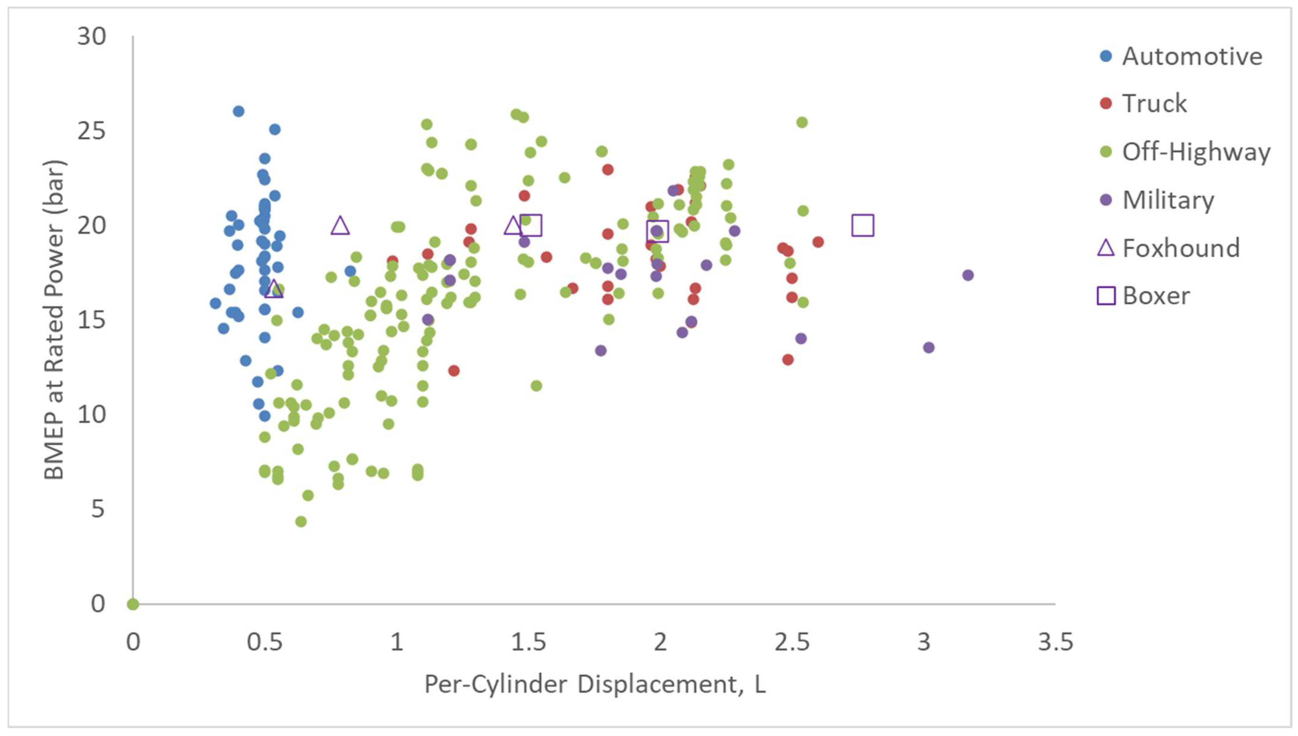
Figure 1 shows rated BMEP (i.e., at the rated power condition) plotted against per-cylinder displacement for all four families. Family 1 has per-cylinder displacements mostly below 0.75 L, presumably to achieve higher rated speeds and better NVH (noise, vibration and harshness). It spans a wide BMEP range of approximately 15–26 bar, reflecting the aggressive downsizing characteristic of modern passenger car diesel development alongside the deployment of cheaper variants for different vehicle types. Family 2 has a relatively tight BMEP band of 12–23 bar, consistent with the convergent regulatory and application requirements of the heavy truck market. Family 3 spans a wider cylinder displacement range, from approximately 0.5 to 2.5 L, with greater scatter in BMEP, reflecting the diversity of agricultural and construction applications. In Family 3, cylinder sizes below 1.25 L contain many examples of very low BMEP, indicating de-rated engine versions for lower-power applications. Family 4 occupies the 1.5–3.5 L range at 12–22 bar. There is no discernible trend in the data, except a preponderance of de-rated engines in the off-highway group, which achieve significantly lower BMEP than others at the same displacement and in the same group.

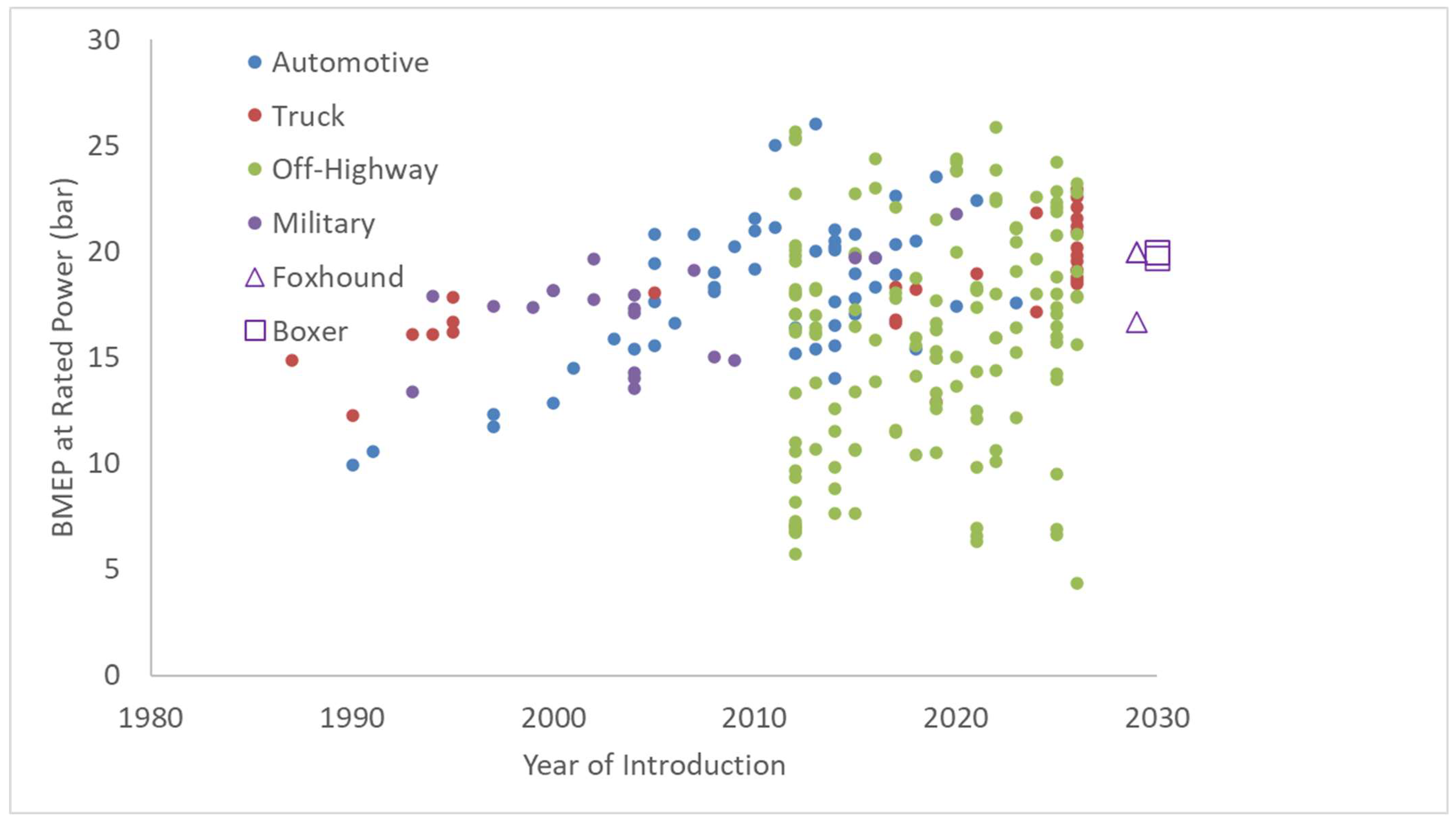
Figure 2 also shows BMEP at rated power but plotted against year of engine introduction. No systematic trend is visible after about 2010, after the Tier 4 Interim (2012–13) and earlier cohorts. Many commercial diesel engines are offered in a range of power outputs based on the same engine block, for reasons of complexity, package and manufacturing investment, and this is seen particularly in the range of the off-highway family. In the years 2025–2026 the values cluster around 18–22 bar if the downrated off-highway outliers are excluded.

An engine for a new powertrain architecture would not be specified in a de-rated form at low BMEP, so a common value of 20 bar at rated speed is assumed as a universally achievable value for modern diesel engines, for the purpose of engine synthesis, across all families.

2.3. BMEP at Peak Torque

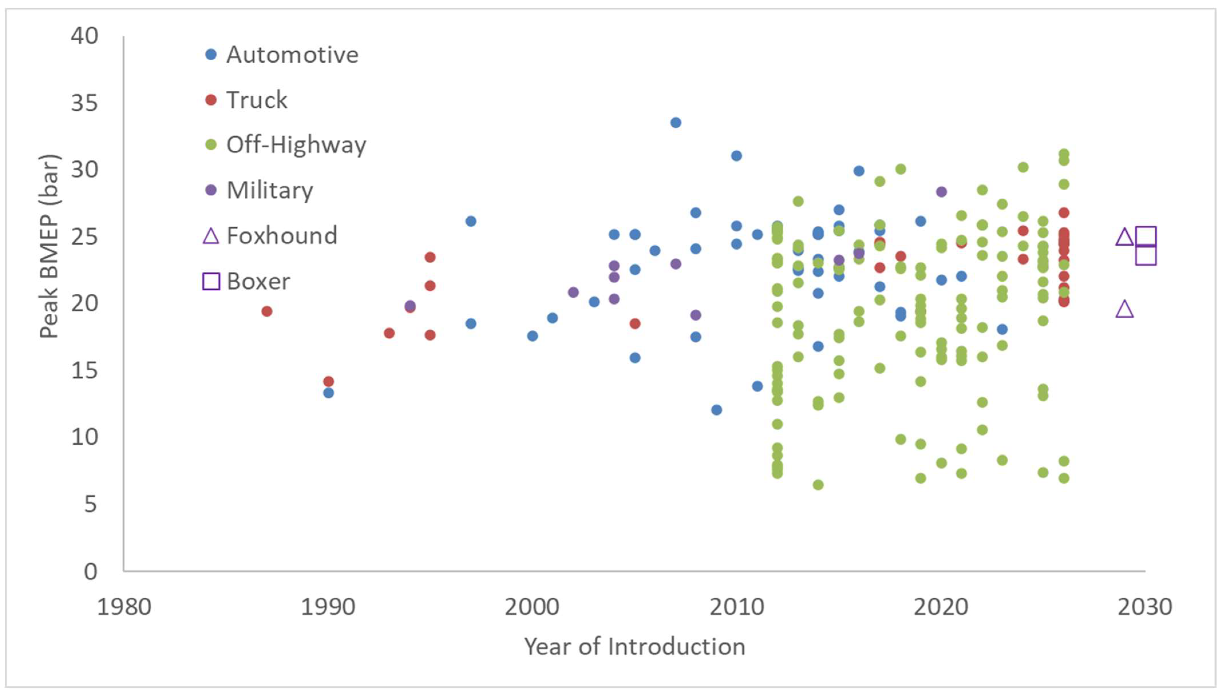
Figure 3 plots BMEP at peak torque against year of introduction for all four engine families. From 2020 to 2026, excluding the obviously downrated engines in the off-highway family, peak BMEP is in the range 20–30 bar. A common maximum BMEP of 25 bar is adopted as an achievable value for all engine families for the purpose of engine synthesis.

2.4. Number of Cylinders

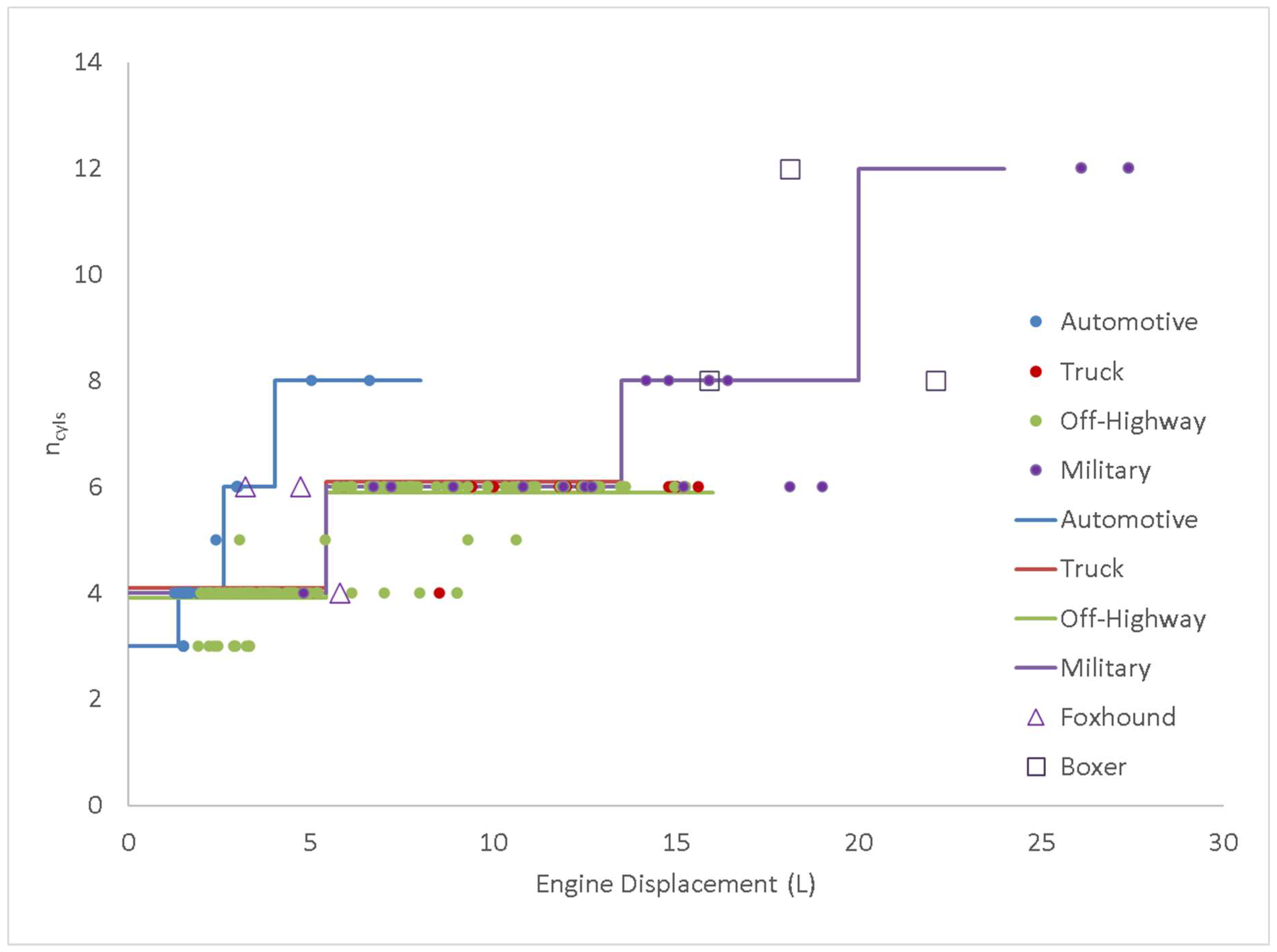
The synthesis model requires a method to assign cylinder count according to its inputs, but in many cases, more than one valid choice exists. For each family, the displacement range occupied by each cylinder count was examined, and the mid-point of the gap between adjacent populations was taken as the threshold. Where no clean gap existed—that is, where the displacement ranges of adjacent cylinder counts overlapped—the mid-point of the overlap zone was used instead. Five-cylinder engines (one entry in Family 1, four entries in Family 3, all Scania) were excluded as a niche historical configuration not relevant to current design practice. Six large-bore four-cylinder entries in Family 3 (Liebherr specialist configurations and the Deutz TCD 9.0) were excluded as architectural outliers, with no mainstream design precedent above 5.5 L. Figure 4 plots cylinder count against total displacement for all four engine families. The cylinder count thresholds derived from this analysis are summarized in

Table 1. Cylinder count selection thresholds adopted in the model. Displacement values mark the boundary at which the tool transitions to a higher cylinder count for each engine family.

Family 4 (Military)	Families 2 & 3 (Truck/Off-Highway)	Family 1 (Automotive)	Transition
—	—	1.37 L	3 → 4 cyl
5.40 L	5.40 L	2.60 L	4 → 6 cyl
13.5 L	16.0 L	4.00 L	6 → 8 cyl
20.0 L	20.0 L	—	8 → 12 cyl

.

2.5. Engine Speed at Rated Power and at Peak Torque

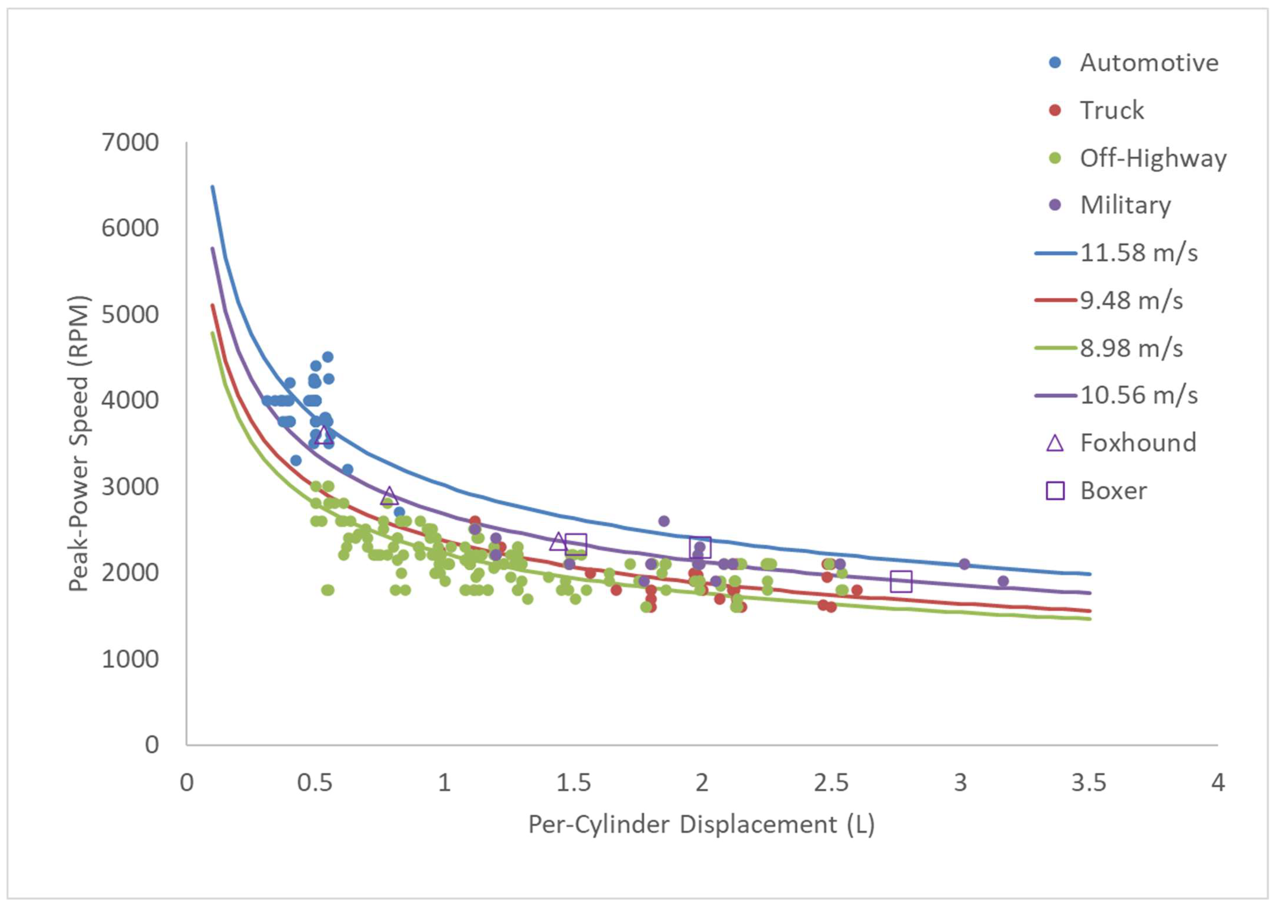
Figure 5 shows rated speed (RPM) versus cylinder displacement for the four engine families. Rated speed is the speed at which the rated power of the engine is quoted, and in practice the maximum speed of the engine is a little higher than the rated speed. All families display higher rated speed for smaller cylinders, due partly to piston speed durability constraints and partly to gas dynamics. Automotive engines are designed for higher operating speeds, in order to achieve higher power density and respond to rapid changes in road speed, and tend to deploy smaller cylinders as a result. Truck engines are optimized for longevity and efficient operation over a narrow band of speed, with narrow-spaced gears and frequent shifts, tolerating a smaller useful speed band, so larger cylinders are practical. Military engines have lower operating hours over their lifetime and need higher power density. Off-highway engines operate at lower speeds to prioritize longevity and efficiency.

Each family’s data follows a hyperbolic relationship between rated speed and per-cylinder displacement. This arises from a durable mean-piston-speed ceiling: since mean piston speed is S_p = 2LN_s, and stroke L is determined by cylinder displacement and bore-to-stroke ratio κ through Equation (10), defined in Section 2.14, rated speed at the ceiling is directly expressed as a function of per-cylinder displacement. In the expression S_p = 2LN_s, N_s is engine speed in rev/s; note that, elsewhere in this paper, engine speed is expressed in RPM, with the factor 1200 in Equations (4), (12) and (14) absorbing the conversion.

At rated speed:

$$N_{rated}=30· S_{p,max} ·{({\pi \kappa }^2/\left(4· D_{cyl}\times {10}^{-3}\right)) }^{1/3},$$

(1)

$$D_{cyl}={\displaystyle \frac{V_d}{N_{cyl}}},$$

(2)

where N_rated is the rated speed in RPM; D_cyl is the per-cylinder displacement in litres; κ is the family-mean bore-to-stroke ratio; and S_p,max (m/s) is the maximum mean piston speed for the engine family. The bore-to-stroke ratio κ is the family constant adopted in

Table 2. Maximum mean piston speed S_p,max and bore-to-stroke ratio κ for each engine family. S_p,max is derived by fitting N_rated vs. D_cyl data for each family.

Engine Family	κ	Sp,max (m/s)
Automotive	0.909	11.58
Truck	0.857	9.48
Off-Highway	0.845	8.98
Military	0.877	10.56

. S_p,max is determined for each family by fitting the constant-S_p hyperbola to the N_rated versus D_cyl scatter by least-squares optimization of S_p. Figure 5 shows the resulting hyperbolae. The four S_p,max values are listed in Table 2, together with the family κ values from Section 2.7 on which the hyperbola geometry depends. The resulting S_p,max values are consistent with published guidance on mean-piston-speed durability limits for four-stroke diesel engines ([19], Ch. 2), and they appear as hyperbolic lines with one value for each engine family (Table 2) in Figure 5.

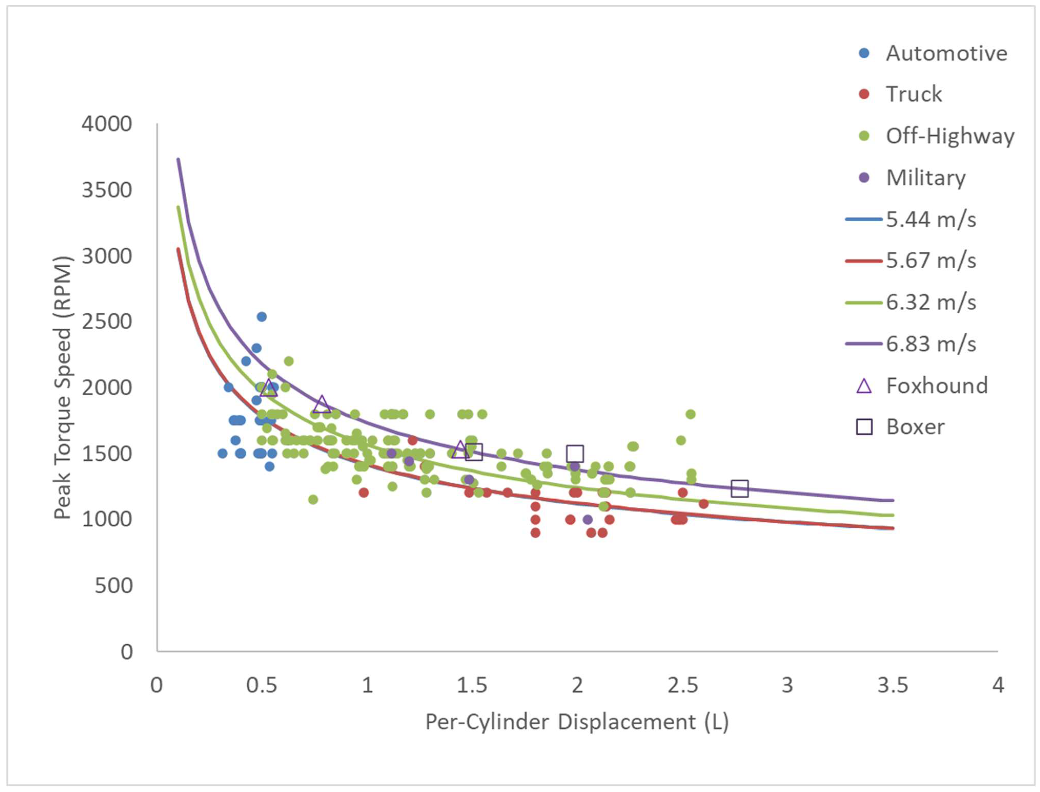
The same procedure is followed for engine speed at peak torque.

Figure 6 plots the speed at peak torque against displacement per cylinder. The fitted relationship is given in Equation (3):

$$N_{pktq}= {30· S}_{p,pktq}·{({\pi \kappa }^2/\left(4· D_{cyl}\times {10}^{-3}\right)) }^{1/3},$$

(3)

where N_pktq is the speed at peak torque in RPM; D_cyl is the per-cylinder displacement in litres; κ is the family-mean bore-to-stroke ratio; and S_p,pktq (m/s) is the mean piston speed at peak-torque speed. The values of S_p,pktq are shown in

Table 3. Mean piston speed at peak torque adopted for each engine family.

Engine Family f	Sp_pktq (m/s)
Automotive	5.44
Truck	5.67
Off-Highway	6.32
Military	6.83

.

S_p,pktq is determined for each family by fitting the constant-S_p hyperbola to the N_pktq-versus-D_cyl scatter by least-squares optimization, as with S_p,max.

2.6. Displacement–Power Relationship and Reverse Lookup

A relationship between engine displacement and maximum power may be derived by taking engine family and displacement as inputs and then deriving a continuous relationship, resulting in maximum power as output.

Combining the results in Section 2.2 and Section 2.3 with the standard four-stroke power relation [19] gives rated power as an explicit function of displacement and engine family:

$$P_{rated}\left(V_d, f\right)={\displaystyle \frac{{BMEP}_r·V_d·N_{rated}}{1200}},$$

(4)

where BMEP_r is the family-mean rated BMEP (taken as 20 bar from the survey in Section 2.1), and f denotes the engine family (f1–f4); V_d is total displacement in litres; N_rated is the rated speed in RPM from Equation (1), evaluated at D_cyl = V_d/n_cyl from Table 1; and the constant 1200 absorbs the four-stroke factor of 2 and the RPM-to-rev/s, bar-to-kPa, and litres-to-m³ conversions simultaneously. 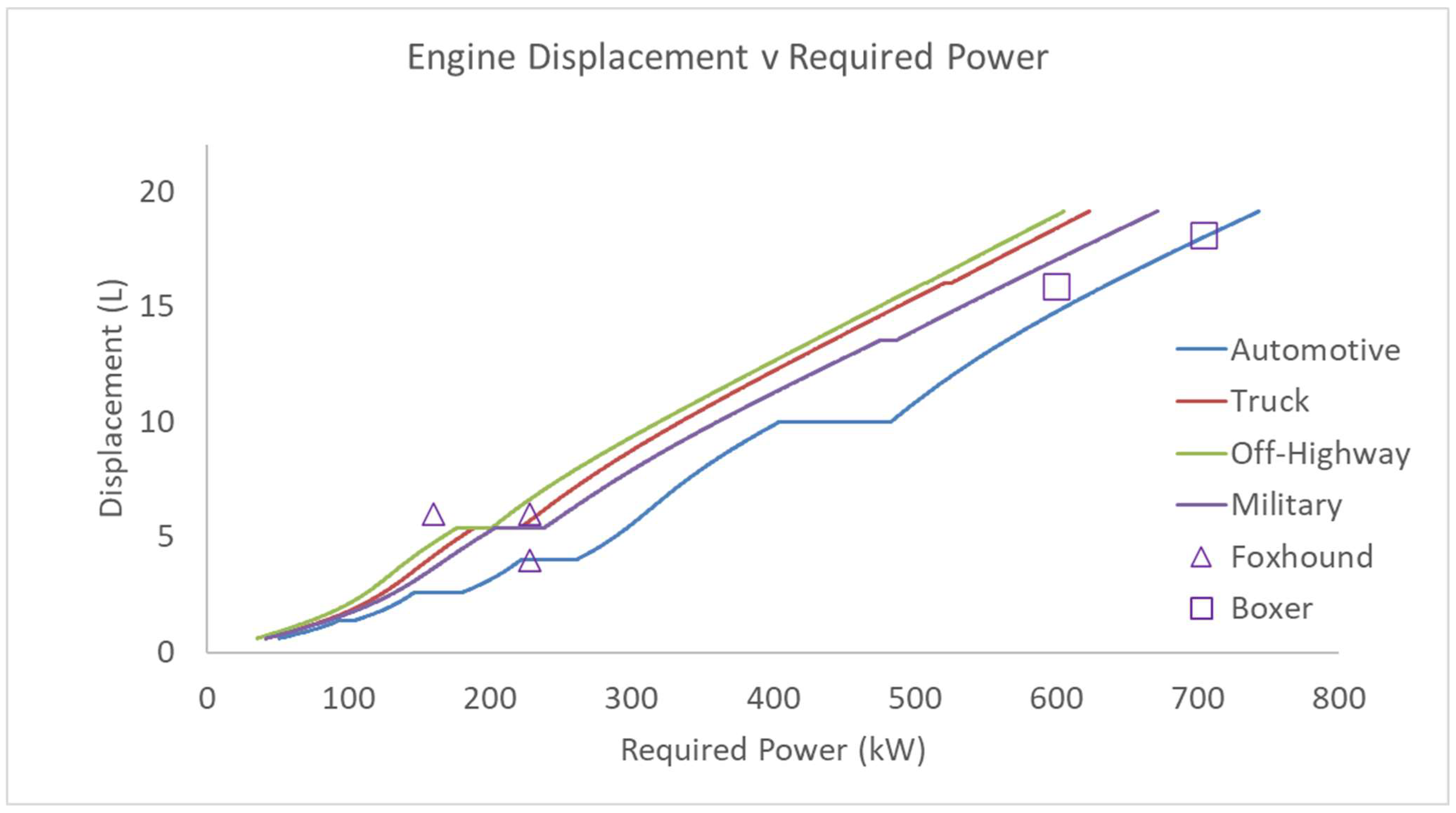Because N_rated is a stepped function of V_d, Equation (4) is non-monotonic in V_d: at each cylinder-count increase the jump in rated speed raises specific power, creating the choice points illustrated in Figure 7.

Table 4. Example calculation steps relating displacement (L) to rated power (kW) for family f3.

Engine Family	Displ (L)	Cylinders	Cylinder Displ (L)	Rated BMEP (bar)	Rated Speed (RPM)	Power (kW)
Off-Highway	3	4	0.75	20	2438	122
Off-Highway	5	4	1.25	20	1995	166
Off-Highway	6	6	1	20	2138	214
Off-Highway	15	6	2.5	20	1901	475
Off-Highway	17	8	2.12	20	1903	539
Off-Highway	19	8	2.38	20	1901	602
Off-Highway	21	12	1.75	20	1913	671

shows the results of this calculation path for selected values.

Figure 7 shows that the relationship between required power and engine displacement is non-monotonic at cylinder-count transitions. This arises because the algorithms automatically select 3, 4, 6, 8 or 12 cylinders according to displacement, but the change to a larger number of cylinders automatically improves specific power (kW/L) by allowing a higher rated speed. The engineer specifying a powertrain architecture is therefore faced with a choice at some desired power levels. For example, when specifying an engine for an off-highway application at 180 kW, the designer may choose a 6-cylinder engine of displacement 4.4 L or a 4-cylinder engine of 5.5 L; both deliver 180 kW, though at rated speeds of 2473 RPM and 1958 RPM respectively. While a lower cylinder count generally offers lower weight and cost, several other factors might in practice drive this choice towards the higher cylinder count, including NVH (noise, vibration and harshness), a preference for higher rated speeds, availability, and package.

To avoid repeated numerical inversion of Equation (4) in optimization scenarios, the power–displacement relationship can be precomputed as a lookup table P_lookup. For each cylinder count n_cyl ∈ {3, 4, 6, 8, 12} and total displacement V_d sampled at uniform step ΔV_d over [V_d,min, V_d,max], the rated power is

$$P\left(V_d, n_{cyl}, f\right)={\displaystyle \frac{{BMEP}_r·V_d·N_{rated}\left(\frac{V_d}{n_{cyl}}, f\right)}{1200}},$$

(5)

where P(V_d, n_cyl, f) is the tabulated rated power in kW; BMEP_r is the family-mean rated BMEP (set to 20 bar, Section 2.1); and N_rated(V_d/n_cyl, f) is the rated speed from Equation (1) evaluated at per-cylinder displacement V_d/n_cyl. Each column of P is monotonically increasing in V_d, so reverse lookup within any column reduces to linear interpolation between two bracketing rows.

Given a required power P_ref and engine family f, the reverse lookup proceeds as follows.

For each n_cyl, use table P_lookup to establish the displacement V_d required to achieve the required power P_ref for this value of n_cyl and the selected engine family. If the resulting V_d falls within the valid range for the selected engine family, then this combination of V_d and n_cyl is valid. Where more than one combination is valid, select the higher-n_cyl alternative for a smaller, faster engine, or the lower-n_cyl sub-column for a larger, slower engine with more peak torque. If no sub-column qualifies, P_ref is outside the achievable range for this family. Flag an error.

A grid step of ΔV_d = 0.05 L is sufficient; since each column is nearly linear in V_d over short intervals, the interpolation error is below 1% across the full displacement range. The precomputed table for each family is the data underlying Figure 7, so the table construction and the figure are the same computation.

2.7. Idle Speed

Current automotive diesel practice places idle speed in the range 650–800 rpm, with most modern passenger car engines settled at approximately 700–750 rpm. Larger-displacement heavy-duty, off-highway, and military engines typically idle somewhat lower, in the 600–700 rpm range, owing to higher rotational inertia and a lower friction-to-displacement ratio at low speed. Accordingly, an idle speed of 750 rpm is assigned to Family 1 (automotive) engines, and 650 rpm to Families 2, 3, and 4 (truck, off-highway, and military).

2.8. Maximum Speed

The rated speed is defined in Section 2.5, and this is taken as the maximum speed for the purpose of engine synthesis.

2.9. Maximum BMEP at Idle Speed

The maximum BMEP that a turbocharged diesel can develop at idle speed is constrained by two limitations. First, turbocharger boost is negligible, so charge density is limited to near-atmospheric conditions. Second, volumetric efficiency at very low crank speed is depressed relative to the mid-speed optimum by gas dynamics tuning optimized for the normal operating range. A naturally aspirated diesel with optimized gas-exchange might sustain 5–7 bar BMEP under these conditions; modern variable-geometry turbochargers (VGTs) can provide a modest increment in boost at idle, raising the ceiling slightly.

The maximum BMEP occurring at the lowest speed represented in each map was extracted for engines whose maps extend to near-idle conditions and whose data are of sufficient quality to support the inference. Maps whose low-speed boundary was produced by numerical scaling or extrapolation rather than measurement were excluded. The results are reported in

Table 5. Maximum BMEP at the lowest speed represented in selected published BSFC maps. Only maps based on measured or independently digitized data are included; scaled or artificially extended maps are excluded.

Engine	Description	V_cyl (cm3)	Min RPM	Max. BMEP (bar)	Source
BMW N57	3.0 L, 6-cyl bi-turbo DI	500	711	8.8	[20]
Mercedes 1.7 L	1.70 L, 4-cyl turbo DI	425	1200	8.5	[21,22]
VW TDI 1.9 L	1.90 L, 4-cyl turbo DI	475	750	5.8	[21,22]
Audi 2.5 L	2.50 L, 5-cyl turbo DI	500	1000	6.9	[21,22]
Mercedes OM611	2.20 L, 4-cyl CRDi turbo DI	550	1250	4.0	[21,22]
Heywood	1.47 L, 4-cyl NA DI	368	1500	6.0	[19]
Heywood	1.99 L, 5-cyl NA IDI	397	1000	6.0	[19]
Heywood	6.54 L, 8-cyl NA DI	818	1000	5.8	[19]

.

The naturally aspirated engines develop 5.8–6.0 bar, consistent with near-ambient charge density and competent breathing without any boost contribution. The turbocharged automotive engines span 4.0–8.8 bar across their lowest tested speeds, reflecting varying degrees of residual boost and differing map coverage limits. The SwRI-measured (Southwest Research Institute) OM611 result of 4.0 bar at 1250 rpm is a lower outlier attributable to the map boundary falling short of the torque curve at that speed rather than to a physical limitation at idle speed.

A uniform value of 8 bar is adopted for synthesis of all engine families. This value lies within the range spanned by the three highest-quality measured maps (8.5 bar for the ORNL-measured (Oak Ridge National Laboratory) Mercedes 1.7 L unit and 8.8 bar for the EPA-measured BMW N57 3.0 L), provides a modest allowance for residual VGT boost above the naturally aspirated ceiling of approximately 6 bar, and represents a conservative upper bound that does not overclaim torque capacity at the curve foot.

2.10. Assembling the Torque Curve

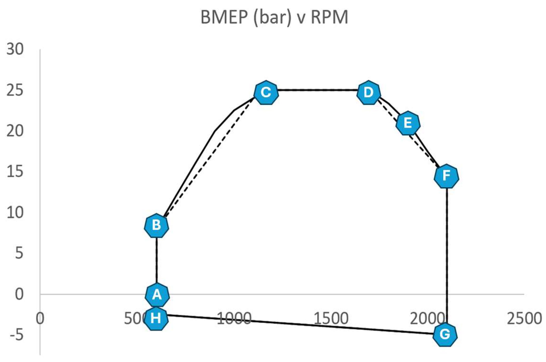
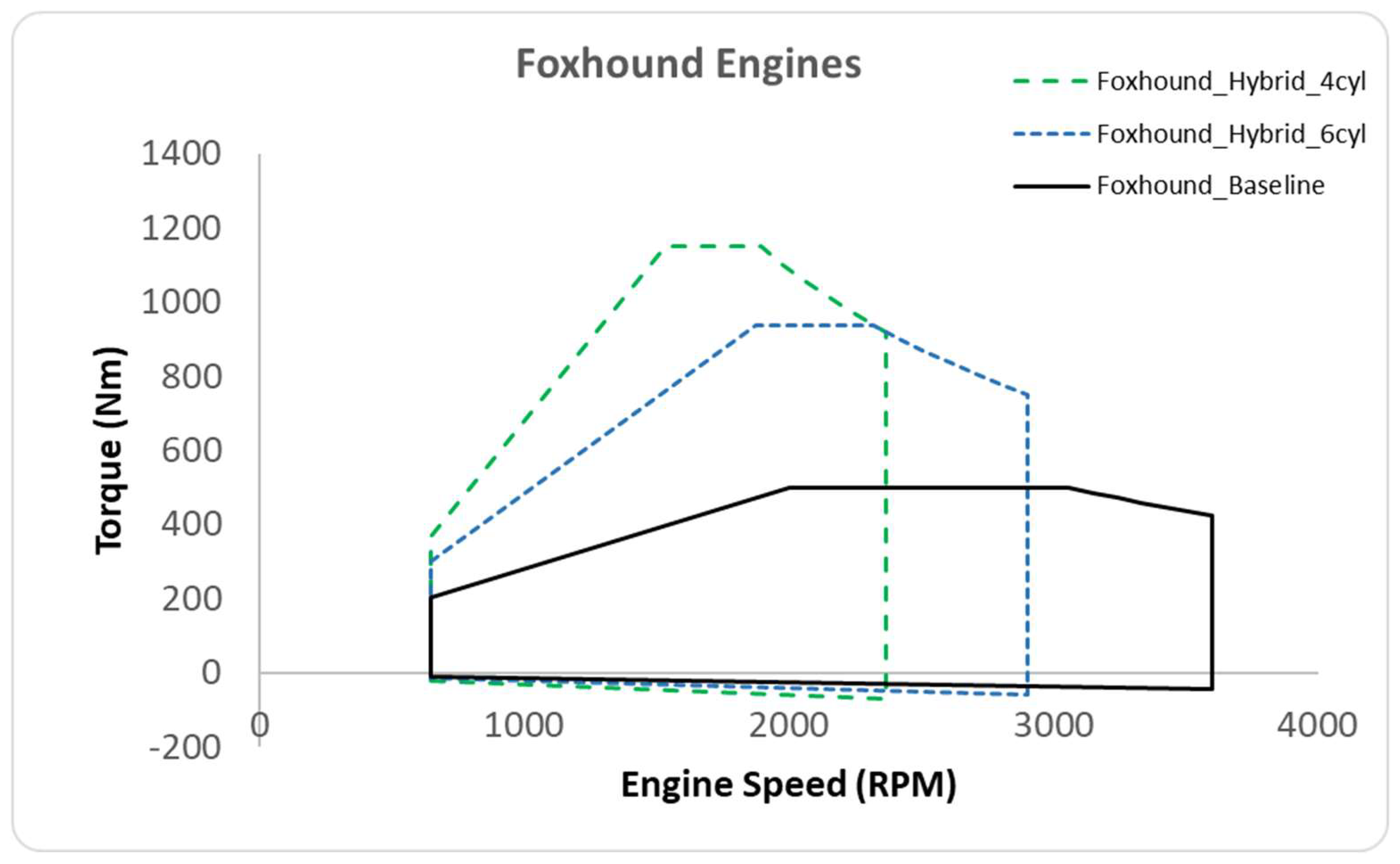
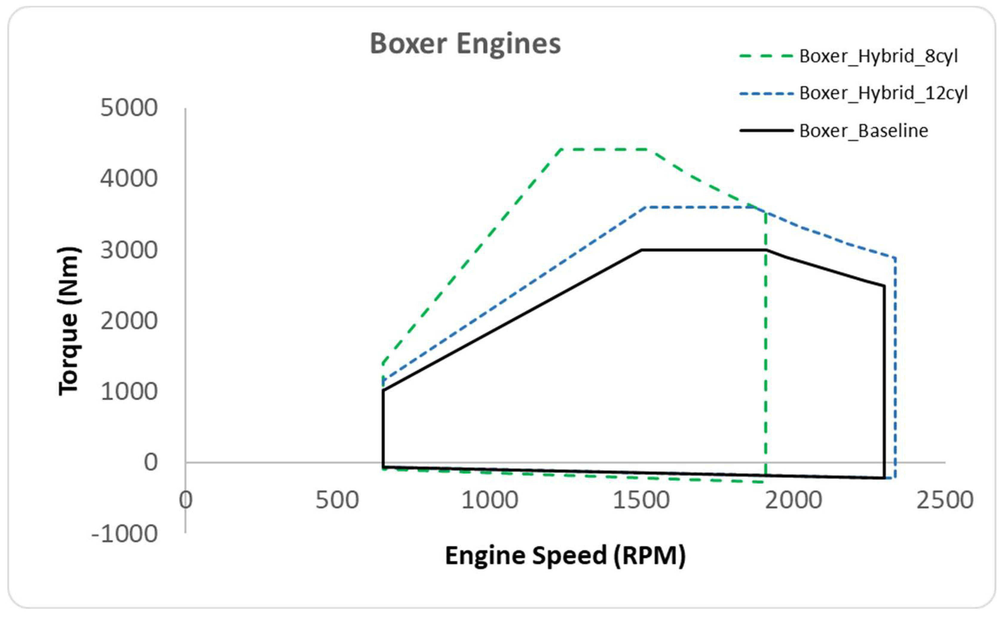
A representative operating envelope for a turbocharged diesel engine is shown in Figure 8 as a solid line. As BMEP is proportional to torque, the upper portion from B to F takes the same shape as the torque curve. Point A represents the idle condition, at minimum RPM with zero torque output. B is the highest BMEP achievable at minimum RPM, limited by poor turbocharger boost and sub-optimal breathing dynamics. C is the lowest RPM at which maximum BMEP and maximum torque can be achieved. Turbocharger boost is typically controlled to achieve a constant maximum BMEP for a range of RPM up to point D, after which the BMEP drops off to point E, where rated (maximum) power is obtained. Point F is the maximum BMEP achievable at the maximum RPM. The line from G to H represents the negative “motoring” conditions that occur if the fuel is shut off completely while decelerating or descending a hill. The whole loop, from A to H and back to A, bounds the possible operating conditions of the engine for the purposes of simulation.

For engine synthesis, the simplified shape of the dotted line is adopted, with a straight line between B and C and a curved constant power line from D to F, eliminating point E and making point F the rated power at the rated speed. The speed at point D is defined as that which gives point D the same power as point F.

2.11. Minimum BSFC as a Function of Per-Cylinder Displacement

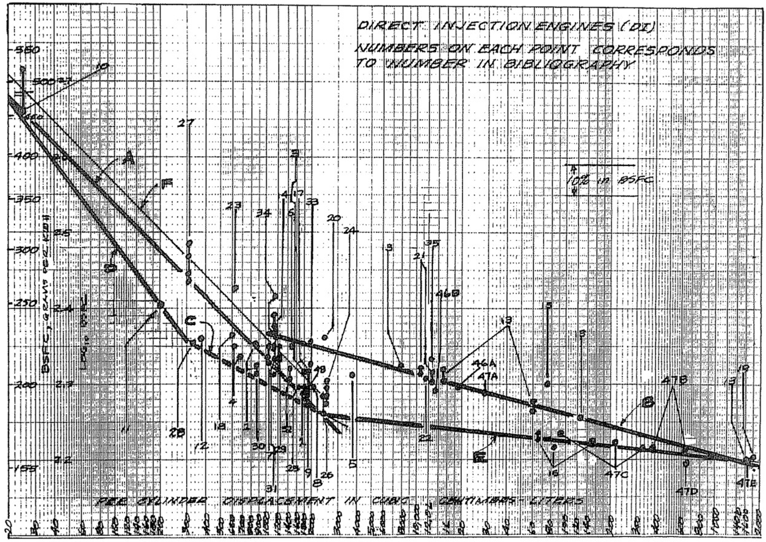
The relationship between minimum BSFC and cylinder displacement extends well beyond the range examined here. Uyehara [23] documented the displacement trend of minimum BSFC across DI (direct injection) diesel engines spanning five orders of magnitude in cylinder size, from a 25.7 cm³ single-cylinder research engine to large slow-speed marine units with per-cylinder displacements on the order of 600–2000 L, as shown in Figure 9. At the upper end of this size range, minimum BSFC values of approximately 155–171 g/kWh are reported, consistent with the thermodynamic floor for diesel combustion. Heywood ([19], Ch. 12) confirms the underlying mechanism: as cylinder volume grows relative to combustion chamber surface area, the fraction of fuel energy rejected to the cylinder walls falls, reducing the thermodynamic floor of fuel consumption.

The functional form of the displacement dependence follows from cylinder geometry. For a cylinder of bore B and stroke L with per-cylinder swept volume V_cyl and a narrow range of practical B/L ratios, the combustion chamber surface area scales as B² while V_cyl scales as B³ at constant bore-to-stroke ratio κ. The surface-to-volume ratio therefore scales as V_cyl^−1/3. Since the fraction of indicated work lost to wall heat transfer is proportional to the surface-to-volume ratio at the time of peak heat release [19], the heat-transfer penalty above the large-cylinder asymptote scales as D_cyl^−1/3. This gives a two-parameter model per family:

$${BSFC}_{min}=r+s · {D_{cyl}}^{-1/3},$$

(6)

where r (g/kWh) is the large-cylinder asymptote representing the thermodynamic floor, and s (g/kWh) is a family-specific scaling coefficient representing the magnitude of the heat-transfer penalty. Both parameters carry direct physical meaning: r is anchored by the large marine engine data from Uyehara [23] and is common to all families at 154 g/kWh; s differs between families, reflecting systematic differences in combustion chamber design, injection technology, and cylinder surface finish.

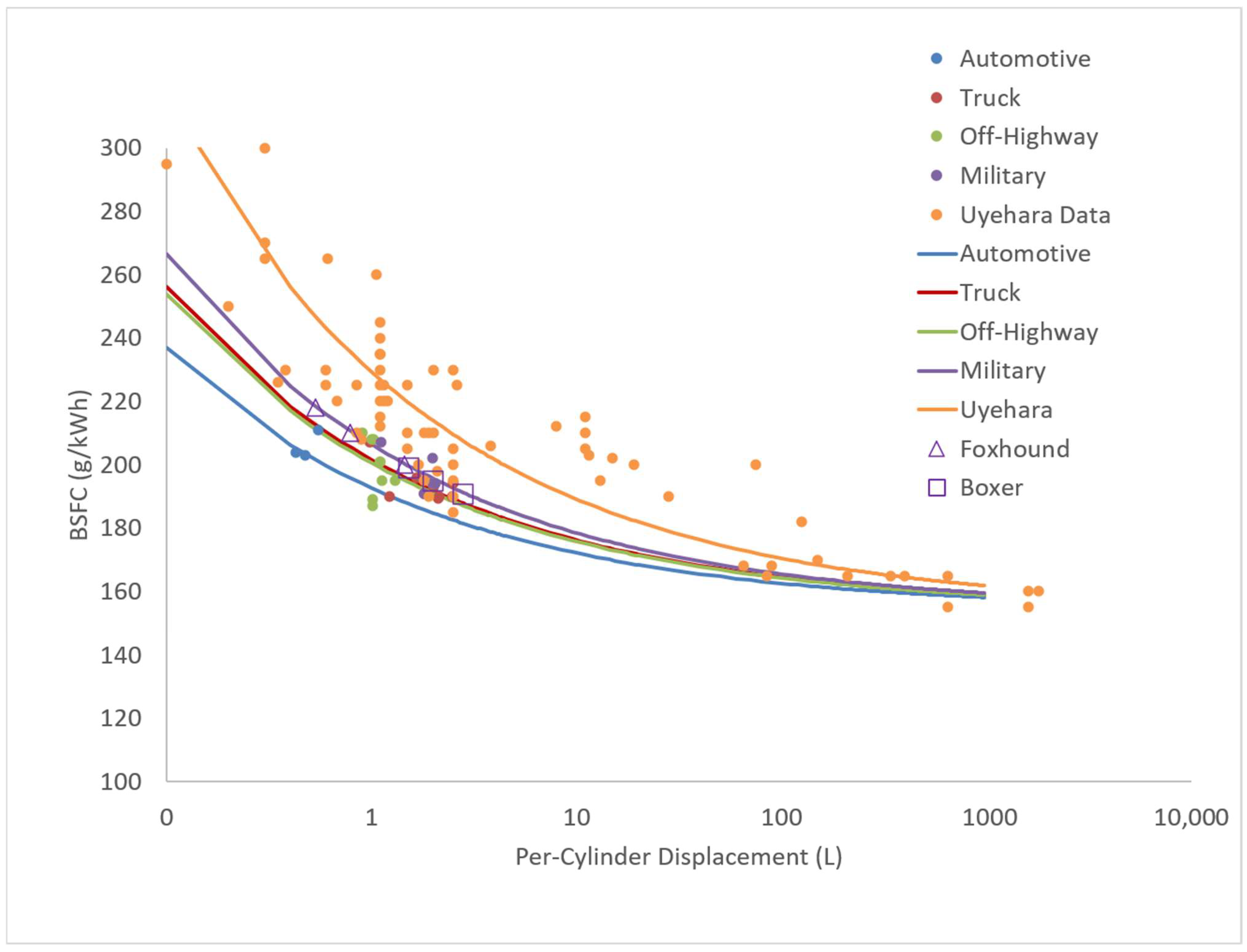
Figure 10 plots minimum BSFC against per-cylinder displacement D_cyl. The dataset for the four modern engine families contains 27 turbocharged DI engines certified to Tier 4 Final or Stage V standard. Additional data points digitized from Uyehara [23], spanning the full range of engine sizes in his Figure 1 (DI engines only), are overlaid to guide the trendlines and establish the large-displacement asymptote. The Uyehara data at small displacement (below approximately 1 L) lie above the modern family curves, consistent with the lower injection pressures and less developed combustion systems pre-1988. At large displacement (above approximately 10 L), the Uyehara points fall below the modern family curves, reflecting the absence of emissions-related fuel consumption penalties in unconstrained marine and industrial engines and the DI combustion systems used for large cylinders long before they were developed for road vehicles.

The exponent of 1/3 is fixed on physical grounds for all families. The coefficient s is fitted to each family’s data by minimizing the sum of squared residuals. The fitted coefficients are given in

Table 6. Coefficients r and s for Equation (6). The exponent α = 1/3 is common to all families. r is the large-cylinder BSFC asymptote; s is the displacement-dependent scaling coefficient. The Uyehara row is shown for reference and is not used in the synthesis chain.

Engine Family	r (g/kWh)	s (g/kWh)	Exponent α
Automotive	154	38	1/3
Truck	154	47	1/3
Off-Highway	154	46	1/3
Military	154	52	1/3
Uyehara Data	154	75	1/3

. The Uyehara dataset is fitted separately for reference; its higher value of s relative to the modern families reflects both the older injection technology at small bore and the absence of Tier 4/Stage V efficiency penalties at large bore, which together steepen the displacement dependence of BSFC across the full size range of the survey. Equation (6), with the coefficients in Table 6, is adopted as the default minimum-BSFC estimate for a synthesized engine when no datasheet value is available; a known published value may be substituted directly, as described in Section 2.17.

2.12. BSFC Map Generation

The preceding steps of the synthesis chain produce rated power, displacement, cylinder count, rated speed, and minimum BSFC for a synthesized engine. The final step generates a two-dimensional fuel consumption surface over the full operating envelope of engine speed and load. Fuel flow rate is adopted as the primary model output rather than brake-specific fuel consumption (BSFC), because BSFC is ill-defined at zero torque. BSFC can be calculated as a secondary quantity wherever power is non-zero.

2.13. Net Mean Effective Pressure Convention

Brake mean effective pressure is related to indicated and friction mean effective pressure by

$$BMEP={IMEP}_{net}-FMEP,$$

(7)

where IMEP_net is the net indicated mean effective pressure, computed over the complete four-stroke cycle including the gas-exchange strokes. Pumping work is therefore absorbed into IMEP_net and requires no separate PMEP term. FMEP consequently represents all mechanical dissipation not captured by the net indicated work.

2.14. Friction Model

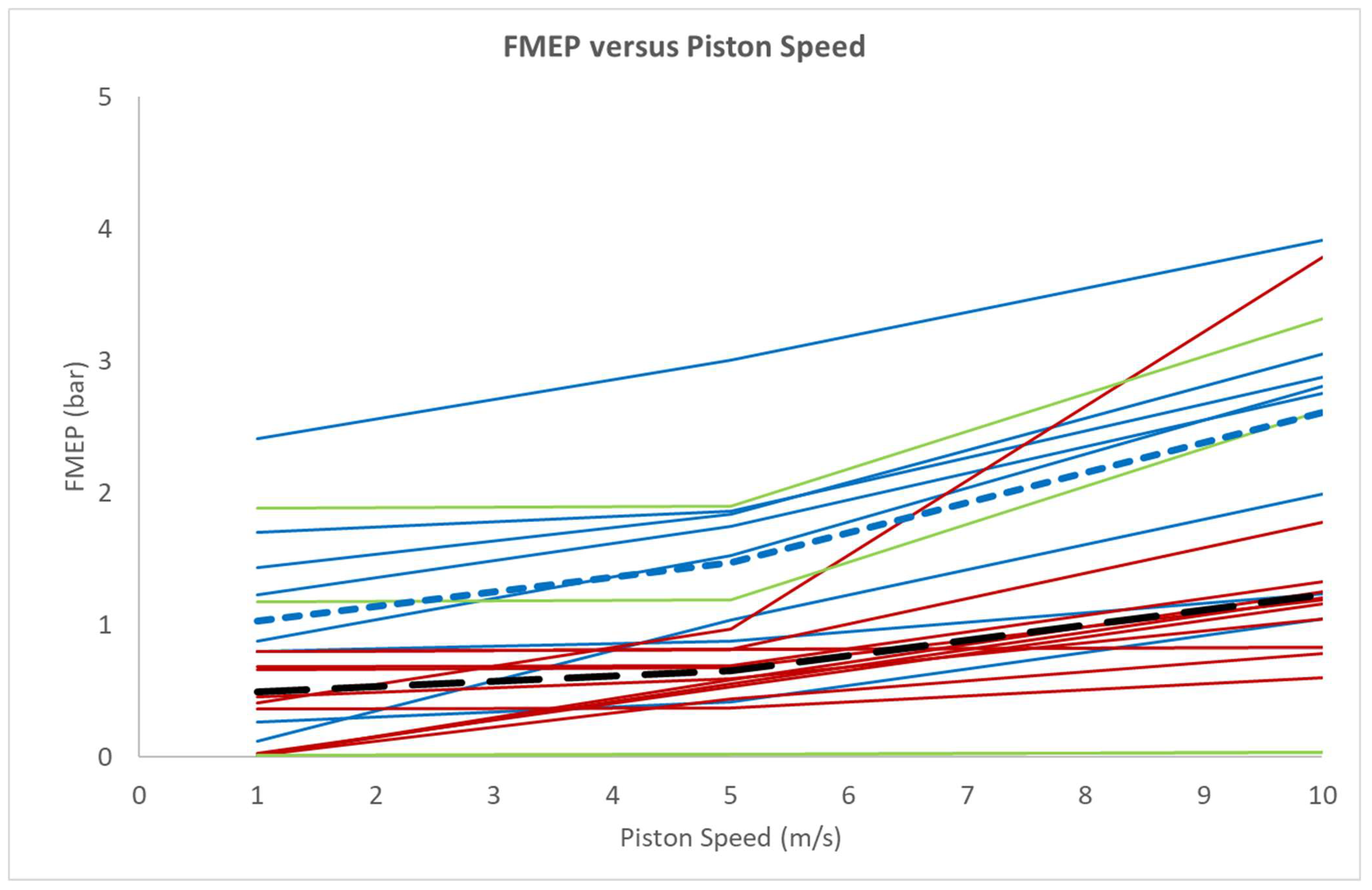
FMEP is modelled as a quadratic function of mean piston speed S_p, following Chen and Flynn [24]:

$$FMEP\left(S_p\right) = C_0 + C_1·S_p + C_2·S_p^2,$$

(8)

where mean piston speed is

$$S_p=2·L·N_s,$$

(9)

where N_s is engine speed in rev/s. Note that engine speed is expressed in RPM elsewhere in this paper; Equations (4), (12) and (14) use N in RPM, with the factor 1200 absorbing the rev/s-to-RPM conversion.

The original Chen–Flynn correlation [24] also includes a peak-cylinder-pressure term B·P_max, which is omitted here for simplicity. The accuracy of fit is sufficient for this purpose without it; calibration against net BSFC map data absorbs the load-averaged effect of pressure-dependent ring friction into C₀. Stroke L is not a direct synthesis output; it is recovered from per-cylinder displacement and a family-typical bore-to-stroke ratio κ = B/L:

$$L = {\left({\displaystyle \frac{4·V_{d,cyl}}{\pi ·k^2}}\right)}^{{\displaystyle \frac{1}{3}}},$$

(10)

where V_d,cyl = V_d/n_cyl is the per-cylinder swept volume.

Mean values of κ for the four engine families from this paper’s dataset are adopted as follows: 0.909 (automotive), 0.857 (truck), 0.845 (off-highway) and 0.877 (military).

2.15. Speed Dependence of Indicated Efficiency

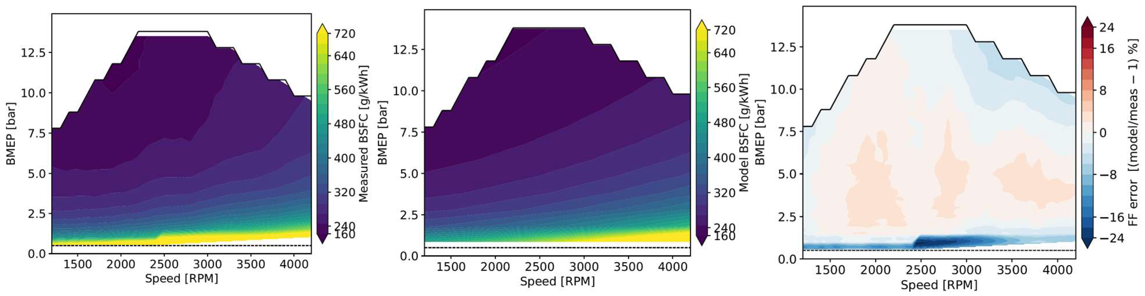
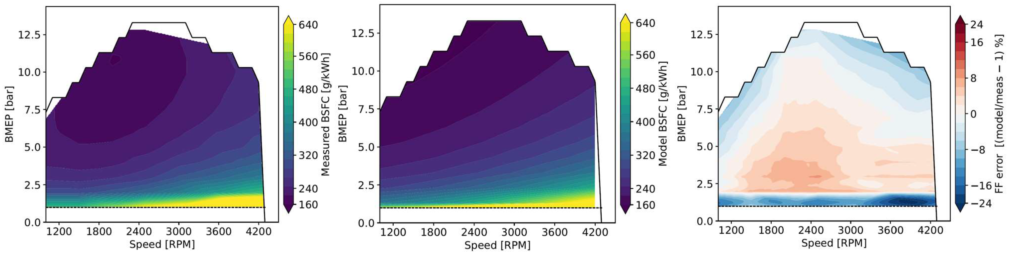
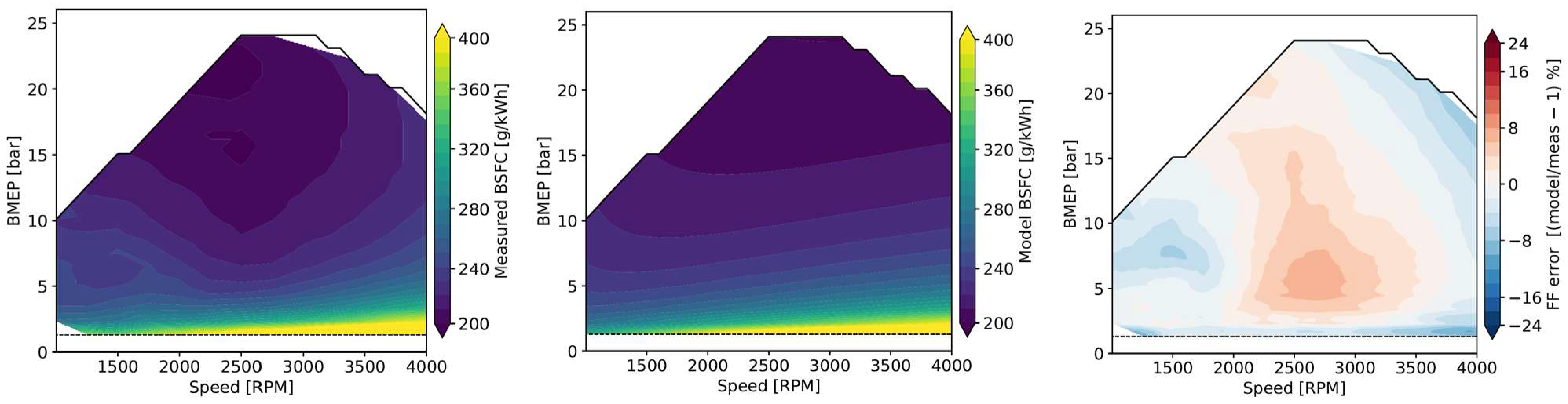
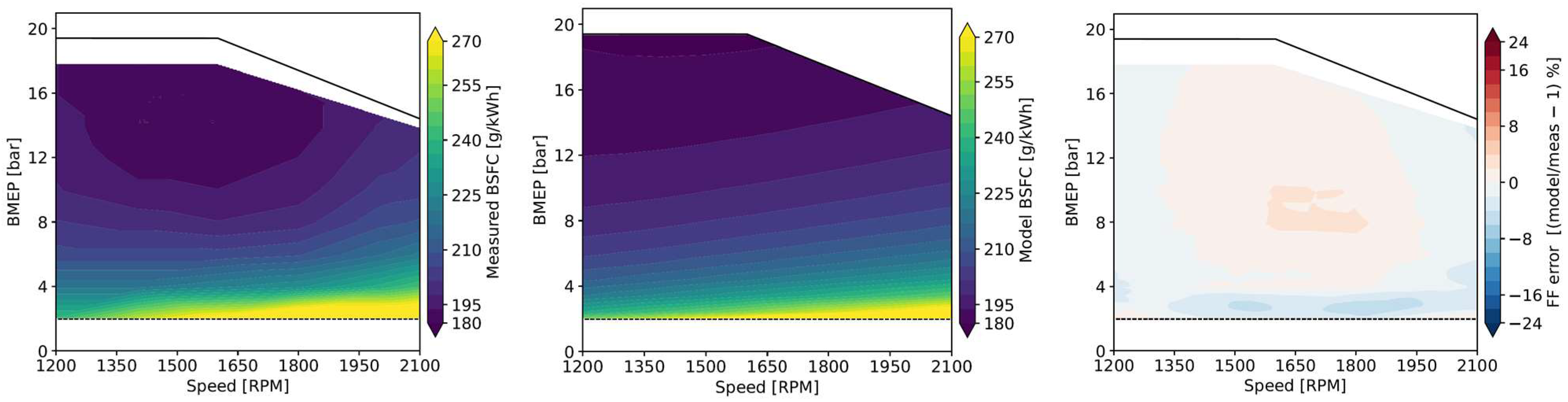
For modern turbocharged direct-injection diesel engines, ISFC is nearly constant with load [19]. Turbocharger sizing, common-rail injection pressure, and emissions management together ensure excess air across the full load range, so combustion quality does not degrade as rated BMEP is approached. The BSFC map is therefore open on the high-load side: contours do not close to the right of the efficiency island, and no load-dependent correction to ISFC is required for engines of current Tier 4 Final/Euro VI/Stage V standards.

Injection timing is often retarded from the optimal efficiency settings in order to reduce emissions. This is done selectively at points of the speed–load map where the best trade-off can be obtained between efficiency and emissions, making it a vehicle-specific calibration exercise that is impossible to track generically for a whole family of engines. In this method the engine’s minimum BSFC is taken as a primary input to the BSFC map. It is usually obtainable, and it is assumed to reflect the degree of emissions-driven timing retardation that prevails across the operating map. The degree of mismatch resulting from this assumption is included in the errors plotted in Section 3.2.

Along the speed axis, ISFC is not constant. In a four-stroke engine the combustion and expansion events occupy a fixed crank-angle window regardless of speed, so the corresponding real time scales inversely with engine speed. At low piston speed the combustion gases remain in contact with the cylinder walls for longer at near-peak temperature, and the Woschni convective heat transfer rate, which scales approximately as S_p^0.8, acts for a proportionally greater fraction of the cycle [25]. The net result is that the fraction of fuel energy rejected to coolant increases as piston speed falls, raising ISFC at low speed [19]. This competes with the rise in FMEP at high speed: the two mechanisms together produce a minimum in BSFC at an intermediate piston speed S_p,opt, which is the familiar efficiency sweet spot.

A first-order model for the speed dependency of ISFC is

$$ISFC\left(S_p\right)={ISFC}_0· (1+A_{sth}/S_P),$$

(11)

where ISFC₀ is the high-speed asymptote of indicated specific fuel consumption, and A_sth is a calibration constant with units of m/s representing the heat-transfer loss at low piston speed. The form (1 + A_sth/S_p) is a first-order approximation to the true heat-transfer fraction. The Woschni power-law S_p^−0.2 and the simpler inverse form differ by less than 5% across the practical operating range of 800–2500 RPM for off-highway and military engine families. The simpler form has the advantage that A_sth carries a direct physical interpretation as the piston speed at which the heat-transfer correction doubles ISFC relative to its high-speed asymptote [25].

2.16. Fuel Flow Equation

The fuel flow rate is obtained from the definition of ISFC. In a four-stroke engine, indicated power is

$$P_{ind}={IMEP}_{net}· V_d·{\displaystyle \frac{N}{2}},$$

(12)

where N is engine speed in rev/s, and the factor of 2 reflects the four-stroke cycle.

Multiplying Equation (12) by ISFC and substituting Equations (7)–(11) yields

$${\mathrm{ṁ}}_f \left(N, BMEP\right)={ISFC}_0· \left(1+{\displaystyle \frac{A_{sth}}{S_p}}\right)·\left(BMEP+FMEP\left(S_p\right)\right)·V_d· {\displaystyle \frac{N}{2}},$$

(13)

where ṁf is fuel mass flow rate in g/h; N is engine speed in rev/s; and V_d is total displacement in litres. In practical engineering units, with BMEP and FMEP in bar, V_d in litres, N in RPM, and ISFC₀ in g/kWh, Equation (13) becomes

$${\mathrm{ṁ}}_f={\displaystyle \frac{{ISFC}_0·\left(1+\frac{A_{sth}}{S_p}\right)·\left(BMEP+FMEP\left(S_p\right)\right)·V_d·N}{1200}}.$$

(14)

The fuel flow formulation is well-behaved at all engine speeds. At BMEP = 0 (zero-torque idle), Equation (14) gives

$${\mathrm{ṁ}}_{f,0}={\displaystyle \frac{{ISFC}_0·\left(1+\frac{A_{sth}}{S_p}\right)·\left(FMEP\left(S_p\right)\right)·V_d·N}{1200}},$$

(15)

which is positive and finite: the engine consumes fuel at idle to overcome its own friction. In the motoring condition (BMEP < 0, where the engine torque is reversed), fuel flow falls below the idle value and crosses zero at BMEP = −FMEP(S_p), the theoretical motoring threshold. Whether fuel is cut in a real engine at this point depends on the fuel management strategy, but the model is non-singular throughout and is consistent with the requirements of powertrain simulation.

2.17. Minimum BSFC

ISFC₀ and A_sth are not free parameters to be fitted independently; both are determined by the location of the minimum-BSFC operating point (BMEP_opt, S_p,opt) and the value of BSFC_min at that point. Evaluating Equation (13) at the minimum gives

$${BSFC}_{min}={\mathrm{ṁ}}_f\left(S_{p,opt},{BMEP}_{opt}\right)·1200/({BMEP}_{opt}·V_d·N_{opt}).$$

(16)

Solving for ISFC₀ yields

$${ISFC}_0={\displaystyle \frac{{BSFC}_{min}·{BMEP}_{opt}}{\left(1+\frac{A_{sth}}{S_{p,opt}}\right)·\left({BMEP}_{opt}+{FMEP}_{opt}\right)}}.$$

(17)

Similarly, A_sth is determined by requiring that the partial derivative of BSFC/BMEP with respect to S_p be zero at S_p,opt, giving

$$A_{sth}={\displaystyle \frac{C_1·S_{p,opt}^2}{\left({BMEP}_{opt}+C_0\right)}}.$$

(18)

BSFC_min is therefore a direct scaling parameter for the entire fuel flow surface: every value of BSFC is proportional to it. Where a published datasheet value is available it is substituted directly; where none is available, the regression in Section 2.11 supplies an estimate from per-cylinder displacement. In either case ISFC₀ is not an independently fitted parameter.

2.18. BSFC as a Derived Quantity

Wherever brake power P_b is non-zero, BSFC follows directly from the fuel flow rate:

$$BSFC\left(N,BMEP\right) = {\mathrm{ṁ}}_f\left(\mathrm{N},BMEP\right)·1200/(BMEP·V_d·N).$$

(19)

Substituting Equation (14) into Equation (19) and simplifying gives

$$BSFC={ISFC}_0·\left(1+{\displaystyle \frac{A_{sth}}{S_p}}\right)·\left(1+{\displaystyle \frac{FMEP\left(S_p\right)}{BMEP}}\right).$$

(20)

At low BMEP, FMEP/BMEP is large and BSFC is high; as BMEP increases, FMEP/BMEP diminishes and BSFC falls. Along the speed axis, the (1 + A_sth/S_p) term raises BSFC at low speed, while FMEP(S_p) raises it at high speed. The two mechanisms together produce a closed contour minimum at (BMEP_opt, S_p,opt) by construction. The surface is open on the high-load side, consistent with the absence of a smoke-limit combustion degradation mechanism in modern turbocharged CI engines of Tier 4 Final/Stage V standards.

The model has four calibration parameters: C₀, C₁, C₂, and BSFC_min. The bore-to-stroke ratio κ is a family constant, not a free parameter. These parameters are optimized using Excel Solver when matching a synthesized engine to a known engine’s BSFC map, or default values are calculated when synthesizing an engine from scratch.

In practice, to improve numerical conditioning when using the Excel Solver add-in, the coefficients are not optimized directly. Instead, the Solver adjusts FMEP evaluated at three reference piston speeds: C_f1 = FMEP (1 m/s), C_f5 = FMEP (5 m/s), and C_f10 = FMEP (10 m/s), as well as the minimum BSFC. The three polynomial coefficients C₀, C₁, and C₂ are then recovered by matrix inversion from these three point values. The equivalent Solver parameter set is therefore {BSFC_min, C_f1, C_f5, C_f10}. Calibration of default values is described in Section 3.

3. Results

3.1. Engine Synthesis for Applications

The engine synthesis laid out in Section 2 determines an engine specification, comprising displacement, cylinder count, rated speed, torque curve, and the two-dimensional BSFC map, based on required power output, engine family (f = f1, f2, f3 or f4 for the four families), and a choice of more or fewer cylinders where more than one cylinder count is appropriate. Recalculation of the complete synthesis chain completes in under 50 ms on a standard laptop (median 27 ms across six runs on a Dell XPS 15, Intel Core i7-8750H @ 2.20 GHz, 6-core, 32 GB RAM, Windows 11, with automatic calculation disabled in Microsoft Excel).

The synthesis does not target any individual engine; rather, it produces a specification that falls within the performance envelope of the commercial population of commercial diesel engines and therefore represents a realistic and achievable design, with the ability to adjust the scale of the engine continuously for the purpose of trade studies.

To demonstrate the synthesis workflow, engines were synthesized for two military vehicles. In [26] by the same author, hybrid powertrains were proposed for two UK Army tactical wheeled vehicles, the Foxhound and the Boxer, to provide power for the largest High-Energy Laser (HEL) weapons that each platform could carry. The key sizing specification for the hybrids is the rated power, as this determines the power for the HELs. Engines were synthesized for both platforms, with two choices for cylinder count in each case. Figure 11 and Figure 12 show the torque curves and operating envelopes for the baseline engines now in use in the Foxhound and Boxer vehicles, synthesized using the method of this paper to match the published power and torque of the current engines. Also shown are the proposed hybrid options with alternative 4- and 6-cylinder engines (Foxhound) and 8- and 12-cylinder engines (Boxer), synthesized to deliver the required power for hybrid platforms to carry HELs—which requires more power than the current platforms provide, increasing from 160 kW to 228 kW for Foxhound and from 600 to 704 kW for Boxer. The specifications are given in

Table 7. Synthesized engine specifications for Foxhound and Boxer vehicle platforms. Rated power parameters at maximum continuous speed; peak-torque parameters at peak-torque speed. All values derived from the physics-based synthesis model (Section 2).

				Rated Power			Peak Torque
Engine	Cyl	Dcyl (L)	Vd (L)	P (kW)	N (rpm)	BMEP (bar)	T (Nm)	N (rpm)	BMEP (bar)	Min BSFC (g/kWh)
Fx Baseline	6	0.533	3.2	160	3600	16.67	499	2000	19.60	218
Fx HEL 4-cyl	4	1.443	5.8	228	2370	20.00	1148	1533	25.00	200
Fx HEL 6-cyl	6	0.786	4.7	228	2902	20.00	938	1877	25.00	210
Bx Baseline	8	1.988	15.9	600	2300	19.69	2999	1500	23.70	195
Bx HEL 8-cyl	8	2.768	22.1	704	1907	20.00	4406	1234	25.00	191
Bx HEL 12-cyl	12	1.507	18.1	704	2336	20.00	3598	1511	25.00	199

Foxhound Baseline: Engine parameters from Steyr-sourced specifications. Boxer Baseline: MTU 8V 199-series parameters.

. A higher cylinder count requires smaller cylinders, which means that the engine will reach higher RPM before the piston speed limit is exceeded. The 8-cylinder engine runs up to a higher speed but has less peak torque than a 6-cylinder engine of the same power output. The same applies from 6 cylinders to 4 cylinders for the Foxhound. Both options satisfy the power requirement for the Foxhound, but considerations such as cost, weight, package space or NVH might drive the ultimate choice between the two. Figure 13 shows synthesized fuel flow and BSFC for the 12-cylinder version.

The synthesized engine specifications were compared with the dataset of engines introduced in Section 2. Figure 1, Figure 2, Figure 3, Figure 4, Figure 5, Figure 6 and Figure 7 and Figure 10 each overlay the synthesized Foxhound and Boxer engines on scatter plots of the compiled dataset. In each case, the synthesized values fall within the populated region of the scatter, demonstrating that the synthesis outputs are consistent with the performance and efficiency capabilities of commercially available engines. The model is not required to predict any individual engine’s parameters; the scatter visible in every figure is inherent to the real population, reflecting genuine diversity in design philosophy, turbocharger specification, calibration, and market positioning.

Where a baseline engine is constrained to match a known production unit, which happened for the Steyr 6-cylinder for Foxhound and the MTU 8V 199 for Boxer, the corresponding points fall below the S_p,max envelope, consistent partly with real engines being specified conservatively and partly with the sub-optimal performance of older legacy engine families. Where hybrid variants are synthesized without datasheet constraints, they fall on or close to the family envelope by construction, representing the upper performance boundary that current manufacturing technology can credibly deliver, which is the appropriate target when specifying a new engine for a future platform.

In Figure 1 the Foxhound baseline point sits at approximately 16.7 bar rather than the 20 bar synthesis assumption, reflecting the actual rated BMEP of the Steyr engine; the synthesis chain adopts 20 bar as achievable for a new-build engine, so this offset is expected. In Figure 5, the hybrid variants fall precisely on the 10.56 m/s envelope line because rated speed is determined analytically from S_p,max by Equation (1).

3.2. Fuel Efficiency Estimation

Figure 14, Figure 15, Figure 16 and Figure 17 show the BSFC of four engines from the comparator database, firstly as measured, secondly as modelled using the method of this paper, and thirdly showing the error in per cent between the two. Point-by-point errors are generally contained within the +−5% range, indicating that the model has reasonable capability in tracking the characteristics of the surface.

Table 8. Solver-optimized FMEP values and minimum BSFC for all calibrated engines. C_f1, C_f5, and C_f10 denote FMEP (bar) at mean piston speeds of 1, 5, and 10 m/s respectively. Family: f1 = Automotive, f2 = Truck, f3 = Off-Highway.

Engine	Family	BSFCmin (g/kWh)	Cf1 (bar)	Cf5 (bar)	Cf10 (bar)
CI37	f1	244.04	0.7972	0.8738	1.2320
CI54	f1	241.62	2.4139	3.0031	3.9103
CI60	f1	216.64	0.8733	1.5232	2.8065
CI67	f1	205.93	1.2299	1.7496	2.7547
CI88	f1	196.55	1.4350	1.8372	3.0531
CI92	f1	187.99	1.7028	1.8598	2.8731
CIEPA_BMW_3L	f1	203.46	0.1174	1.0386	1.9913
EPA_GM_3L	f1	205.12	0.2643	0.4147	1.0448
CI119	f3	220.28	0.3640	0.3740	0.6035
CI171	f2	188.42	0.4541	0.5926	1.0472
CI205	f2	189.47	0.0253	0.5332	1.1582
CI246	f2	196.03	0.0100	0.4377	0.7834
CI250	f2	188.20	0.0100	0.5875	1.2508
CI321	f2	191.48	0.6852	0.6952	1.3266
CI324	f2	193.39	0.6639	0.6739	1.1917
CI330	f2	189.15	0.0100	0.5556	1.2011
Marinoni	f1	212.16	0.4119	0.9675	3.7812
Moghadisi	f2	207.63	0.8023	0.8123	1.7768
Ratislav	f2	205.54	0.8024	0.8124	0.8324
Fendt211	f3	187.19	1.8863	1.8963	3.3167
Fendt314	f3	211.42	1.1771	1.1871	2.6241
Fendt722	f3	205.91	0.0100	0.0200	0.0400
Fendt724	f3	202.97	0.0100	0.0200	0.0400
Mean (f1)		—	1.0273	1.4742	2.6052
Mean (f2–f3)		—	0.4936	0.6570	1.2280

shows the coefficients C_f1, C_f5, and C_f10 (FMEP, bar, at 1, 5, and 10 m/s mean piston speed) used by the model to fit each engine. The model is reproduced in Excel workbooks [14], and Excel Solver was used to determine the coefficients. Of the 23 comparator engines for which BSFC maps were found, all five that were post-2020 showed little or no sign of BSFC worsening at maximum torque; i.e., BSFC at maximum torque was close to the minimum BSFC overall. However, the older engines did show such signs, which are attributed to overfueling leading to inefficient combustion in engines where emissions requirements were less stringent. This phenomenon appears in a BSFC map as a tendency to worsen BSFC in the last stages of torque increase, at any given RPM, and this is visible in some of the older BSFC maps used in this paper. Modern turbocharged DI diesel engines operate with overall excess air (λ > 1) across the full load range ([19], Ch. 15), so combustion efficiency does not degrade as maximum torque is approached. Accordingly, since the synthesis model is intended for modern engine specifications only, the ISFC calculations in Section 2 do not include any term with freedom to follow a worsening of efficiency with loads above the point of minimum BSFC, and it is assumed that minimum BSFC for modern turbocharged diesel engines, excluding de-rated versions, may be considered to take place at the peak-torque operating point.

The mean values are adopted for engine synthesis for Family 1 and for Families 2–4. Figure 18 shows the FMEP values graphically.

3.3. Application to Hybrid Powertrain Screening

Figure 19 shows a Foxhound engine in a powertrain model generated by ePOP Concept, from Tull de Salis [27]. It is included here to illustrate the practical application of a fast simulation method for powertrain architecture screening, which could benefit from the improved BSFC estimation method of this paper.

The analysis of [27] predicts fuel consumption savings if applying a parallel hybrid architecture to a Foxhound tactical wheeled vehicle of the British Army but a fuel consumption increase if a serial hybrid is deployed, with ICE-only (internal combustion engine) as baseline. These results are obtained against a drive cycle representing a 24 h combat mission. However, the analysis used a constant-BSFC assumption for the engines, which were hypothetical versions scaled to fit each architecture, and although it included the effects of engine-off operation, it was not able to reflect the effects of BSFC changes due to engine scaling. With the methods of this paper, which are very rapid in calculation and require no iteration to arrive at each result, it would be possible to enhance the analysis in [27] without requiring additional data collection, user configuration, or computation time beyond that which the existing analysis already demands.

3.4. Response to Engine Downsizing

Figure 20 shows the effects of applying a drive cycle to the measured and modelled BSFC maps of four engines. The drive cycle is adapted from the World Harmonized Stationary Cycle (WHSC) [28], shown in Figure 21, which is scalable to fit the capacity of any engine. Normalized torque ranges from 0 for the minimum to 100 for the maximum, within the engine’s operating range at a given RPM. Normalized RPM ranges from 0 at idle RPM to 100 at the maximum RPM of the engine. The weighted fuel efficiency over the drive cycle is calculated and expressed as BSFC. The minimum BSFC of the engine is shown in the first pair of bars, allowing a comparison of the minimum seen on the published source engine map and the minimum in the fitted model. For the other three pairs of bars, the torque points of the WHSC cycle were scaled at proportions of 1.0, 0.8 and 0.6 and applied to the measured and modelled BSFC maps. The purpose of the comparison is to simulate the effect of upsizing or downsizing an engine for a fixed duty cycle, but instead of changing the engine, the duty cycle is scaled. Since the source data are fixed and cannot be modified for a different engine size, the duty cycle is scaled as a proxy for changing the engine size. The BSFC naturally increases from the engine minimum because the other points on the BSFC map are by definition higher than the minimum. The most efficient match is where the drive cycle is at full scale (1.0) since it uses higher BMEP points on the map. As the duty cycle is scaled down, the BSFC worsens (increases), simulating an engine that is oversized for its application. The figure shows that just as the measured BSFC worsens with decreasing scale of load, so the modelled BSFC also worsens in approximately the same proportion. The change in the measured results illustrates the main advantage of applying a synthesized BSFC map instead of using a constant-BSFC assumption for an unknown engine, as it informs an architecture selection process about the effects of engine downsizing, and specifically hybridization, on the fuel efficiency of the vehicle. The change in the modelled results validates the suitability of the model for tracking this phenomenon.

4. Discussion

The physical basis of the synthesis distinguishes it from prior empirical correlations in the literature. Heywood and Welling [7] and Chon and Heywood [6] developed regression-based correlations for spark-ignition engines, demonstrating that performance normalizes well against piston speed and total piston area. The present work extends this framing to compression-ignition engines across four application families, replacing regression against arbitrary polynomial terms with relationships derived from first principles; the rated-speed model follows directly from the mean-piston-speed ceiling and cylinder geometry; the BSFCmin displacement dependence follows from the surface-to-volume scaling of combustion chamber heat transfer; and the BSFC map shape follows from the competing effects of wall heat transfer and friction on indicated and brake efficiency respectively. As a result, each parameter in the synthesis carries a physical interpretation that constrains its behaviour and makes the model physically consistent outside the calibration range. Suijs and Verhelst [8], working with large-bore stationary spark-ignition engines, similarly adopted physics-based scaling to constrain their correlations. The present work reaches the same conclusion for diesel powertrains across a much wider application range.

The stratification into four engine families is a necessary feature of the method rather than an arbitrary choice. The families differ systematically in bore-to-stroke ratio, piston speed ceiling, and FMEP level, and pooling data across families would obscure these differences and degrade predictive accuracy. The mean FMEP values shown in Figure 18 illustrate this directly: f1 automotive engines show substantially higher friction at high piston speeds than f2 and f3 engines, reflecting their smaller cylinder bores, higher operating speeds, and more aggressive friction reduction targets, driven by passenger car CO₂ regulations. Applying f1 FMEP coefficients to an f3 engine synthesis would produce a map whose shape is qualitatively correct but quantitatively wrong at the operating speeds most relevant to agricultural and construction applications.

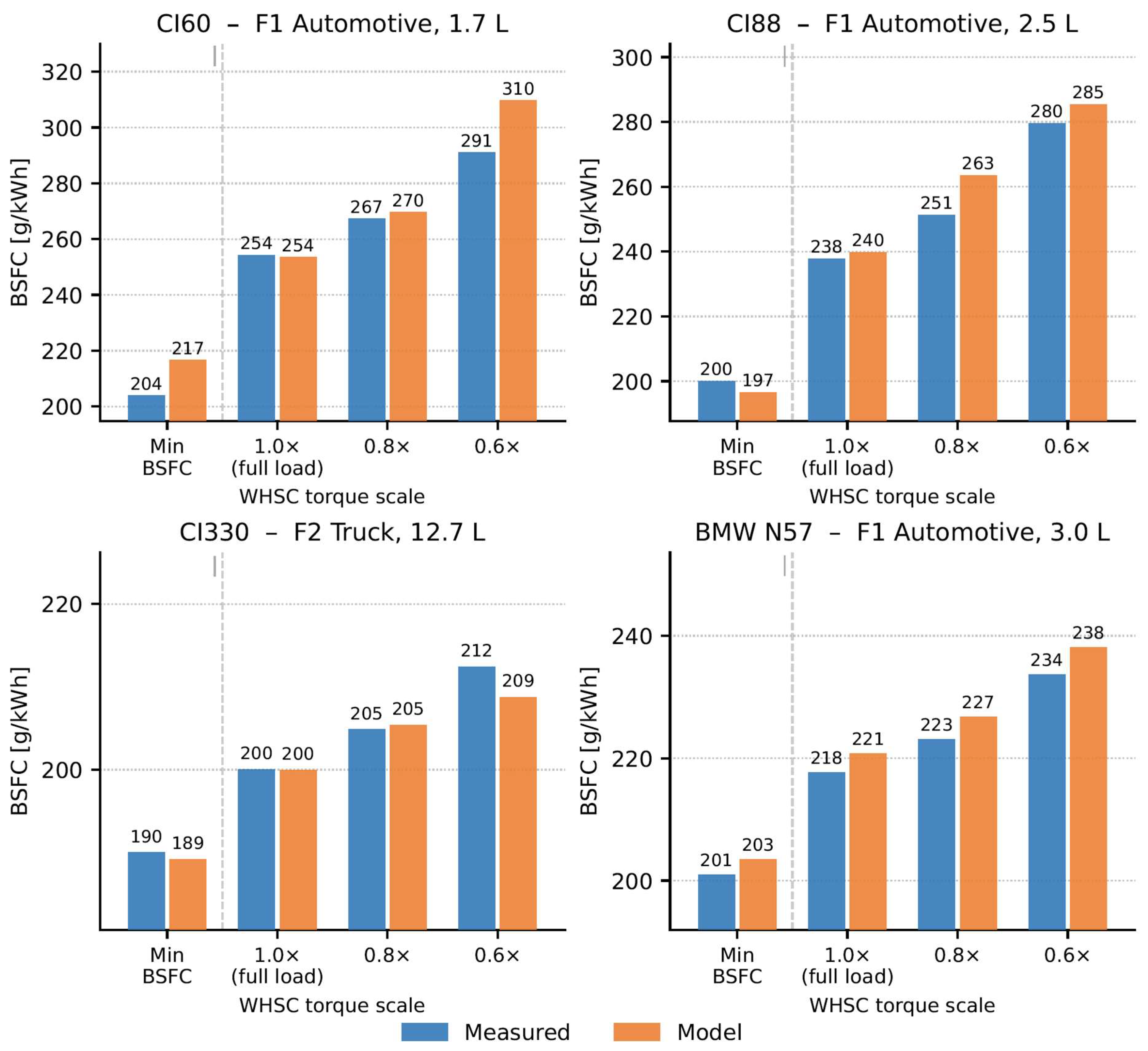
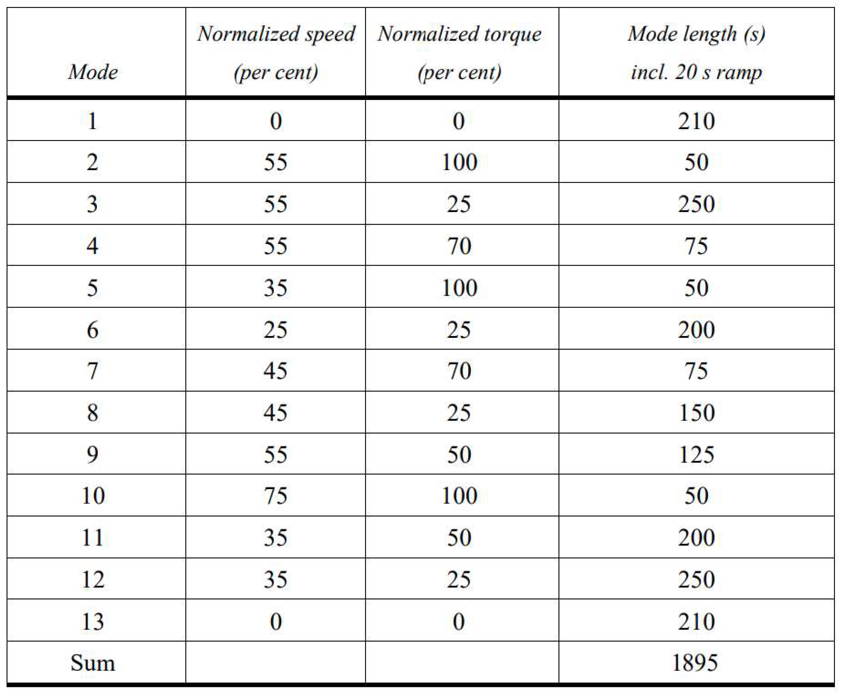
The validation in Section 3.4 addresses a specific and important concern: not merely whether the synthesized map resembles the measured map visually, but whether it responds correctly to changes in the load distribution imposed on it. This is the property that matters for hybrid architecture trade studies, where the central question is how BSFC changes when an engine is downsized and forced to operate at higher load for a given duty cycle, or when engine-off operation shifts load to periods of higher battery state of charge. The WHSC-based comparison in Figure 20 shows that the model correctly reproduces the direction and approximate magnitude of the BSFC change as the torque scale is reduced from 1.0× to 0.6× across all four comparator engines. The agreement is closest for CI330 and the BMW N57, where the model tracks the measured trend to within 3 g/kWh across all three load conditions. For CI60 and CI88, the agreement at 1.0× and 0.8× is good, but the model slightly overpredicts the rate of BSFC increase at 0.6×. This is consistent with the nature of the calibration data: the ADVISOR (version 2003-00) maps from which CI60 and CI88 are drawn extend to lower BMEP values than most modern measured maps, and the model’s extrapolation into the low-load region relies on the ISFC heat-transfer term rather than directly measured data. The divergence at 0.6× torque scale is therefore expected behaviour, not a model failure, and the magnitude (approximately 15–20 g/kWh at the most extreme condition) remains within an acceptable range for concept-phase screening.

The limitation acknowledged in Section 3.3—that the earlier analysis of [27] used a constant-BSFC assumption—illustrates an important point about the value of the present method. A constant-BSFC model correctly captures energy substitution effects in plug-in hybrid architectures, where electrical energy from an external source displaces fuel energy regardless of operating point. It does not, however, capture the fuel efficiency benefits that arise from operating a smaller engine at higher load—load-point shifting—which is one of the two primary mechanisms available to non-plug-in hybrid architectures operating away from fixed bases. For military and off-highway applications, where charging infrastructure is unavailable during operations, non-plug-in hybridization is the viable electrification path, and load-point shifting is therefore a central performance claim. A synthesis method that supports continuous engine scaling and provides a map that responds correctly to load changes is accordingly a more appropriate tool for this application class than a constant-BSFC assumption, even if the absolute accuracy of the BSFC map is modest.

The method has several limitations. First, it does not model transient behaviour: the maps represent steady-state operation, and transient fuel enrichment, turbocharger lag, and after-treatment thermal management effects are not captured. For the concept-phase architecture screening for which the method is designed, this is acceptable, as the steady-state map provides the correct average fuel consumption for a given duty-cycle distribution, but users should not apply the method to predict instantaneous fuel flow during rapid transients. Second, the method assumes that BSFCmin occurs at the peak-torque operating point for modern Tier 4 Final and Stage V engines, consistent with the observation that all five post-2020 engines in the comparator dataset showed negligible BSFC degradation at maximum torque. For older engines, or engines calibrated to less stringent emissions standards where overfueling at high load was accepted, this assumption will overpredict efficiency at high load. Third, the cylinder count thresholds of Table 1 reflect the current production population and are not analytically derived; they should be reviewed if the method is applied to engine families significantly outside the 30–800 kW range, where different architectural conventions may apply. Fourth, the method treats bore-to-stroke ratio as a family constant, whereas real engines within a family span a range of κ values. This introduces a systematic uncertainty in the stroke and therefore the friction model, though the sensitivity is modest: a 10% variation in κ produces approximately a 3% change in rated speed prediction via Equation (1), which is small relative to the scatter in the calibration data.

Two directions merit future attention. First, the military family (f4) is currently supported for engine specification synthesis but lacks calibrated BSFC maps, because no measured f4 maps could be identified in the open literature. The FMEP coefficients adopted for f4 synthesis are taken from the f2–f3 mean, which is a reasonable engineering approximation but not a validated result. Acquisition of measured BSFC data for representative military diesel engines—even a single well-documented map—would allow proper calibration of the f4 FMEP model. Second, the BSFCmin correlation of Equation (6) uses a fixed asymptote r = 154 g/kWh anchored by Uyehara’s large-displacement data from 1987. Modern large-bore marine and locomotive engines have advanced significantly since then, and a contemporary survey of large-cylinder minimum BSFC values would allow this asymptote to be updated with greater confidence. Neither extension alters the structure of the synthesis chain, which is designed to accommodate substitution of improved parameters at any step. Both limitations reflect the same underlying constraint: the present analysis is bounded by the poor availability of published BSFC maps for real engines, and the method could be enhanced significantly, in its calibration if not its structure, by access to a larger pool of engine data.

5. Conclusions

A method has been presented for synthesizing a complete diesel engine specification, comprising displacement, cylinder count, rated speed, torque curve, and two-dimensional BSFC map, from two inputs: required power output and application family.

The method requires no measured engine data beyond publicly available sources and is non-iterative: each engine synthesis executes a fixed sequence of closed-form equations requiring no convergence loops, completing in under 50 ms on standard hardware.

The key quantitative results are as follows. Synthesized specifications fall within the populated scatter of each family across all primary parameters: rated BMEP, peak-torque BMEP, rated speed, per-cylinder displacement, and minimum BSFC. WHSC-based validation across four comparator engines confirms that the synthesized maps track the direction and approximate magnitude of BSFC change under load scaling from 1.0× to 0.6× of rated torque, with agreement to within 3 g/kWh for CI330 and BMW N57, and a maximum divergence of approximately 15–20 g/kWh at the most extreme load condition for CI60 and CI88. The family stratification into four application classes—automotive/light commercial (f1), medium and heavy-duty truck (f2), off-highway agricultural and construction (f3), and military (f4)—is shown to be necessary: FMEP levels and piston speed ceilings differ systematically across families, and pooling data across them would degrade predictive accuracy.

The method’s primary contribution is that each parameter carries a physical interpretation derived from first principles rather than a fitted polynomial, making the model physically consistent outside its calibration range. This is particularly relevant for hybrid architecture trade studies in off-highway and military applications, where non-plug-in hybridization is the viable electrification path and the efficiency benefit of load-point shifting—which a constant-BSFC assumption cannot capture—is a central performance claim.

The method is intended for concept-phase use. It does not model transient behaviour, assumes BSFCmin at the peak-torque point consistent with modern Tier 4 Final and Stage V calibrations, and treats bore-to-stroke ratio as a family constant. The military family (f4) synthesis is supported for engine specification but lacks validated BSFC maps. These limitations are consistent with concept-phase screening requirements and do not affect the method’s suitability for its intended purpose.