Abstract
This study addresses the condition monitoring of rolling bearings by applying robust linear regression to statistically derived features from vibration data. Four datasets of acceleration signals were collected under varying operating conditions: aligned and misaligned bearings at rotational speeds of 1000 rpm and 1500 rpm. From each signal, key statistical indicators were extracted, including root mean square (RMS), skewness, kurtosis and crest factor, to capture signal characteristics that were relevant to fault detection. To follow-up, we applied the Kolmogorov–Smirnov test to assess data normality and the results confirmed significant deviations from a Gaussian distribution, motivating the use of robust regression techniques for further investigations. The regression model created incorporated rotational speed and alignment conditions as predictors of acceleration and the results indicated that while the coefficient associated with misalignment suggested a possible increase in acceleration (~1.115 units), statistical testing (p = 0.5233) indicated that neither speed nor alignment had a significant influence on the measured vibration levels within the dataset. The findings suggest that under the tested conditions, misalignment does not manifest as a strong linear change in acceleration magnitude, and the study underscores the importance of robust modeling techniques and feature selection in the condition monitoring of rotating machinery.
1. Introduction
Bearings are one of the most important constituents of a mechanical transmission, and are used to support rotating parts and reduce friction. Most of the studies related to bearing functioning study load capacity, lubrication techniques, wear resistance and noise generation. The lubrication regime is often a focus, including studies on oil flow and temperatures. Because most of the damages to roller bearings are due to wear, whether they are determined by lubricant failure or contamination or by normal fatigue, now, studies focus on predicting bearing failures in advance, with the use of vibration or temperature analysis, advanced techniques such as deep learning and neural networks or advanced mathematical tools, such as multiple linear regression (MLR), with the use of statistical inference and model building.
Linear regression models have long been used in statistical analysis for their simplicity and interpretability. In the context of bearing condition monitoring, linear regression can offer valuable insights into the relationships between vibration characteristics and bearing health. However, traditional linear regression models often struggle with outliers, multicollinearity and noise, which are common in vibration datasets. As a result, a robust regression framework is required to address these issues and improve the model’s performance.
Over the past few decades, numerous studies have explored the use of vibration-based techniques for bearing fault detection. Early research focused on the extraction of simple features, such as root mean square (RMS) and peak-to-peak amplitude, with a view to detecting major faults such as outer race, inner race and ball bearing defects. More recently, studies have moved towards advanced techniques such as wavelet transform [1,2], empirical mode decomposition [3,4] and deep learning-based methods, according to [5,6,7,8]. However, despite significant progress in the area, the challenge of selecting the right features and developing models that are both accurate and computationally efficient remains. Recent advancements in robust regression techniques, such as least absolute deviations (LAD) regression and weighted regression models, have shown promise in providing more reliable estimates in the presence of noise and outliers.
Several studies have highlighted the limitations of standard regression techniques when applied to vibration-based fault detection. For instance, Daoud (2017) [9] noted that traditional regression methods are often hindered by multicollinearity in high-dimensional vibration datasets. Other researchers, such as Giloni et al. (2006) [10] and Tian and Wang (2021) [11], have explored the use of robust regression methods, such as LAD regression, that offer improved resistance to the effects of noise and outliers. Despite these advancements, there remains a lack of comprehensive studies that systematically investigate the effectiveness of robust regression in bearing condition monitoring, particularly when compared to more traditional approaches.
Yan et al. [12] proposed an adaptive regression model to estimate the remaining life of a bearing, by using an elbow point detection design to improve the prognostic performance. The paper showed that the suggested method can effectively determine the time to start the prediction and can calibrate the degradation regression model dynamically, according to the evolving degradation trend in the health indicator (HI).
While there is a wide array of anomaly detection algorithms for bearing fault identification, few studies utilize the specific, simple setup presented in our work. The decision to use one analysis method or another is difficult, as it is amplified by the varying experimental setups, which often do not allow for a direct comparison of results under consistent conditions.
In terms of methodology, our study aims to determine whether bearing faults can be detected using simple, computationally efficient models and what the difficulties in applying an appropriate analysis method are. This is particularly important, given that numerous studies have shown that bearing operation is a nonlinear and non-stationary process, which makes it challenging to accurately assess their performance and functional condition [13,14]. To this end, we chose to investigate the limitation of applying robust regression analysis, as statistical methods are among the widely recognized approaches. Therefore, regression techniques are one of the most used methods to evaluate bearing functioning, its remaining life cycle or high influence parameters [15,16]. To that end, the use of multiple regressions, as an extension of linear regression, takes into account more than one independent variable as input, to predict a single output variable. Such a technique can only be effectively applied if the deviation of any data point from the fitted line exceeds the maximum allowable error for the measured variable. To that end, the first step is to perform a baseline diagnosis with the use of informative predictors such as RMS (root mean square), kurtosis, skewness and crest factor, as part of the vibration analysis and condition monitoring goals, highlighting the comparative values between aligned and misaligned functional bearing, while running at 1000 rpm and 1500 rpm. The use of time domain analysis contributed to the overall measure of the signal’s energy, detection of impulsive events in the endogenous variable, like pitting, spalling or a crack in the bearing, or detection of non-uniform loading or misalignment.
Given that feature extraction introduces numerical complexity, our study also highlights the challenges derived from the data processing on fault detection performance. Our findings show that, for certain experimental methods, choosing the appropriate method is challenging and the results can be inconclusive for pointing out certain statements, such as the effect of certain degrees of misalignment on bearing functioning.
The second step was to inspect the variable variation, then proceed with the linear regression itself. There were several attempts to identify a suitable regression method, taking into account the Gaussian or non-Gaussian distribution of data. It was assumed to be a normal distribution of acceleration; it was verified and, in the follow-up, we chose a more appropriate regression model.
Hence, the main purpose of this study is to investigate the application of robust linear regression for bearing condition monitoring, focusing on identifying key predictors for fault detection under different operational conditions. Specifically, we examine the bearing behavior in both aligned and misaligned states at two distinct rotational speeds (1000 rpm and 1500 rpm). By employing robust regression techniques, we aim to model how changes in bearing misalignments and functioning speed affect the acceleration values. Hence, the acceleration is considered to be the dependent variable, and misalignment and speed are the independent ones: the former is a quantitative parameter and the latter is the continuous variable. This research contributes to the growing body of knowledge on predictive maintenance, offering valuable insights for industries such as automotive, aerospace and manufacturing, where bearing health is critical to operational performance.
The study is situated within recent advancements in machine learning and statistical methods for condition monitoring, where feature extraction and model robustness are key to improving fault diagnosis accuracy, and it concluded that the datasets used for analysis showed a faulty bearing submitted to tests, with problems caused by wear and the low-to-minimal influence of bearing alignment and functional speed on the resulting acceleration values. Also, the absence of strong linear effects highlights the complexity of fault diagnosis in bearing systems, suggesting that additional nonlinear or time-series methods could be explored in future work. Our findings emphasize the importance of carefully chosen methodologies and the selection of relevant features in condition monitoring tasks, contributing to the ongoing evolution of data-driven predictive maintenance strategies.
2. Materials and Methods
The physical configuration used during experimental tests comprises a control unit, a mechanical assembly and a computer, as depicted in Figure 1.
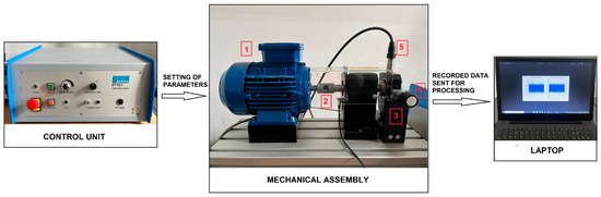
Figure 1.
Configuration of experimental setup and constituent elements.
The control unit was used to vary the functioning speed of the mechanical transmission, generating the first independent variable. The mechanical assembly comprised an electric motor (1), a flexible jaw coupling (2), a bearing seat (3) with a roller bearing, loading knob for radial forces (4) and a piezoelectric accelerometer with integral electronics (IEPE sensor), mounted in a vertical position on a threaded bore. The main characteristics of the piezoelectric accelerometer and the roller bearing are presented in Table 1.

Table 1.
Characteristics of the main elements of the mechanical assembly.
Different types of experimental tests were conducted, wherein the functioning speeds and statuses of bearing were varied, resulting in the following four cases:
- Functioning speed of 1000 rpm, aligned roller bearing;
- Functioning speed of 1000 rpm, misaligned roller bearing;
- Functioning speed of 1500 rpm, aligned roller bearing;
- Functioning speed of 1500 rpm, misaligned roller bearing.
The misalignment of the bearing was set through the loading knob of the mechanical assembly by applying a constant static load, depicted on the scale as 2.5 mm, which corresponds to a force of 100 N. Each test lasted 120 s, during which the measured data from the accelerometer (namely acceleration values) were transmitted to the laptop for further processing and analysis.
Prior to conducting the linear regression analysis, we established the physical status of the analyzed bearing, meaning whether there are damages on either of the characteristic elements, by means of time domain analysis. To that purpose, four statistical features of the measured acceleration series were determined, which are depicted in Table 2.
Table 2.
Statistical indicators used for the analysis of bearing functioning.
The details about the formulas that are used to calculate each statistical indicator within Table 2 are presented in Appendix A.
After obtaining the results for each baseline indicator, in order to assess the overall shape of the data distribution and ensure more accurate analysis, the Kolmogorov–Smirnov (KS) test was applied. This statistical test evaluates whether the dataset follows a normal distribution by defining the null hypothesis (H0), running the test itself and then interpreting the results.
To that end, we considered the sample of data: namely, acceleration values such as , , , …,. To test the hypothesis that the sample comes from a specific distribution, denoted F0 (e.g., normal distribution), against the alternative that it is from another distribution, denoted F (the empirical distribution derived from sample), where F() ≠ F0() for some ∈ R, it is calculated that the Kolmogorov–Smirnov statistic is the maximum absolute difference between the empirical cumulative distribution function (ECDF) and the theoretical cumulative distribution function (CDF) [17]:
Empirical CDF at point (where represents the i-th ordered observation) is as follows:
where
and data were sorted in ascending order as follows: .
The theoretical CDF is the following:
where represents the cumulative distribution function of the normal distribution.
In the absence of normality, multiple data transformations were performed, such as power and square root. The results were not favorable. As a consequence, taking into account the lack of Gaussian fit of data and residuals, even after several attempts to apply transformations, it was chosen to continue the study of bearing functioning by means of robust regression, which is more suitable for considering the characteristics of acceleration values.
Robust regression is also a linear regression technique that relaxes assumptions regarding outliers, handling heteroscedasticity and non-normal residuals, and it fits the model by minimizing weighted errors, using functions like bisquare.
The general equation used was as follows:
where y is the dependent variable (acceleration), x1 is the first independent variable (speed), x2 is the second independent variable (alignment), x1x2 is the interaction term between speed and alignment and ε represents the error term.
Y = β0 + β1·x1 + β2·x2 + β3·x1·x2 + ε,
Assuming that the regression output includes coefficients (denoted β0, β1, β2, β3) for the intercept, main effects and interaction, the regression equation can be written as follows:
where β0 is the intercept term (baseline acceleration when speed = 0 and alignment = “aligned”), β1 is the coefficient for speed (the effect of speed on acceleration), β2 is the coefficient for alignment (the effect of alignment on acceleration), β3 is the coefficient for the interaction between speed and alignment, Dalignment has a value of 0 for “aligned” and 1 for “misaligned” and ε represents the error term (residuals).
Acceleration = β0 + β1·speed + β2·Dalignment + β3·(speed × Dalignment) + ε,
3. Results
3.1. Time Domain Analysis Results
The results of RMS, as depicted in the calculation, indicated a value of 16.62 m/s2 in the case of the aligned bearing and 38.96 m/s2 for the misaligned one, for a functioning speed of 1000 rpm, and 31.77 m/s2 and 70.00 m/s2, respectively, for the aligned and misaligned bearings, for a functioning speed of 1500 rpm. In the case of mechanical parts, RMS values are a measure of signal magnitude, which is useful to determine, especially when dealing with time-varying parameters like acceleration. In the absence of manufacturing guidelines for the specific roller bearing, one can compare the values measured in the cases of aligned and misaligned bearings, which revealed that the misalignment condition caused an increase in RMS by more than 2.34 times at 1000 rpm and 2.2 times at 1500 rpm. At 1000 rpm, misalignment increases the RMS by a greater factor compared to 1500 rpm, even though the absolute RMS values are higher at 1500 rpm. The result here indicates that the system is more sensitive to misalignment at lower speeds in terms of the RMS increase, potentially because of the specific operating characteristics of the bearing or the system.
In terms of the calculated values of kurtosis, it resulted that is 4.15 in the case of the aligned bearing and 3.69 for the misaligned one while running at 1000 rpm, and the values at 1500 rpm are 4.33 and 3.39, respectively. According to the literature, a kurtosis value above three indicates a leptokurtic sample that is greater than that of a normal distribution, which is consistent with heavier tails, a sharp peak around the mean and more extreme outlier or impulsive values. This implies that the bearing’s vibration signal contains spikes and impulses, possibly indicating early-stage faults on bearing elements due to the wear phenomenon.
Also, the comparative display of the detailed statistical indicators before, as well as for skewness and crest factor, which are detailed in the follow-up, is depicted in Figure 2 and Figure 3.
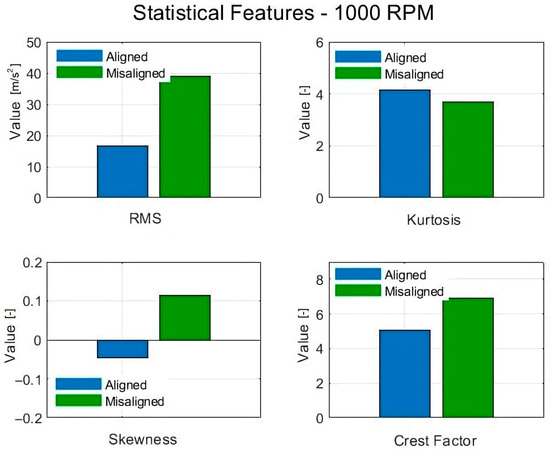
Figure 2.
Comparative statistical features (RMS, kurtosis, skewness and crest factor) for aligned and misaligned bearings at 1000 RPM.
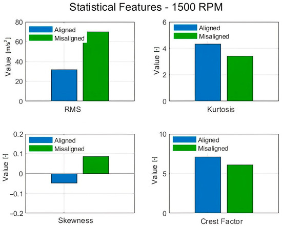
Figure 3.
Comparative statistical features (RMS, kurtosis, skewness and crest factor) for aligned and misaligned bearings at 1500 RPM.
From Figure 2 and Figure 3, it can be observed that the RMS values are higher in the case of the misaligned bearing, which is known due to the fact that this condition increases non-Gaussian characteristics. Higher values of RMS indicate larger amplitude values on average. Regarding kurtosis, the two figures show higher values for the aligned bearing, which is counterintuitive. Possible causes can reside in the type of misalignment, which determines the type of vibration response; the introduction of additional frequency components into the vibration spectrum, which might be more regular or sinusoidal; or the fact that misalignment can create a smoother and more consistent vibration pattern where periodic vibrations can be present.
From the calculation, it was determined that for the aligned and misaligned bearings, the sw is −0.04 and 0.11 while functioning at 1000 rpm, and −0.04 and 0.08 while functioning at 1500 rpm. According to [14,15], the values between −0.5 and 0.5 indicate an approximately symmetric distribution, characterized by moderate skewness, which represents an advantage for applying further regression analysis. The visual representation of acceleration distribution is depicted in Figure 4.
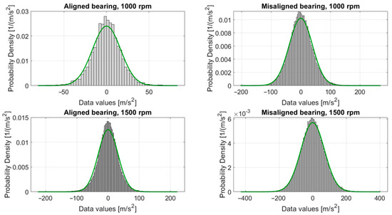
Figure 4.
Overlay of normal distribution curve on the histogram of acceleration values.
Given the negligible skewness values, that are still different from 0, the results cannot indicate with certainty that the data follow a normal distribution. Hence, to check the overall shape of the distribution and obtain more relevant results, the Kolmogorov–Smirnov (KS) test was applied. This is used to check if the data follow a normal distribution, considering the null hypothesis (H0). If h = 0 (where h is the variable used to define the result when performing hypothesis tests), we fail to reject H0, meaning the data follow a normal distribution, and if h = 1, we reject H0, meaning the data do not follow a normal distribution. Considering that the critical value of 0.016 (for the aligned bearing, at 1000 rpm) and 0.0045 (for the other three tests), was calculated according to the sample size and the significance level α = 0.05, they were compared with the determined KS statistic. Also, the empirical cumulative distribution function (ECDF) and theoretical cumulative distribution function (CDF) were displayed (Figure 5) to determine the degree of fitting of the acceleration series to the normal distribution.
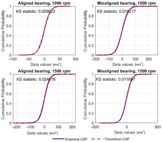
Figure 5.
Comparison of empirical and theoretical cumulative distribution function for aligned and misaligned bearing, while functioning at 1000 rpm and 1500 rpm.
From the resulting values of the KS statistics displayed in Figure 5, it can be concluded that the acceleration values do not fit a normal distribution (all four KS statistics are higher than the corresponding critical values). Even if the acceleration values do not have a Gaussian fit, one can check the residual distribution for normality in order to apply multiple linear regression analysis in the follow-up. Considering this, the Kolmogorov–Smirnov statistical method was also applied to test the residuals. The method was chosen due to the large dataset of values, and it applied a regression model to the known data (to calculate the residuals). The results also indicated that the test result was 1, which suggests that the null hypothesis (H0) is rejected and the data do not fit a normal distribution. Also, the p-value, which was used to represent the probability of observing data under the assumption of the null hypothesis, was 0.0000, which implies that it strongly rejects H0.
In the case of the fourth indicator, the crest factor, the resulting values were 5.03 and 7.10 for the aligned and misaligned bearing while functioning at 1000 rpm and, while functioning at 15,000 rpm, the crest factors were 6.92 and 6.10. Generally, the misalignment typically increases the dynamic forces on the bearing, leading to more sudden peaks in vibration, hence the higher crest factor while functioning at 1000 rpm. Also, while functioning at 1500 rpm, there were lower values observed than in the misaligned condition at 1000 rpm. This could suggest that at higher speeds, the bearing experiences slightly more transient events, due to factors like increased centrifugal forces or slight operational changes, but the bearing is still operating relatively smoothly.
3.2. Robust Regression Analysis Results
Substituting Formula (6) with the calculated values, the regression model becomes the following:
acceleration = −0.0523 + 0.00009·speed + 1.1150·Dalignment − 0.0015·(speed × Dalignment)
All the estimated coefficients are presented in Table 3, and the graphical representations of residual distribution are depicted in Figure 6 and Figure 7.
Table 3.
Estimated coefficients after applying linear regression model (robust fit).
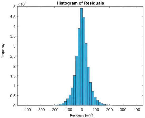
Figure 6.
Histogram of residuals after applying robust regression for aligned and misaligned bearings, while functioning at 1000 rpm and 1500 rpm.
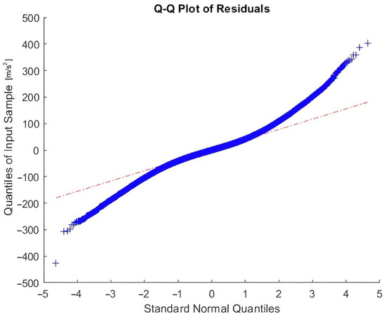
Figure 7.
Q-Q plot of residuals after applying robust regression for aligned and misaligned bearings, while functioning at 1000 rpm and 1500 rpm.
From Table 2, it can be observed that all p-values indicate the results, and predictors are not statistically significant; for example, the coefficient for speed indicates that the effect of speed on acceleration is very small (0.00009). The high p-value (0.9365) indicates that speed is not a significant predictor of acceleration in this model. Essentially, changes in speed do not have a statistically significant effect on the acceleration values, based on the current data.
Also, the coefficient for alignment status (aligned versus misaligned) suggests that, on average, misalignment might increase the acceleration by around 1.115 units. However, the p-value (0.5233) is much higher than 0.05, which indicates that the alignment condition does not have a statistically significant effect on the acceleration, considering the recorded variable at constant functioning speed.
Yet again, the small number of variables that are taken into account generated results showing that the model has a high residual error (RMS = 43.9), indicating that most of the variation in the acceleration remains unexplained by these variables and the model does not fit well. Still, the model is better than using a simple mean as a prediction, according to the F-statistic versus the constant model: 20.8.
The results regarding the degree of influence of the alignment status on acceleration values, or whether there is any, are also confirmed by means of ANOVA applied to the dataset, where it was determined that there is no significant difference between the values recorded while the bearing was aligned and misaligned. Characteristic values are presented in Table 4, and the boxplot representation of the acceleration is depicted in Figure 8.
Table 4.
ANOVA table.
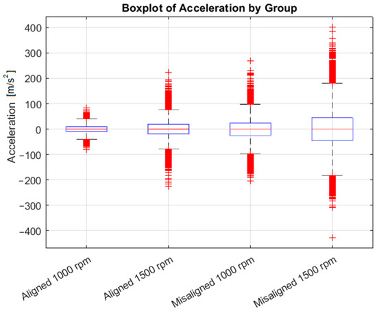
Figure 8.
ANOVA results in the form of a boxplot of acceleration for aligned and misaligned bearings, while functioning at 1000 rpm and 1500 rpm.
From Table 4, it can be interpreted that the differences between the group means are not statistically significant, given the value of 1.44. Also, the sum of squares value for the groups (SS = 4.314) indicates that the variability between the groups is very small compared to the huge variability within the groups (Error SS = 670,400,309.33). This further supports the conclusion that there are no meaningful differences between the group means, meaning there is no significant difference between the groups in terms of the acceleration data. The results suggest that the speed and alignment conditions have little to no effect on the acceleration measurements, based on this particular dataset. To strengthen the generalization and reproducibility of the results, the proposed condition-monitoring method of computing baseline statistical indicators, followed by robust regression analysis, was validated using the publicly available CWRU bearing dataset [17]. Specifically, we utilized four distinct datasets: two sets representing a healthy bearing, of which one was running at 1750 rpm with a load of 2HP, and the other was running at 1730 rpm with a load of 3HP, and two sets of bearings exhibiting an inner race fault, of which one was running at 1750 rpm with a load of 2HP, and the other was running at 1730 rpm, with a load of 3HP. This validation process was undertaken to assess the robustness and generalization of the proposed methodology, ensuring its applicability to real-world scenarios with varying fault conditions. The inclusion of both healthy and faulty bearing data strengthens the reproducibility of the results and provides further empirical evidence of the method’s effectiveness in condition monitoring and fault detection.
The method of analysis proposed within the current paper—namely, the use of statistical indicators, followed by a robust regression model—is validated by the results depicted in Table 5, where it is indicated that the bearing state (normal versus inner race faults) has a statistically significant impact on the acceleration signal (p < 0.001). The positive coefficient associated with the “faulty” condition suggests that defective bearings exhibit significantly higher vibration levels compared to healthy bearings.
Table 5.
Robust regression coefficients for applying the proposed method to the CWRU dataset.
Also, although the RPM coefficient is not significant at the 95% confidence level, the interaction between RPM and alignment is significant, indicating that the effect of rotational speed differs between healthy and defective bearings. Specifically, in the faulty state, increasing RPM is associated with a slight but statistically significant change in vibration amplitude.
The statistical indicators were as follows: RMS = 0.0880 m/s2, skewness = −0.1674, kurtosis = 3.5176 and crest factor = 4.2463.
In addition, to assess the statistical significance of the results, we computed the 95% confidence intervals (CIs) for each coefficient, following the robust linear regression analysis. This step is vital for a more comprehensive evaluation of the relationships between the variables, as CIs provide a range of plausible values for the coefficients, thereby quantifying the uncertainty of the estimates. By incorporating confidence intervals, we enhanced the robustness of our findings, offering a more thorough understanding of the effect sizes and further supporting the conclusion that neither alignment nor speed significantly influences acceleration, considering the analyzed data and experimental setup. The results are visible in Table 6.
Table 6.
Confidence interval values, computed for the robust regression coefficients.
From the results, it can be observed that the 95% confidence interval for the intercept is [−3.3163, 3.2117], which includes zero, suggesting that the baseline value of acceleration is uncertain and could be close to zero. This wide interval indicates a high degree of variability in the intercept estimate. Also, the 95% CI suggests that speed, alignment and their interaction do not significantly influence acceleration in the context of this model. The wide intervals for each term highlight substantial uncertainty, indicating that the effects, if present, are likely very small or non-existent.
The lack of significant influence from misalignment and rotational speed could be attributed to several factors. First, the misalignment tested may have been too mild to induce noticeable changes in vibration, particularly because the bearing was operating within its tolerance limits. Additionally, the narrow speed range (1000 rpm and 1500 rpm) may not have been sufficient to capture nonlinear behaviors or resonance effects, which are often more pronounced at higher or more variable speeds. The results can also be explained by the limited range of operating conditions tested in this study, which might not fully capture the range of dynamics that could be observed in more complex scenarios.
Ultimately, while the findings suggest that, under the tested conditions, neither speed nor alignment significantly affected the acceleration measurements, we caution against broad generalizations. This study serves as an initial exploratory analysis, and future research, with a wider range of experimental conditions, including varying misalignment levels, additional fault scenarios and more extensive speed variations, would be crucial to assess whether these variables have a more pronounced effect under different operating circumstances.
4. Conclusions
Regression analysis is a valuable tool for evaluating the degree of influence of different factors on bearing condition, particularly in predictive maintenance applications. The results of this study suggest that, within the specific conditions of the tested dataset, speed and alignment may have little to no significant effect on the acceleration measurements. This implies that, in this particular scenario, these variables may not serve as strong predictors for fault detection. However, given the limited experimental setup, which includes only two rotational speeds and one level of misalignment, these findings should be viewed as preliminary and not broadly generalizable, and the study may be seen as being limited to the chosen experimental framework and serves as an exploratory analysis. Future research incorporating a wider range of operating conditions might lead to more extensive conclusions. Instead, the vibration signal itself, with its characteristic spikes and impulses, emerges as a suitable informative predictor for faulty bearings, highlighting the usefulness of statistic indicators such as skewness, crest factor or RMS. Still, while this study focused on the analysis of bearing performance using time-domain features, it is acknowledged that these indicators, although useful, may have limitations in capturing more complex fault characteristics. Time-domain features primarily reflect the statistical properties of the vibration signal, which may not always provide sufficient discriminative power for detecting subtle or early-stage faults. Frequency-domain and time-frequency domain features, such as spectral kurtosis, wavelet features, and entropy, are known to provide a more comprehensive analysis by capturing information about signal behavior across different frequencies and time intervals. These features are often more sensitive to transient changes and can enhance fault detection, particularly in more complex or dynamic conditions. As a result, future work could explore the integration of these advanced features to improve diagnostic accuracy. Additionally, a hybrid approach combining both time-domain and frequency-domain features could be considered for a more robust fault analysis on bearing systems and could improve diagnostic accuracy and reliability.
It is also important to acknowledge that the dataset used in this study includes only two rotational speeds and a binary alignment condition (aligned/misaligned). While this simplification allows for a more focused analysis, it limits the extension of the findings to real-world bearing operating conditions, where the bearing could experience a wider range of speeds and more complex alignment scenarios. In real-world applications, bearings are subject to varying operational conditions that may involve continuous changes in speed and potentially more intricate alignment variations. Therefore, future research might consider datasets with a broader range of speeds and alignment conditions, and possibly other factors, such as load and temperature, thus reducing the uncertainty in the generalizability of the findings and providing a more comprehensive understanding of the factors influencing bearing vibration behavior under real-world operational conditions. This would help to enhance the robustness and applicability of the results to real-world scenarios.
In this study, we applied robust linear regression analysis that is particularly beneficial in handling non-normal data distributions, which is common in industrial applications where noise and outliers can significantly impact analysis. This approach allowed for more reliable results compared to traditional regression methods that assume normality in data. However, it is important to note that while robust regression can mitigate the influence of outliers and non-normality, it may not capture subtle effects when the predictor set is limited. The findings suggest that neither alignment nor speed significantly influenced acceleration values in this case, but the methodology’s ability to handle complex data structures could be particularly useful in other scenarios where more complex relationships may exist. Future work should consider exploring alternative features or expanding the predictor set to further evaluate the applicability of robust regression in fault diagnosis under varying operational conditions.
Author Contributions
Conceptualization, R.-M.S.; methodology, R.-M.S., D.V. and R.V.; software, R.-M.S., D.V. and R.V.; validation, R.-M.S.; formal analysis, R.-M.S.; investigation, R.-M.S., D.V. and R.V.; resources, R.V.; data curation, R.-M.S., D.V. and R.V.; writing—original draft preparation, R.-M.S.; writing—review and editing, R.-M.S., D.V. and R.V.; supervision, R.V.; project administration, R.-M.S.; funding acquisition, R.-M.S., D.V. and R.V. All authors have read and agreed to the published version of the manuscript.
Funding
This research received no external funding.
Data Availability Statement
The authors confirm that the data supporting the findings of this study are available within the article.
Conflicts of Interest
The authors declare no conflicts of interest.
Abbreviations
The following abbreviations are used in this manuscript:
| MLR | Multiple Linear Regression |
| HI | Health Indicator |
| RMS | Root Mean Square |
| ECDF | Empirical Cumulative Distribution Function |
| CDF | Theoretical Cumulative Distribution Function |
| EMD | Empirical Mode Decomposition |
| LAD | Least Absolute Deviations |
Appendix A
The first statistical feature, root mean square indicator, was determined in order to measure the overall intensity and magnitude of vibrations in the analyzed bearings, considering the experimental dataset.
For determining kurtosis values for both series, it was used in the following formula [18]:
where E(t) represents the expected values of the quantity t, is the mean of analised series, represents the standard deviation and X will take each value of the set.
When the series observations are , , , …,, the coefficient of kurtosis is expressed as the arithmetic mean of the fourth powers of distances, where the latter are calculated between each observation and its variable mean value, denoted by β:
Derived from the kurtosis indicator, in statistics, there is another measure in the form of excess kurtosis, noted γ, which is used to describe if a sample is flatter or more peaked in nature than the normal distribution and it is calculated with the following formula:
In the context of bearing health, high kurtosis (greater than three) often indicates that there are impulsive events in the acceleration signal. This is typically associated with faults such as pitting, cracks, or spalling on bearing surfaces.
The analysis continued with the calculation of skewness to determine the third moment of the distribution. Because most of the statistical techniques used in mechanical fields assume a normal distribution of data, determining whether a set is positively or negatively skewed is useful for improved results. The coefficient of skewness is determined with the following formula:
where is the third central moment, used to measure skewness asymmetry, and is the variance, defined by the following formula:
The last baseline indicator used to analyze the tested bearings, the crest factor, can give a fast insight into the waveform and the amount of impact that is associated with roller bearing wear. The crest factor can be determined with the following formula [19,20]:
where is the maximum amplitude of the signal and is its RMS value.
References
- Li, C.; Yin, X.; Chen, J.; Yang, H. Bearing Fault Diagnosis Based on Wavelet Transform and Convolutional Neural Network. Open Access Libr. J. 2022, 9, 1–14. [Google Scholar] [CrossRef]
- Li, J.; Wang, H.; Wang, X.; Zhang, Y. Rolling bearing fault diagnosis based on improved adaptive parameterless empirical wavelet transform and sparse denoising. Measurement 2020, 152, 107392. [Google Scholar] [CrossRef]
- Damine, Y.; Bessous, N.; Pusca, R.; Megherbi, A.C.; Romary, R.; Sbaa, S. A New Bearing Fault Detection Strategy Based on Combined Modes Ensemble Empirical Mode Decomposition, KMAD, and an Enhanced Deconvolution Process. Energies 2023, 16, 2604. [Google Scholar] [CrossRef]
- Li, W.; Wang, L.; Lu, P.; Hua, L. Bearing Fault Diagnosis Research Based on Empirical Mode Decomposition and Deep Learning. In Proceedings of the 35th Youth Academic Annual Conference of Chinese Association of Automation (YAC), Zhanjiang, China, 16–18 October 2020; pp. 32–37. [Google Scholar] [CrossRef]
- He, M.; He, D. Deep Learning Based Approach for Bearing Fault Diagnosis. IEEE Trans. Ind. Appl. 2017, 53, 3057–3065. [Google Scholar] [CrossRef]
- Zhang, W.; Li, C.; Peng, G.; Chen, Y.; Zhang, Z. A deep convolutional neural network with new training methods for bearing fault diagnosis under noisy environment and different working load. Mech. Syst. Signal Process. 2018, 100, 439–453. [Google Scholar] [CrossRef]
- Yuan, B.; Lu, L.; Chen, S. Research on Bearing Fault Diagnosis Based on Vibration Signals and Deep Learning Models. Electronics 2025, 14, 2090. [Google Scholar] [CrossRef]
- Wang, Y.; Li, D.; Li, L.; Sun, R.; Wang, S. A novel deep learning framework for rolling bearing fault diagnosis enhancement using VAE-augmented CNN model. Heliyon Sci. 2024, 10, e35407. [Google Scholar] [CrossRef] [PubMed]
- Daoud, J. Multicollinearity and Regression Analysis. J. Phys. Conf. Ser. 2017, 49, 012009. [Google Scholar] [CrossRef]
- Giloni, A.; Simonoff, J.S.; Sengupta, B. Robust weighted LAD regression. Comput. Stat. Data Anal. 2006, 50, 3124–3140. [Google Scholar] [CrossRef]
- Tian, Q.; Wang, H. Predicting Remaining Useful Life of Rolling Bearings Based on Reliable Degradation Indicator and Temporal Convolution Network with the Quantile Regression. Appl. Sci. 2021, 11, 4773. [Google Scholar] [CrossRef]
- Yan, M.; Xie, L.; Muhammad, I.; Yang, X.; Liu, Y. An effective method for remaining useful life estimation of bearings with elbow point detection and adaptive regression models. ISA Trans. 2022, 128, 290–300. [Google Scholar] [CrossRef] [PubMed]
- Wang, S.; Xiang, J.; Zhong, Y.; Zhou, Y. Convolutional neural network-based hidden Markov models for rolling element bearing fault identification. Knowl.-Based Syst. 2018, 144, 65–76. [Google Scholar] [CrossRef]
- Băltoiu, A.; Dumitrescu, B. Bearing Semi-Supervised Anomaly Detection Using Only Normal Data. Appl. Sci. 2025, 15, 10912. [Google Scholar] [CrossRef]
- Chen, Y.; Chen, Q.; Wang, R. Bearing Fault Diagnosis Based on Vibration Envelope Spectral Characteristics. Appl. Sci. 2025, 15, 2240. [Google Scholar] [CrossRef]
- Selvamuthu, D.; Das, D. Introduction to Statistical Methods, Design of Experiments and Statistical Quality Control, 1st ed.; Springer: New Delhi, India, 2018. [Google Scholar]
- Case Western Reserve University. Case School of Engineering. Bearing Data Center. Available online: https://engineering.case.edu/bearingdatacenter/12k-drive-end-bearing-fault-data (accessed on 16 October 2025).
- Johnson, R.; Wichern, D. Applied Multivariate Statistical Analysis, 6th ed.; Pearson: Upper Saddle River, NJ, USA, 2007. [Google Scholar]
- Martinez, W.L.; Martinez, A.R. Computational Statistics Handbook with MATLAB; Chapman&Hall/CRC: Boca Raton, FL, USA, 2002. [Google Scholar]
- Althoff, H.; Eberhardt, M.; Geinitz, S.; Linder, C. Advances in Crest Factor Minimization for Wide-Bandwidth Multi-Sine Signals with Non-Flat Amplitude Spectra. Comput. Sci. Math. Forum 2022, 2, 11. [Google Scholar] [CrossRef]


Disclaimer/Publisher’s Note: The statements, opinions and data contained in all publications are solely those of the individual author(s) and contributor(s) and not of MDPI and/or the editor(s). MDPI and/or the editor(s) disclaim responsibility for any injury to people or property resulting from any ideas, methods, instructions or products referred to in the content. |
© 2025 by the authors. Licensee MDPI, Basel, Switzerland. This article is an open access article distributed under the terms and conditions of the Creative Commons Attribution (CC BY) license (https://creativecommons.org/licenses/by/4.0/).