Abstract
This work addresses the challenges of airline planning, which requires the integration of flight scheduling, aircraft availability, and maintenance to ensure both airworthiness and profitability. Current solutions, often developed by human experts, are susceptible to bias and may yield suboptimal results due to the inherent complexity of the problem. Furthermore, existing state-of-the-art approaches often inadequately address critical factors, such as maintenance, variable flight numbers, discrete time slots, and potential flight repetition. This paper presents a novel approach to aircraft routing optimization using a model that incorporates critical constraints, including path connectivity, flight duration, maintenance requirements, turnaround times, and closed routes. The proposed solution employs a simulated annealing algorithm enhanced with specialized perturbation operators and constraint-handling techniques. The main contributions are twofold: the development of an optimization model tailored to small airlines and the design of operators capable of efficiently solving large-scale, realistic scenarios. The method is validated using established benchmarks from the literature and a real case study from a Mexican commercial airline, demonstrating its ability to generate feasible and competitive routing configurations.
1. Introduction
Airline operations management involves several planning problems. This work focuses on the Operational Aircraft Maintenance Routing Problem (OAMRP), which builds aircraft routes that meet maintenance requirements. Regulations mandate maintenance after a predetermined number of flight hours. This paper considers the most frequent preventive maintenance checks, i.e., the A-check [1].
The OAMRP requires creating a route for each aircraft under the following constraints: every flight is covered only once, a minimum turn time of one hour exists between consecutive flights, the total flying time since the last maintenance check must not exceed the maximum allowed, and maintenance checks must be completed at authorized facilities, grounding the aircraft for the minimum required time.
Table 1 and Table 2 summarize optimization procedures and model formulations for the OAMRP, respectively. Table 1 details the algorithms, objectives, and maintenance constraints used in the literature.
Early work (pre-2006) established foundational models such as the Flight Segment Model (FSM) [2] and the Euler Tour, with later contributions introducing connection networks [3] and daily planning with flying hour limits [4]. This period was characterized by exact methods.
The second period (2011–2018) saw methodological expansion. Contributions included time–space networks [5], reformulation–linearization techniques [6], multi-commodity flow models solved with heuristics [7], and large-scale neighborhood search [8]. This era introduced heuristic algorithms to solve larger real-life networks efficiently [5,7,9,10]. Metaheuristics such as ACO, SA, and GA were applied to the hard problem of NP [9], and the models began to incorporate more operational constraints (M1–M5) [6,8,11].
Recent work (2019–present) continues to integrate additional operational constraints, such as workforce capacity (M4) and maintenance station working hours (M5), often treated as feasible route constraints (M6). The solutions employ advanced techniques such as multi-objective MILP [12], reinforcement learning [13], hybrid algorithms [14,15], and CPLEX-heuristic combinations [16].
This review identifies remaining challenges: most linearization and hybrid approaches actually perform several simplifications; for instance, assigning a predefined number of flight slots for continuous departure and arrival times, predefined maintenance slots and predefined number of flight repetitions (usually each flight is assigned only once), as well as rotation periods of one of three days, while the realistic case is a week. These changes make the problem unrealistic and increase its complexity, typically by increasing the number of variables. In the real world, the number of time slots is not known until the route is optimized. Additionally, predefined departure and arrival times can be assigned in advance according to infrastructure availability; therefore, departure times are usually discrete and cannot be assigned continuously. Recent literature on drones and urban air mobility [17,18,19,20,21] typically omits maintenance constraints.
This work addresses the Operational Aircraft Maintenance Routing Problem (OAMRP), which involves constructing aircraft routes that comply with maintenance regulations, such as mandatory A-checks after a predetermined number of flight hours [1]. The problem is constrained by route continuity, minimum turnaround times, maximum flight hours between maintenance checks, and the requirement that maintenance be performed in authorized facilities. The main contributions of this paper are a compact graph-based optimization model for OAMRP and novel perturbation operators designed for an efficient metaheuristic solution approach. The model utilizes a variable-size representation that determines the number of maintenance slots and flight repetitions as outcomes of the optimization process, employing discrete time slots to improve operational realism.
The development of a model that integrates an increasing number of flights with realistic operational requirements is highly valuable for airline companies, as it enhances practical applicability. Classical approaches often address this complexity by fixing departure and arrival times and generating feasible routes for predefined schedules. In contrast, recent heuristic and metaheuristic methods offer an improved balance between solution feasibility and computational cost. However, many contemporary routing formulations, particularly in emerging applications such as urban air mobility, omit essential maintenance constraints and lack validation with realistic data.
The proposed perturbation operators are designed to efficiently handle large-scale instances. Computational experiments on benchmark problems with up to 16 destinations demonstrate that the method performs competitively and consistently outperforms recent approaches in the literature. Furthermore, the solution framework supports objective functions that maximize time or flight count as proxies for profit, and its modular design allows operators to be integrated into other heuristic frameworks, including those for vehicle routing problems that currently lack maintenance considerations.
In contrast to mixed-integer linear programming (MILP) formulations, such as those presented in [22] for the vehicle routing problem (VRP), our approach highlights several key differences. First, the number of visits to airports (analogous to customers in the VRP) is not fixed; the route can increase or decrease arbitrarily, and a single airport can be visited n times if doing so maximizes the objective function. Additionally, we do not consider the vehicle’s volume capacity. Another important distinction is that flights cannot depart at any time (continuous time variable) but only within predefined slots that depend on both the departure and arrival airports. These characteristics make it challenging to model the problem as a MILP, where continuous time and customer demands play a central role. It is worth noting that airport demand can still be incorporated into a profit-maximization objective function. Moreover, most metaheuristics developed for the VRP or TSP [23,24] employ similar perturbation operators, typically assuming a fixed-size route (i.e., a predefined number of airports to visit) and restricting the number of visits to each airport, usually one or two. Similar to MILP-based approaches, these metaheuristics generally ignore discrete departure times between consecutive airports. Finally, both MILP and metaheuristic methods neglect maintenance constraints, such as those requiring aircraft to visit designated AM maintenance airports to perform mandatory MaxNMtto maintenance services. To the best of our knowledge, this is the first work to incorporate such a realistic constraint. Other recent studies [25,26] have addressed stochastic (non-scheduled) maintenance services, which are realistic but not typical or desirable in practical aircraft routing. Finally, it is worth emphasizing that integrating a profit-maximization objective or adding penalties for a minimum number of visits to specific airports is straightforward in our approach: only the objective function must be modified, while the rest of the algorithm remains unchanged. This is not the case for MILP or metaheuristic methods for VRP or TSP, where incorporating discrete departure schedules and maintenance slots requires significant additional modeling or analytical effort.

Table 1.
Characteristics of optimization procedures for solving the OAMR problem.
Table 1.
Characteristics of optimization procedures for solving the OAMR problem.
| Reference | Optimizer | Objective | Constraints |
|---|---|---|---|
| [2] | Branch and price | Min total cost | – |
| [27] | Polynomial-time algorithm | Find feasible routes | – |
| [3] | Deep first and random search | Min maintenance and reassignment cost | M1, M4 |
| [4] | Branch and price | Min number of unused legal flying hours | M2, M4 |
| [5] | CPLEX 10.0 | Min connection and maintenance costs | – |
| [6] | CPLEX 12.1 | Find feasible routes | M1, M2, M3 |
| [7] | Branch and bound, compressed annealing | Max utilization of remaining flying time | – |
| [8] | Large-scale neighborhood search algorithm | Min the sum of remaining flying time | M1, M2, M3 |
| [9] | ACO, GA, SA | Max the through value | M1, M4 |
| [10] | Branch and bound | Min the number of maintenance misalignments | M1, M2, M4 |
| [11] | CPLEX 12.1 | Max total profit | M1, M2, M3, M4, M5 |
| [12] | Heuristic | Min maintenance violations and not airworthy aircraft | M2, M3, M4 |
| [13] | Reinforcement learning vs CPLEX | Max through value of the route | M2, M3, M4 |
| [14] | Hybrid Gasimov’s and ACO | Max the total profit through value of the route | M6 |
| [16] | CPLEX-Heuristic | Max the number of cyclic routes | M1, M6 |
| [15] | Hybrid IACO-CPLEX | Min the sum of aircraft usage, idle time, and fuel-burn related costs | M1, M2, M3, M4 |
M1: Each aircraft must undergo one maintenance check for every n days. M2: The total flying hours of each aircraft between two consecutive maintenance checks must not go beyond the maximum allowable flying hour limit. M3: The total number of take-offs of each aircraft must not go beyond the allowed maximum number of take-offs. M4: The number of aircraft to be maintained at each maintenance station should not exceed the available workforce capacity. M5: Aircraft maintenance checks should be attended within the working hours of the maintenance stations. M6: Feasible route constraints.
Table 2.
Issues of the formulations for the OAMR problem solution.
Table 2.
Issues of the formulations for the OAMR problem solution.
| Reference | Mtto. Type | Planning | Network | Model | Data |
|---|---|---|---|---|---|
| [2] | – | Weekly | Connection network | FSM RTNOM | G |
| [27] | A | 3–4 days | Network flow problem | Euler Tour | – |
| [3] | A, B | Weekly | Connection network | MCNF | – |
| [4] | A, B | Daily | Set partitioning | – | – |
| [5] | Night-Transit | Daily | Time–space network | MIP RTNOM | RL US Carrier |
| [6] | A | Daily | Connection network | NAFF | RL (United airlines) |
| [7] | – | Weekly | Connection network | MCNF | RL |
| [8] | A | Weekly | Connection network | MCFP | – |
| [9] | – | 4 days | Connection network | MIP | – |
| [10] | MWD | Weekly | Connection network | – | RL Canadian |
| [11] | A | 4 days | Modified connection network | – | EgyptAir |
| [12] | C | 30 days | – | MMILP | Flightradar24 |
| [13] | A | 4 days | Network flow based/Markov decision process | NAFF | – |
| [14] | A | Daily | Connection network | ATSP | – |
| [16] | A | 3 days | Connection network | ATSP | RL (Florida Express) |
| [15] | A | 4 days | Connection network | – | BTS |
FSM: Flight Segment Model. RTNOM: Rotation Tour Network Optimization Model. MCNF: Multi-Commodity Network Flow. MIP: Mixed Integer Programming. MCFP: Multi-Commodity Flow Problem. MMILP: Multi-objective Mixed Integer Linear Programming. NAFF: Node Arc Flow Formulation. MWD: Maintenance Workload Due. ATSP: Asymmetric Travelling Salesman Problem.
2. Methodology
This proposal generates a flight schedule for an aircraft, referred to as a rotation R, within a specified time frame. Hence, the desired rotation is a sequence of flights that repeats cyclically over a defined period, optimized by maximizing the number of flights or the flight time.
2.1. Solution Representation
Firstly, we define a set of parameters used to evaluate the solution’s performance. Given a set of destination airports D, as shown in Equation (1), a rotation R consists of a sequence of these airports and the corresponding departure times. However, airports are often not fully connected; that is, not every airport has a direct flight to every other airport. The connecting flights are represented as ordered pairs (origin, destination), stored in a matrix E (Equation (2)). The row indices in E correspond to those in the schedule matrix H (Equation (3)) and the flight duration matrix T (Equation (4)). For instance, if a connection is in row p, the available departure times are in row p of H; if the selected time is , the duration is in the same position of T. The rotation is subject to a fixed period (Equation (5)). A valid solution must schedule all flights within , after which the same sequence repeats. The turnaround time s (Equation (6)), the maintenance airports (Equation (7)), and the maintenance time (Equation (8)) allow for calculation of the complete rotation considering the times when the aircraft will be on the ground and where its maintenance will be performed.
2.2. Parameters to Define a Rotation (Input Data)
Destination set: set of destination airports.
Set of possible connecting flights: the connecting flights are organized as ordered pairs (origin, destination), stored in a matrix E with rows and two columns: the first column lists the origins, and the second column lists the destinations. is the total number of different connecting flights.
Departure times of flights in E: the indices of the rows in matrix E are the same as those in the schedule matrix H.
Flight time: flight duration.
Rotation period: the rotation is subject to a fixed period which includes both flying and rest times. It is denoted by
Turnaround time: the minimum time required between consecutive flights. It is denoted by
Maintenance airports: maintenance airports are stored as an array with the numeric label of the destination airport that serves as a maintenance base.
Maintenance time: the time to perform aircraft maintenance.
Method output: rotations are the outputs of the method introduced in this article, and these are represented in two ways:
- A matrix R, as seen in Equation (9), is a matrix with rows (number of flights), such that the first column, with elements , represents the airports of origin, the first index , indicates a row in the connection matrix E, while the second, 1, indicates that this entry comes from the first column of the matrix E. The second, with elements , is the destination airport; this entry comes from the second column of the matrix E to ensure a real flight connection. For the third column with elements , the first index is the same as the previous elements; that is, refers to the same row index in the E, H, and T matrices. The second index, j, is a column in H that indicates a selected departure time for the corresponding flight. In addition, the flight duration is found in matrix T at position . This representation is suitable for direct human interpretation, but it does not facilitate compact storage and the application of perturbation operators, which are commonly used in most direct search algorithms.
- Matrix X in Equation (10) is a second representation of a rotation. This representation facilitates compact storage and the application of perturbation operators. It has a number of lines ; therefore, the number of rows is the same as that of R. Nevertheless, this representation assumes that the entry is the origin airport while is the destination, and so on. In general, is the origin airport for , and is the destination for . Finally, the last origin airport is , and the last destination airport is . This representation assumes the fulfillment of two constraints: firstly, a destination airport becomes the next origin airport; this is the path constraint, which ensures that connecting flights are possible. Secondly, the last destination airport is the first origin airport; this is the closed path constraint, which ensures that the rotation is repeated cyclically. Nevertheless, these constraints seem obvious; a method for generating and perturbing candidate solutions must ensure that both are fulfilled.
2.3. Objective Functions
Objective functions measure the performance of a candidate solution; that is, they are used to determine whether one rotation is better than another. Objective functions are used alternately for mono-objective maximization; the actual selection of one of them depends on the decision-maker.
- Maximization of flight duration: It assumes that increasing the flight time increases the profit, measures the sum of flight durations of the rotation, using the data from matrix T in Equation (4) and the indexes of rotation in Equation (9), as shown in Equation (11).If available, profit data can be incorporated by substituting the time variable with the profit variable in Equation (11). This substitution does not require substantial alteration to the underlying method.
- Maximization of the number of flights: It assumes that maximizing the number of flights in the rotation increases the profit. This number of flights is the number of rows of rotation, as shown in Equation (12).
2.4. Constraints
A feasible candidate solution must fulfill the following constraints to ensure a physically possible rotation:
- Path constraint: In rotation R, the flight from for always departs from the previous airport so that . In a mathematical sense, it means that the sequence of visited vertices forms a walk or path. For example, Figure 1 shows that the sequence of visiting nodes is . All connections must exist in the matrix E. For example, the table in Figure 1 illustrates the rotation in the figure; the second and third columns denote the departure and arrival airports, respectively. The right airport is the left airport of the row below. The departure time is in the third column; if the departure time of a flight is earlier than the previous, the departure day in the fourth column is computed to fulfill this constraint.
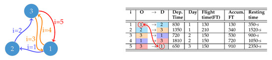 Figure 1. Rotation example. Colors in the O→D column represent a destination that is the origin of the next flight. The arrow indicate the the initial and final airports are the same. The resting time is the gap between flights minus the turnaround s.
 - Duration constraint: A rotation R is a sequence of flights that repeat every certain number of days. Therefore, the total rotation time must not exceed the period . Note that the rotation duration time is not only the flight time and turnarounds, but also the downtime due to schedule limitations. For example, if a flight arrives at 12:00 p.m. and departs at 11:00 a.m., a full day must pass before departs. In Figure 1, assuming a of 3 days, the relative day of each flight is shown in the Day column, which is assigned automatically by an algorithm to ensure that they do not overlap. Assuming a turnaround time of min, the total rotation time is calculated using the departure time of the first flight (8:30, recorded as 830 in the Dep. time column) on the first day and the arrival time plus turnaround of the last flight. The last flight departs at 6:50 on the third day (row 5, columns 3 and 4), flies for 1 h and 50 min, arrives at 8:40, and undergoes a 40-min turnaround. Thus, the operation ends at 9:20 on the third day. Then, the aircraft rests by 23:50 h minus 40 min, as shown in the Resting time column—that is, 23 h and 10 min—to restart the rotation for the next day (first day again) at 8:30.
- Closed-path constraint: A closed path is one that ends at the vertex at which it started. In our case, it means that the sequence of flights ended at the airport where it started, which is necessary for rotation R to repeat exactly the same flights every time interval . In Figure 1, it is shown with a red arrow from the last destination airport to the first origin airport.
- Constraint of turnaround: The turnaround time s is a minimal gap between landing and taking off. In Figure 1, the last column subtracts the turnaround time from the difference between arrival and the next departure; this value must always be positive to ensure that flights do not overlap.
- Number of maintenance services constraint: The number of maintenance opportunities that are possible within a rotation R is computed by counting the gaps between arrivals and next lading minus the turnaround time that are greater than or equal to the maintenance time. For example, assuming h (800 in our notation) and a turnaround time of min, in Figure 1, the number of maintenance opportunities is the number of resting times that are lesser or equal to 800; in this case there are 4, and only the first flight has a resting time of 3:10 h. Hence, if the number of maintenance opportunities is equal to or lower than the number of maintenance services, the rotation is feasible.
A feasible rotation fulfills the constraints of path, duration, turnaround, closed path, and number of maintenance services.
2.5. Candidate Solution Evaluation and Constraint Management
The proposed evaluation algorithm manages the constraints as follows:
- The path constraint presents two cases: The first case involves proposing the initial random rotation. The first flight is selected from the total possible flights in matrix E. Then, the next flight is randomly selected from the subset of flights that fulfill the constraint (i.e., flights connected to the previous one). The second case is a perturbation, where a block of connecting flights is replaced by another. The algorithm ensures that the block of flights inserted fulfills the path constraint. If no feasible solution is found after several trials (specifically, 30 trials in our implementation), the solution is not perturbed and is returned in its current form.
- For managing the duration constraint, the algorithm computes the total rotation time; if it is greater than the rotation period, then the candidate solution is penalized. The penalization method guarantees that a feasible solution has a better objective function value than an unfeasible one. Let be the total rotation time, be the rotation period, and be the flight time; hence, the penalization for this objective is shown in Equation (13). Notice that for a feasible solution, is always greater than because , and an unfeasible solution is always less than .In the same regard, assuming that a rotation X has at least 2 rows (1 flight), Equation (14) is greater than for a feasible solution and less than for an unfeasible one.
- The closed-path constraint is managed by removing flights from the rotation until the last flight is connected to the first.
- The turnaround constraint is managed by verifying that there is a lapse time s between a flight and the next, or assigning the flight to the next day.
- The number of maintenance services constraint is managed by inserting a maintenance service each time a maintenance airport is visited until the number of desired services is fulfilled. Inserting the maintenance services very possibly increases the duration time; hence, the penalization is applied to the duration time.
2.6. Simulated Annealing
The optimal rotation is the solution to a combinatorial problem; hence, there are no efficient algorithms that guarantee its discovery. On the other hand, direct-search algorithms for global optimization, such as simulated annealing (SA), have consistently yielded successful results in solving this type of problem [28,29]. Simulated annealing [30] is a search method that evolves a solution using perturbations to generate new neighboring solutions and replaces the current solution according to an acceptance criterion. This algorithm, proposed in 1983 by Kirkpatrick [31], is based on principles from thermodynamics and the annealing process in steel manufacturing. In this process, a solid is heated to a liquid state and then gradually cooled to form a crystalline structure. There are many algorithms based on stochastic perturbations, such as the family of evolutionary algorithms and swarm intelligence; nevertheless, SA is possibly the most widely used and tested. Furthermore, SA is well-suited for handling problems of varying sizes without requiring significant modifications. For instance, new problem requirements are straight-forward incorporated as constraints and handled by adjusting perturbation procedures without altering the overall algorithm. SA in Algorithm 1 is particularly notable for being a probabilistic method that prevents the stagnation that often occurs in other algorithms. The SA algorithm is presented in Algorithm 1. The search process explores neighboring solutions using perturbations. It initially exhibits a high degree of variance, but this variance decreases as the algorithm progresses. This allows the algorithm to explore a wide range of solutions. The elements that integrate the SA algorithm, as described in Algorithm 1, are the following:
- An initial candidate solution: , which is generated randomly.
- A perturbation, , functions to generate candidate solutions in the neighborhood of another.
- A test solution from the perturbation of the initial solution in a neighborhood: .
- The objective function: .
- Number of steps before recalculating the neighborhood: .
- Number of steps before updating the temperatures: .
- The annealing parameter: to reduce the temperature.
- Maximum number of (while) loops without improving the best solution as a stopping criterion.
Recall that the perturbations, applied to the rotations R, use the representation of two columns, as shown in Equation (10).
Lines 1 to 6 are initializations and initial solutions. The infinity initial temperature means that the first iterations are completely exploratory, as the perturbed solution is always accepted with this value. These iterations also serve to estimate an adequate initial temperature, independently of the objective function, as the estimator of the mean of the objective function. The algorithm begins with an initial candidate solution, , and a test solution, . This test solution is evaluated using an energy function to calculate the acceptance probability, and the Metropolis algorithm determines whether this new configuration is accepted. The stopping criteria are 5 repetitions of the best objective function at the while-level cycle, or the average probability of acceptance of the perturbation in the last while-cycle. The remaining algorithm is the standard SA. Line 11 perturbs the current solution. In line 14, the best solution is updated if necessary, as shown in line 18. This evaluation determines whether to accept a neighbor with a lower energy or one with a higher energy based on a probability that depends on the temperature T, as shown on line 17.
The main contributions of this work are the optimization model, the perturbation methods used to propose candidate solutions, and the constraint handling procedures.
| Algorithm 1 Simulated Annealing |
Require: ▷ Initial temperature (high initially). ▷ Annealing factor. ▷ Perturbation function. ▷ Objective function. ▷ Converts the problem to minimization. ▷ Iteration counter. ▷ Initial rotation ▷ Initialize best solution ▷ Evaluation ▷ Best OF initialization; while Until the stop criterion is met do for do for do if then end if if ( then else if then end if end for if then end if end for ; Update and end while |
According to Algorithm 1, the maximum computational complexity is O(|T| NTNsNR3). |T| is the number of temperature reductions, NT and Ns are algorithm parameters (taken from the original Corana’s SA), NR stands for the maximum number of flights in the rotation, corresponding to the most inner loop in Algorithm 1 (NR operations). Since perturbations require up to NR operations, and the same applies to solution repairing, the total number of operations is the multiplication of three NR.
Notice that NR is bounded by the minimum flight time, min(T), over the rotation time minus the maintenance time times the number of maintenance services, integer(min(T)/(ΔT -(MaxNMtto)(MT))). Nevertheless, this bound is usually far from the actual value, but it serves to show a complexity bound in the worst case. Furthermore, the relevant issue is that the time complexity strongly depends on the rotation length, which in turn mainly depends on the rotation period and the flight times.
2.7. Perturbation Operators
The SA, in Line 9 of Algorithm 1, utilizes perturbation operators; these operators generate new neighboring candidate solutions to the current working solution , modifying or changing flights or schedules. Recall that the X representation is actually a matrix of airports, in the first column, and schedules (departure times) in the second. For all flight perturbations, the first and last airports remain unchanged.
- Perturbation 1 (PERT-1): Airport substitutionA randomly chosen index denoted by , corresponding to an airport, is selected and replaced by a random airport from those with a connection with the previous airport at position . Then, it is verified that a connection to the subsequent airport, , exists. Finally, a random schedule is selected for the flights, which is straightforward by selecting a non-empty position in the H matrix, corresponding to the rows for the flights. If the new airport, chosen at random, is the same as the existing one or has no additional flights compared to the current, we repeat the random selection process. Table 3 presents an example of this flight perturbation. The selected airport is that in row 3 (); hence, airport 4 is randomly replaced by airport 3. Then, it is verified that such connection flights exist, specifically 2-3 and 3-1, and new schedules are selected for these flights. The changes are in red.
Table 3. PERT-1: Perturbation of random substitution of one airport and the schedules of the two newly generated flights. In this example, airport 4 is substituted by 3 (marked in red). Background colors emphasize that the destination of the previous flight is the origin of the current one, as well as airport repetitions. Arrows indicate airport connections, and red font denotes changes introduced by the perturbation.
- Perturbation 2 (PERT-2): Schedule substitutionIn this perturbation, a random airport position is selected, and a new random departure time for the flight from the airport at position to the airport in position is selected. In this case, the first and last airports can be selected.In Table 4, two flights are observed where airport 4 is selected randomly and is connected to airport 5; thus, a new schedule of 1535 (15:35) is assigned, and the two resting times are recomputed.
Table 4. PERT-2: Schedule substitution. The departure time of flight 4 is changed, which affects the resting time of the two flights. Background colors emphasize that the destination of the previous flight is the origin of the current one, as well as airport repetitions. Arrows indicate airport connections, and red font denotes changes introduced by the perturbation.
- Perturbation 3 (PERT-3): Multiple flight deletion and one flight additionIn this perturbation, two positions of the airport column are selected at random, with the beginning and end . The airports between and are removed. Then, we search for new airport connections between and and select one of them at random. If it is not possible to find a connection flight, the process is repeated a maximum of 15 times; otherwise, the rotation is returned as is.Table 5 shows an example of the perturbation. The gray positions from 1 to 4 are selected, both positions have airport 1 in the airport column, then airports 2 and 4 are removed, and airport 2 is inserted, generating the connection flights from 1 to 2 and 2 to 1, marked in red in the second table.
Table 5. PERT-3: Indices 1 and 4 are chosen at random, then the intermediate rows, 2 and 3, are deleted in the upper table, and airport 2 is inserted in the second table. This generates the flights in rows 2 and 3, and the new schedules are assigned at random. Background colors emphasize that the destination of the previous flight is the origin of the current one, as well as airport repetitions. Arrows indicate airport connections, and red font denotes changes introduced by the perturbation.
- Perturbation 4 (PERT-4): Combination of PERT-3 and PERT-1Perturbations 3 and 1 are combined by applying them sequentially.
- Perturbation PERT-5: Schedule shiftingThis perturbation operates similarly to the schedule substitution method (PERT-2), with the difference that the departure schedule of a randomly selected flight is changed with a probability of 0.2 to the next available schedule and with a probability of 0.8 to the previous one. The schedules are considered cyclic, meaning that the next schedule after the last one is the first in the sequence.Recall that flights are scheduled sequentially within the same day if the departure time allows; otherwise, the flight is assigned to the next day. The main purpose of this perturbation is to increase the number of flights accommodated within the rotation period. Since departure times are sorted in increasing order, shifting a flight to an earlier or later schedule can improve the overall fit within the rotation period. An example of this perturbation is shown in Table 6, where the affected schedule is highlighted in red. The selected flight in row 4 is moved forward from 1200 to 1915. As a result, the rest time between flights is adjusted, as indicated in the last column.
Table 6. PERT-5: A departure schedule from row 4 is shifted to the next departure time, from 1200 to 1915. Background colors emphasize that the destination of the previous flight is the origin of the current one, as well as airport repetitions. Arrows indicate airport connections, and red font denotes changes introduced by the perturbation.
- Perturbation 6 (PERT-6): Random perturbation or addition of two connection airportsThis perturbation consists of a random selection of the previous perturbations and a new drastic perturbation for adding flights. Considering that adding flights leads to large unfeasible rotations, the previous perturbations alleviate these problems selected at random: PERT-3 is applied with a probability of 0.09, PERT-1 with a probability of 0.18, and PERT-2 with a probability of 0.18, PERT-4 with a probability of 0.45, and finally, with probability of 0.1, the addition of two connection airports is applied as follows: a random index, , is randomly selected from the rotation X (i.e., the index of an airport in the sequence representation X). The previous index is denoted as . Then, we search for the set of airports, denoted by , that has a flight originating from . For each airport in , we look for flights from to such that is the origin of a flight that arrives at . Then, the pair of airports (,) is added to an array of possible flight additions. A pair of airports (,) is randomly selected from the array and added to the rotation X after . Hence, this perturbation adds two airports to the rotation in the X representation and 3 flights in the R representation: from to , from to , and from to . The corresponding flight schedules are assigned randomly. This process is repeated until a successful perturbation is achieved or a maximum of 15 attempts is reached.An example of this perturbation is shown in Table 7, where the search path for the two new flights that are added to the rotation R is observed; as can be seen in the final rotation of Table 7, there is an increase from six to eight flights in the new rotation R.
Table 7. PERT-6 applies one of the previous perturbation operators with different probabilities; otherwise, it adds two airports—in this case, airports 3 and 4, marked in red—the departure times are selected randomly, and the perturbation guarantees the path constraint. Background colors emphasize that the destination of the previous flight is the origin of the current one, as well as airport repetitions. Arrows indicate airport connections, and red font denotes changes introduced by the perturbation.This perturbation consists of a random selection from the previously defined perturbations, along with a new, more drastic perturbation aimed at adding flights. Since adding flights can result in large, infeasible rotations, the previous perturbations are used to help mitigate these issues. The selection is made randomly as follows: PERT-3 is applied with a probability of 0.09, PERT-1 with 0.18, PERT-2 with 0.18, PERT-4 with 0.45, and with a probability of 0.10, the new flight-addition perturbation is applied.In this new perturbation, a random index is selected from the rotation X (i.e., the index of an airport in the sequence representation X). The preceding index is denoted as . We then identify the set of airports that have outgoing flights from . For each airport , we look for flights from to another airport such that is the origin of a flight arriving at . Each valid pair of airports is added to an array of possible flight additions.A pair is then randomly selected from this array and inserted into rotation X immediately after . As a result, this perturbation adds two airports to the rotation in the X representation, and three flights replace one in the R representation: from to , from to , and from to . The corresponding flight schedules are assigned randomly. This process is repeated until a successful perturbation is achieved or a maximum of 15 attempts is reached.
2.8. Rotation Repairing
The initial candidate solution is randomly generated; hence, there are cases where a rotation does not fulfill the path constraint. Then, a repairing method is applied as follows:
- Remove the last flight. For example, Figure 2 shows a rotation with airport 2 as the last destination and airport 1 as the first origin; hence, there is no closed path. Removing the last flight, in row 6 of the first table, going from airport 1 to 2 alleviates the problem, as noted in row 5 of the second table and in the market with in the graph; the first origin and last destination of the repaired rotation are airport 1.
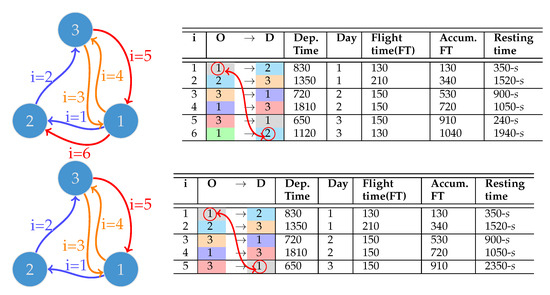 Figure 2. Repairing a rotation for fulfilling the closed path constraint. The first repairing attempt is simply to remove the last flight. Circles indicate the initial and final airports, which must be the same, and how the repair procedure makes the rotation feasible.
 - There are cases that are not repaired by the previous strategy. For example, in Figure 3, in the first table, the flight in row 6 from airport 2 to 3 is removed; nevertheless, the last airport in the modified rotation is 2, so the closed path constraint is not fulfilled. Hence, a second repair step is to look for a flight from the current last origin, that is, airport 3 (since a row has been removed), to the first origin, that is, airport 1. This results in the rotation in the second table and graph, which fulfills the closed path constraint.
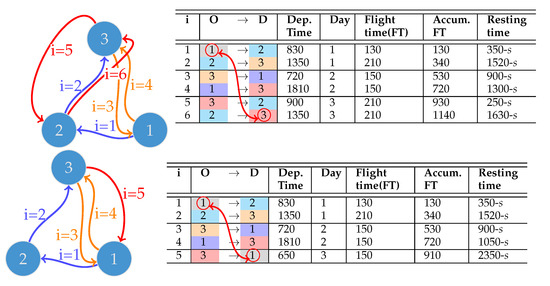 Figure 3. Second repair of a rotation to fulfill the closed path constraint. Firstly, the last flight is removed (row 6 of the first table, from 2 to 3), as the rotation remains unfeasible, then we look for a flight from the last destination (airport 3) to the first origin (airport 1). Circles indicate the initial and final airports, which must be the same, and how the repair procedure makes the rotation feasible.
 - Finally, if neither removing a flight nor looking for connecting flights makes the rotation feasible, the process is repeated.
Finally, a modification is made that considers the idea that in some rotations, a certain amount of maintenance may not be available; therefore, forced maintenance (MF) is introduced, which must comply with a minimum amount of maintenance within the assigned time period.
The amount of maintenance to be performed in a rotation is entered in the input data through the variable MaxNMtto. After a rotation is disturbed, the flight times are calculated, including the accumulated time of rotation R and the forced maintenance. Specifically, while the accumulated time is being calculated, it is verified which destinations it is visiting. If it passes through the maintenance airport and up to now no maintenance has been performed, then a maintenance operation is scheduled. In this case, the duration of the flight from where it arrives to the maintenance base, the turnaround time s, and the maintenance time are considered. Then, the amount of maintenance time it will require from when it arrives at the maintenance base until the next flight begins is calculated. If it is not possible to enter the forced maintenance on a certain day due to time constraints, it is rescheduled for the next day.
The final result of the rotation indicates the number of maintenance opportunities available during the rotation, the timing of maintenance, and the amount of time allocated for maintenance.
3. Results
Three experiments are conducted to evaluate the algorithm’s performance. The first is a pilot experiment designed to demonstrate the algorithm’s ability to generate solutions comparable to those produced by a human. This experiment serves as a baseline validation of the algorithm using the objective function of maximizing flight time.
The second and third experiments involve larger-scale scenarios in which finding solutions is more challenging due to the increased volume of data. In these experiments, both objective functions, maximizing flight time and maximizing the number of flights, are tested. These scenarios assess the algorithm’s ability to identify feasible solutions under more complex conditions.
The key difference between the second and third experiments is the implementation of forced maintenance. It is not applied in the second experiment, but it is included in the third. The code for reproducing the results of these experiments, along with the corresponding input data, is provided in [32].
3.1. Study Case 1: Data from Bazargan Book
For this first case, the example presented in the book Airline Operations and Scheduling [33] is taken as a reference, based on the American Airline Ultimate Air that carried out domestic flights within the United States in the cities of New York (JFK), Boston (BOS), Los Angeles (LAX), San Francisco (SFO), Miami (MIA), Atlanta (ATL), Washington D.C. (IAD), and Chicago (ORD). This first test is used to verify that the algorithm works correctly, that is, it complies with established restrictions and maximizes the objective function. Therefore, the execution uses the most general perturbation, PERT-6. In this case, the rotation period is = 3 days, with a turnaround time s of 45 min. The New York (JFK) airport is the maintenance base, with a TMLA maintenance time of 8 h; it is not required to force maintenance, that is, MaxNMtto is set to 0. The parameters used in the algorithm are as follows:
- Ns: 5
- Nt: 5
- MaxfCount: 5
- rT: 0.95
The input data is presented in Table 8. There are six possible airports, with three or four departure times for each airport. Notice that the flight time, in this case, is symmetric, that is to say, the time from LAX to JFK is the same as that from JFK to LAX. Nevertheless, this is not necessary for our proposal.
Table 8.
Input data for study case 1. NA stands for “Not Available” and indicates that there are no additional departure slots.
Results for Study Case 1
We execute the proposed algorithm 15 times; the flight time for each is shown in Figure 4. The minimum (worst) flight time is 28.5 h, the maximum (best) flight time is 37.5 h, the mean is 31.13 h, the median is 30.5 h, and the standard deviation is 2.27 h. All executions deliver feasible solutions. Table 9 and Figure 5 show the best solution. Notice that there are no constraints or terms in the objective function that require including many destinations, and hence the algorithm uses the flights with the maximum flight time.
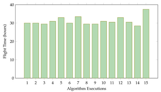
Figure 4.
Objective function values of the best solution found in 15 independent executions of the SA for the flight time maximization problem using the data for study case 1.
Table 9.
Best solution found in 15 executions of the proposal for flight time maximization for study case 1.
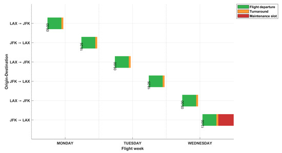
Figure 5.
Representation of the rotation for the best flight time of study case 1.
3.2. Study Case 2: Data from a Mexican Airline
To evaluate the performance of the algorithm with different perturbations and objective functions in a real-world case, public data [34] from a Mexican airline is used. This data includes a historical record of the company’s flight operations over several years. For this test, the dataset corresponds to the period from 9 January to 15 January 2023. The simulation parameters include a turnaround time of 30 min and an 8-hour TMLA maintenance duration. Mexico City (MEX) is designated as the maintenance base, as it serves as the main hub of the airline. The time window is set to one week, and no forced maintenance is required (i.e., MaxNMtto is set to 0). All destinations are valid for the airline fleet, which consists solely of ATR 42-600 and ATR 76-600 aircraft, both capable of operating at all selected destinations. The specific destinations d used in this test are listed in Table 10.
Table 10.
Mexican Airline destinations.
The parameters used in the algorithm for this test are as follows:
- MaxOMin: −1
- Ns: 10
- Nt: 20
- MaxfCount: 50
- rT: 0.95
3.2.1. Flight Time Maximization for Study Case 2
To evaluate the performance of the perturbation strategies, we conducted 15 executions for each perturbation and objective function. Table 11 compares the flight times obtained by the different perturbations, clearly indicating that PERT-6 yields the most significant improvements. Figure 6 further illustrates the objective function values achieved by each perturbation. In particular, PERT-6 consistently outperforms all other strategies. This perturbation method combines all individual perturbations, applied randomly with varying probabilities. Interestingly, no single perturbation matches the effectiveness of PERT-6, suggesting that the synergy of combined perturbations is key to optimal performance. Moreover, PERT-6 exhibits robust consistency, as its worst-case flight time is superior to all the results of the other strategies, and it also achieves the lowest standard deviation (Figure 7).
Table 11.
Study case 2: Aeromar data. Maximization of flight time. Results from 15 executions for each perturbation.
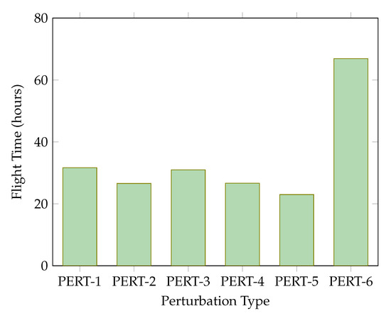
Figure 6.
Best flight time reported for each perturbation in 15 executions.
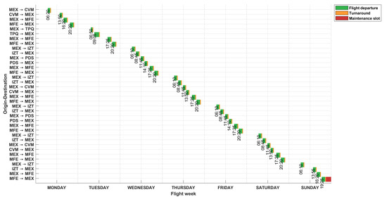
Figure 7.
Representation of the rotation for the best flight time of study case 2.
3.2.2. Maximization of the Number of Flights for Study Case 2
Similarly, Table 12 and Figure 8 present the results of 15 executions for the objective function of maximizing the number of flights. As with the previous objective function, PERT-6 demonstrates the best overall performance. However, in this case, the minimum (worst) number of flights is notably low: only 2 for most perturbations. This suggests that the objective function may not effectively guide the search process. In other words, solutions with identical flight counts are treated equally, even if some have greater potential for improvement. As a result, the algorithm struggles to distinguish between promising and suboptimal solutions.
Table 12.
Study case 2: Aeromar data. Maximization of the number of flights. Results for each perturbation for 15 executions.
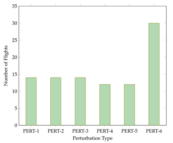
Figure 8.
Study case 2: Aeromar data. The highest number of flights assigned in 15 executions of the algorithm for each of the perturbations.
3.3. Study Case 3: Maintenance Requirement with Mexican Airline Data
In this test, the data from Test 2 are used with the same parameters, but a minimum of two maintenance events is enforced throughout each rotation by setting to 2. This configuration aims not only to satisfy the objective functions and constraints but also to promote a greater frequency of maintenance opportunities due to the forced requirement.
3.3.1. Flight Time Maximization with Two Maintenance Events for Study Case 3
Table 13 presents the results for the flight time objective function. Across all perturbations, flight times generally decrease compared to the previous test, likely due to the inclusion of two mandatory maintenance stops, which limit the search space and reduce total flight duration. Nevertheless, PERT-6 achieves a flight time of 60 h 5 min across five destinations, exceeding the average range of the fleet, indicating a positive outcome for flight time maximization. This rotation, presented in Figure 9, also includes four maintenance opportunities. Conversely, schedule perturbation (PERT-2) yields less favorable results, as rotations exhibit reduced flight durations, as shown in Figure 10.
Table 13.
Total flight time for study case 3, all the rotations present, at least 2 maintenance windows.
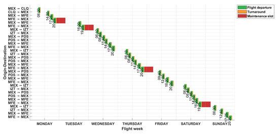
Figure 9.
Representation of the rotation for the best flight time for study case 3.
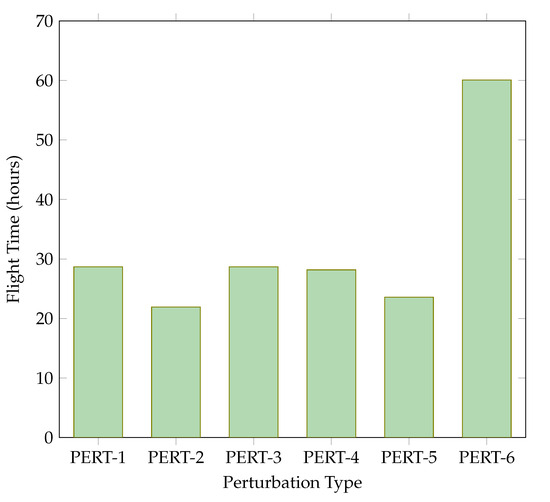
Figure 10.
Best total flight time for study case 3 for each perturbation.
3.3.2. Maximization of the Number of Flights with Two Maintenance Events for Study Case 3
According to the results of the objective function of the number of flights shown in Table 14, most perturbations do not yield more than 14 flights. However, as illustrated in Figure 11, PERT-6 achieves a total of 28 flights during the week. Although this value is lower than that obtained in the previous test, it remains within the typical weekly flight range for the airline’s fleet. The maintenance opportunities recorded in this test, presented in Table 15 and Table 16, indicate that all solutions present at least two maintenance events for both objective functions, except for PERT-3, where there is no feasible solution in an execution. Among the two, the flight-time objective function consistently generates a greater number of maintenance opportunities than the objective function of the number of flights. Table 17 summarizes computation time executions for the experiments of study cases 2 and 3. We can observe that the algorithm employing the implementation of the objective function, which involves the number of flights, achieves a lower average execution time.
Table 14.
Results of the objective function of the number of flights for study case 3.
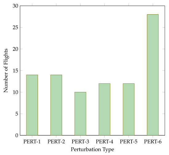
Figure 11.
Best total flight time for study case 3.
Table 15.
Maintenance opportunities for 15 executions of the algorithm maximizing time flight for study case 3.
Table 16.
Results maintenance opportunities for number of flights, study case 3.
Table 17.
Mean of the computation time executions for study cases 2 and 3.
3.4. Summary of Perturbation Performance
Table 18 shows the result of applying the Wilcoxon test. The alternative hypothesis is that the objective function values reported by perturbation 6 are greater than those reported by the other perturbations. In all the cases, the null hypothesis is rejected with small p-values. Notice that the greater p-value is less than 0.1%; hence, the conclusion is statistically significant.
Table 18.
p-values from Wilcoxon hypothesis test. The alternative hypothesis is that the objective function values reported by perturbation 6 are greater than those reported by the other perturbations. Null hypothesis is clearly rejected for all cases.
4. Conclusions
This article presents optimization models for airline route design, along with a set of perturbation operators designed to enhance candidate solutions through simulated annealing. As noted above, most direct search algorithms, such as metaheuristics such as particle swarm optimization, genetic algorithms, differential evolution, and estimation of distribution algorithms, rely heavily on perturbation operators. Consequently, the proposed operators can be readily integrated into a wide range of optimization frameworks.
The results indicate that the best performance is achieved when combining multiple types of perturbations. Specifically, the most effective operator, PERT-6, applies one of the other perturbations at random with the following probabilities: PERT-3 at 0.09, PERT-1 at 0.18, PERT-2 at 0.18, PERT-5 at 0.45, and a final perturbation at 0.10. These operators do not always make drastic or uniform changes. For example, PERT-5, which is applied with the highest probability, modifies the departure schedule by shifting a flight to the next or previous available time slot. In addition, the flight-time maximization objective consistently produces feasible solutions and exhibits a larger variance between the best and worst outcomes across operators; hence, it is inferred that it produces the largest improvements from the initial solution to the final solution. This behavior suggests that the objective function provides strong guidance during the search process, as most changes in a rotation translate directly into measurable differences in flight time. In contrast, the number of flights objective function often yields fewer changes, even when substantial modifications are made to the rotation, thereby limiting the algorithm’s ability to distinguish between solutions. These observations suggest two key directions: perturbation operators should integrate a diverse range of modification types, including substitution, elimination, and addition of flights and schedules, and they should vary the intensity of these modifications, such as the number of flights altered and the extent of schedule shifts.
The proposed method demonstrates its ability to generate competitive solutions, even when applied to real-world scenarios. However, certain requirements, such as prioritizing flight connections and enforcing coverage of all possible destinations, are not currently included in the objective function. However, we outline how these can be incorporated using penalization strategies, similar to the penalty applied for violating the rotation period constraint.
Hard constraints, such as path and closed path requirements, are addressed by enforcing the generation of feasible candidate solutions or through repair procedures. We distinguish two scenarios for constraint handling: (1) when a constraint violation may lead to an improved solution, as in the case where the rotation duration exceeds the rotation period, a penalization approach is appropriate; and (2) when a constraint violation does not yield useful solutions, such as disconnected flight sequences in the case of path or closed-path violations, the constraint must be strictly enforced during solution construction or through repair mechanisms.
In contrast to standard approaches such as linearized or hybrid approaches, the current proposal handles a variable-sized rotation, discrete departure times, and maintenance time slots without forcing a particular time or airport. Instead, given a set of airports, the optimizer selects the times allowing for an arbitrarily long rotation period without constraining the number of repeated flights. Most approaches constraint the rotation period to a day or three days and avoid repeating flights or airports to facilitate optimization by a linear optimizer. Hence, this proposal is suitable for tackling a realistic problem and scaling to additional constraints or objectives without requiring essential modifications, such as maximizing profits.
Overall, the method produces rotation plans that resemble those used by the airline while also satisfying additional requirements such as the allocation of maintenance time slots. The approach shows promise in accommodating more complex constraints and scaling to larger datasets involving more airports, connections, and schedules. Future work will focus on developing optimization models that incorporate additional requirements, such as prioritizing or weighting flight connections, and alternative objectives, including revenue maximization. In addition, we plan to evaluate multiple optimization algorithms to identify those that consistently perform well in this context.
Author Contributions
Conceptualization, S.I.V. and E.E.H.; methodology, S.I.V.; implementation, A.I.D.-M.; validation, A.I.D.-M. and S.I.V.; formal analysis, A.I.D.-M. and S.I.V.; investigation, E.E.H.; resources, E.E.H.; data curation, A.I.D.-M.; writing—original draft preparation, A.I.D.-M. and S.I.V.; writing—review and editing, S.I.V. and E.E.H.; visualization, S.I.V.; supervision, E.E.H.; project administration, S.I.V. and E.E.H.; funding acquisition, E.E.H. All authors have read and agreed to the published version of the manuscript.
Funding
This work was partially supported by the project SIP20250771.
Institutional Review Board Statement
Not applicable.
Informed Consent Statement
Not applicable.
Data Availability Statement
The dataset used in this study is publicly available [github] at https://github.com/EEHMatNMSU/Flight-Routing-Optimization-with-Maintenance-Constraints.git (accessed on 10 August 2025).
Acknowledgments
Eusebio E. Hernandez thanks the IPN for the support during their sabbatical leave.
Conflicts of Interest
The authors declare no conflicts of interest.
References
- Kinnison, H.A.; Siddiqui, T. Aviation Maintenance Management; McGraw-Hill Education: Columbus, OH, USA, 2013. [Google Scholar]
- Barnhart, C.; Boland, N.L.; Clarke, L.W.; Johnson, E.L.; Nemhauser, G.L.; Shenoi, R.G. Flight string models for aircraft fleeting and routing. Transp. Sci. 1998, 32, 208–220. [Google Scholar] [CrossRef]
- Sriram, C.; Haghani, A. An optimization model for aircraft maintenance scheduling and re-assignment. Transp. Res. Part A Policy Pract. 2003, 37, 29–48. [Google Scholar] [CrossRef]
- Sarac, A.; Batta, R.; Rump, C.M. A branch-and-price approach for operational aircraft maintenance routing. Eur. J. Oper. Res. 2006, 175, 1850–1869. [Google Scholar] [CrossRef]
- Liang, Z.; Chaovalitwongse, W.; Huang, H.; Johnson, E. On a New Rotation Tour Network Model for Aircraft Maintenance Routing Problem. Transp. Sci. 2011, 45, 109–120. [Google Scholar] [CrossRef]
- Haouari, M.; Shao, S.; Sherali, H.D. A Lifted Compact Formulation for the Daily Aircraft Maintenance Routing Problem. Transp. Sci. 2013, 47, 508–525. [Google Scholar] [CrossRef]
- Başdere, M.; Bilge, Ü. Operational aircraft maintenance routing problem with remaining time consideration. Eur. J. Oper. Res. 2014, 235, 315–328. [Google Scholar] [CrossRef]
- Al-Thani, N.A.; Ahmed, M.B.; Haouari, M. A model and optimization-based heuristic for the operational aircraft maintenance routing problem. Transp. Res. Part C—Emerg. Technol. 2016, 72, 29–44. [Google Scholar] [CrossRef]
- Eltoukhy, A.; Chan, F.; Chung, S.H.; Niu, B.; Wang, X. Heuristic approaches for operational aircraft maintenance routing problem with maximum flying hours and man-power availability considerations. Ind. Manag. Data Syst. 2017, 117, 2142–2170. [Google Scholar] [CrossRef]
- Safaei, N.; Jardine, A.K. Aircraft routing with generalized maintenance constraints. Omega 2018, 80, 111–122. [Google Scholar] [CrossRef]
- Eltoukhy, A.E.; Chan, F.T.; Chung, S.; Niu, B. A model with a solution algorithm for the operational aircraft maintenance routing problem. Comput. Ind. Eng. 2018, 120, 346–359. [Google Scholar] [CrossRef]
- Sanchez, D.T.; Boyacı, B.; Zografos, K.G. An optimisation framework for airline fleet maintenance scheduling with tail assignment considerations. Transp. Res. Part B Methodol. 2020, 133, 142–164. [Google Scholar] [CrossRef]
- Ruan, J.; Wang, Z.; Chan, F.T.; Patnaik, S.; Tiwari, M. A reinforcement learning-based algorithm for the aircraft maintenance routing problem. Expert Syst. Appl. 2021, 169, 114399. [Google Scholar] [CrossRef]
- Bulbul, K.G.; Kasimbeyli, R. Augmented Lagrangian based hybrid subgradient method for solving aircraft maintenance routing problem. Comput. Oper. Res. 2021, 132, 105294. [Google Scholar] [CrossRef]
- Zhang, Q.; Chan, F.T.; Chung, S.H.; Fu, X. A matheuristic for aircraft maintenance routing problem incorporating cruise speed control. Expert Syst. Appl. 2024, 242, 122711. [Google Scholar] [CrossRef]
- Saltzman, R.M.; Stern, H.I. The multi-day aircraft maintenance routing problem. J. Air Transp. Manag. 2022, 102, 102224. [Google Scholar] [CrossRef]
- Alpos, T.; Iliopoulou, C.; Kepaptsoglou, K. Nature-Inspired Optimal Route Network Design for Shared Autonomous Vehicles. Vehicles 2023, 5, 24–40. [Google Scholar] [CrossRef]
- Zacharia, P.; Stavrinidis, S. The Vehicle Routing Problem with Simultaneous Pick-Up and Delivery under Fuzziness Considering Fuel Consumption. Vehicles 2024, 6, 231–241. [Google Scholar] [CrossRef]
- Kouretas, K.; Kepaptsoglou, K. Planning Integrated Unmanned Aerial Vehicle and Conventional Vehicle Delivery Operations under Restricted Airspace: A Mixed Nested Genetic Algorithm and Geographic Information System-Assisted Optimization Approach. Vehicles 2023, 5, 1060–1086. [Google Scholar] [CrossRef]
- Peng, Y.; Zhu, W.; Yu, D.Z.; Liu, S.; Zhang, Y. Multi-Depot Electric Vehicle–Drone Collaborative-Delivery Routing Optimization with Time-Varying Vehicle Travel Time. Vehicles 2024, 6, 1812–1842. [Google Scholar] [CrossRef]
- Moradi, N.; Wang, C.; Mafakheri, F. Urban Air Mobility for Last-Mile Transportation: A Review. Vehicles 2024, 6, 1383–1414. [Google Scholar] [CrossRef]
- Voigt, S. A review and ranking of operators in adaptive large neighborhood search for vehicle routing problems. Eur. J. Oper. Res. 2025, 322, 357–375. [Google Scholar] [CrossRef]
- Benjelloun, R.; Tarik, M.; Jebari, K. Open Competency Optimization with Combinatorial Operators for the Dynamic Green Traveling Salesman Problem. Information 2025, 16, 675. [Google Scholar] [CrossRef]
- Peng, B.; Zhang, Y.; Gajpal, Y.; Chen, X. A Memetic Algorithm for the Green Vehicle Routing Problem. Sustainability 2019, 11, 6055. [Google Scholar] [CrossRef]
- Rezvanian, S.; Husseinzadeh Kashan, A.; Rezvanian, A.; Sabzevari, A. Intelligent vehicle routing for stochastic service times: A grouping evolution strategy approach. Int. J. Transp. Sci. Technol. 2025. in press. [CrossRef]
- Liu, X.; Chen, Y.L.; Por, L.Y.; Ku, C.S. A Systematic Literature Review of Vehicle Routing Problems with Time Windows. Sustainability 2023, 15, 12004. [Google Scholar] [CrossRef]
- Gopalan, R.; Talluri, K.T. The aircraft maintenance routing problem. Oper. Res. 1998, 46, 260–271. [Google Scholar] [CrossRef]
- Peres, F.; Castelli, M. Combinatorial optimization problems and metaheuristics: Review, challenges, design, and development. Appl. Sci. 2021, 11, 6449. [Google Scholar] [CrossRef]
- Sánchez, M.; Cruz-Duarte, J.M.; carlos Ortíz-Bayliss, J.; Ceballos, H.; Terashima-Marin, H.; Amaya, I. A systematic review of hyper-heuristics on combinatorial optimization problems. IEEE Access 2020, 8, 128068–128095. [Google Scholar] [CrossRef]
- Cruz-Rosales, M.H.; Cruz-Chávez, M.A.; Alonso-Pecina, F.; Peralta-Abarca, J.d.C.; Ávila-Melgar, E.Y.; Martínez-Bahena, B.; Enríquez-Urbano, J. Metaheuristic with cooperative processes for the university course timetabling problem. Appl. Sci. 2022, 12, 542. [Google Scholar] [CrossRef]
- Kirkpatrick, S.; Gelatt, C.D., Jr.; Vecchi, M.P. Optimization by simulated annealing. Science 1983, 220, 671–680. [Google Scholar] [CrossRef]
- Díaz-Molina, A.I.; Valdez, S.I.; Hernández, E.E. Code for the Article: Flight Routing Optimization with Maintenance Constraints. 2025. Available online: https://github.com/EEHMatNMSU/Flight-Routing-Optimization-with-Maintenance-Constraints.git (accessed on 10 August 2025).
- Bazargan, M. Airline Operations and Scheduling, 2nd ed.; Ashgate Publishing Company: London, UK, 2010. [Google Scholar]
- Airportinfo.live. Aeromar Estado de Vuelos, n.d. Available online: https://airportinfo.live/es/estado-de-vuelos-aeromar (accessed on 10 January 2023).


Disclaimer/Publisher’s Note: The statements, opinions and data contained in all publications are solely those of the individual author(s) and contributor(s) and not of MDPI and/or the editor(s). MDPI and/or the editor(s) disclaim responsibility for any injury to people or property resulting from any ideas, methods, instructions or products referred to in the content. |
© 2025 by the authors. Licensee MDPI, Basel, Switzerland. This article is an open access article distributed under the terms and conditions of the Creative Commons Attribution (CC BY) license (https://creativecommons.org/licenses/by/4.0/).