
Evaluation of the Energy Equivalent Speed of Car Damage Using a Finite Element Model


Abstract
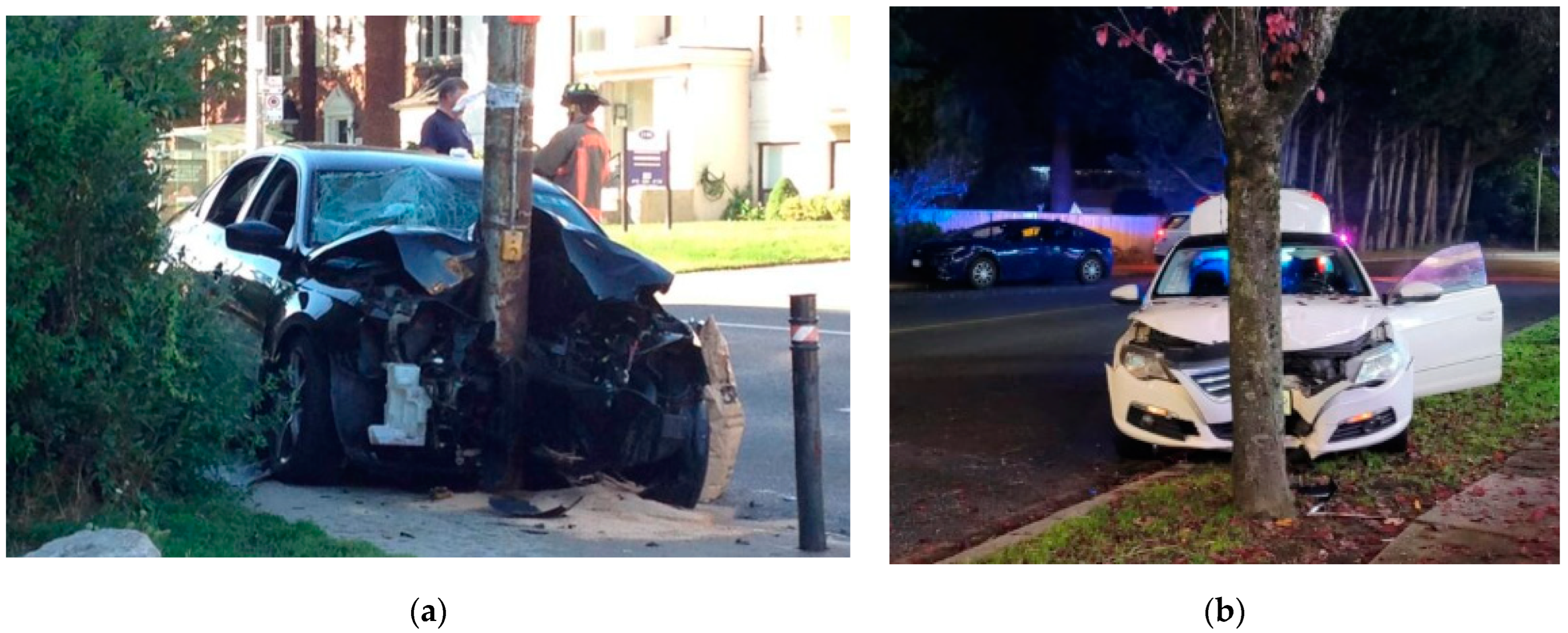
1. Introduction
2. Overview of the Methods for Estimating the EES of Vehicle Damage
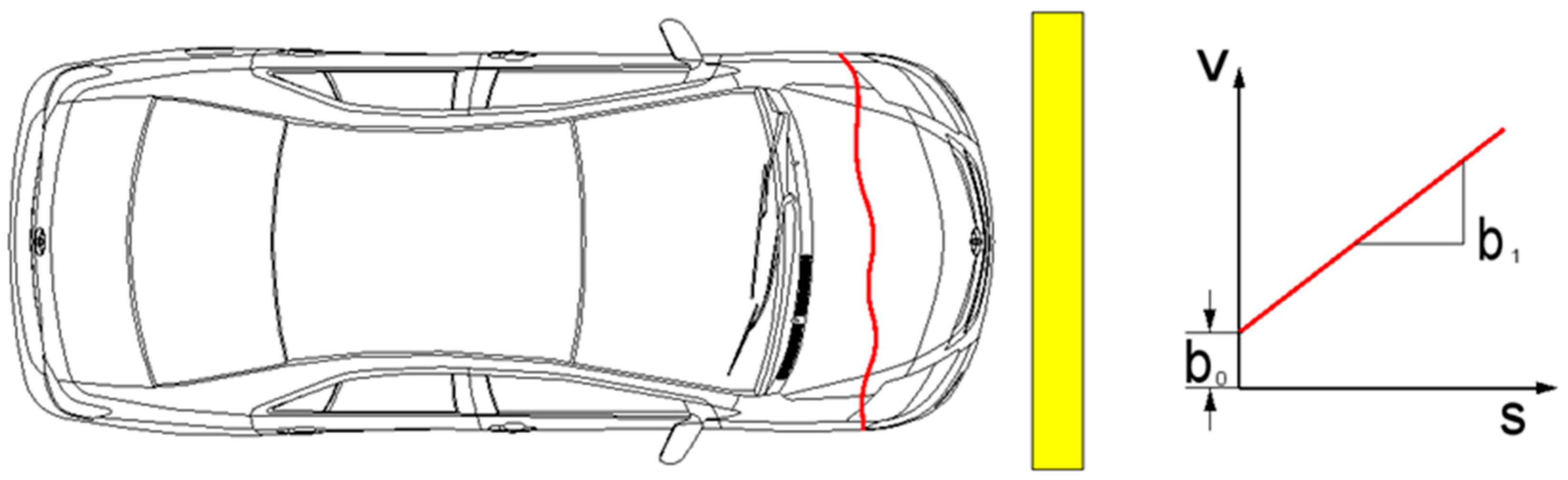
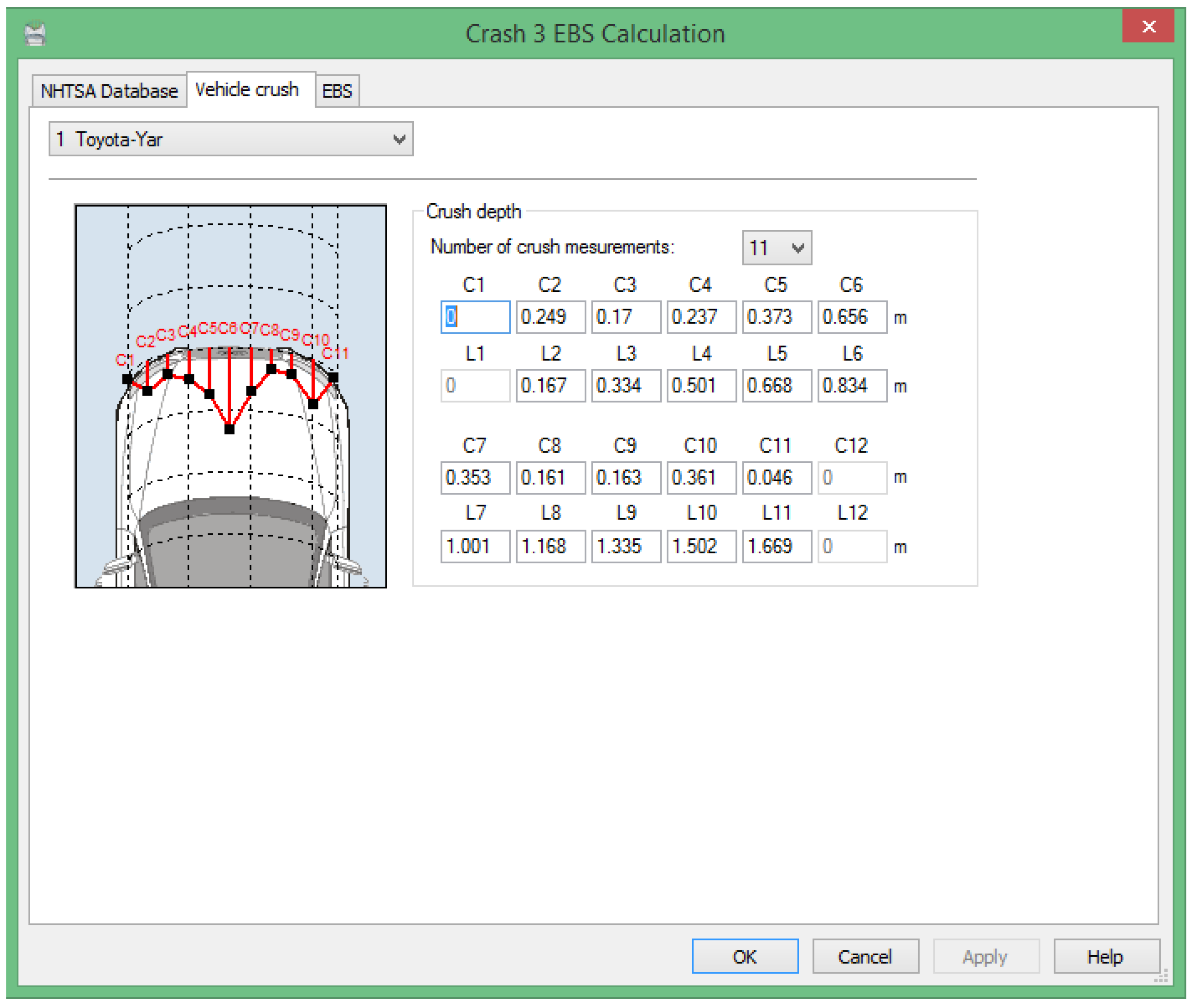
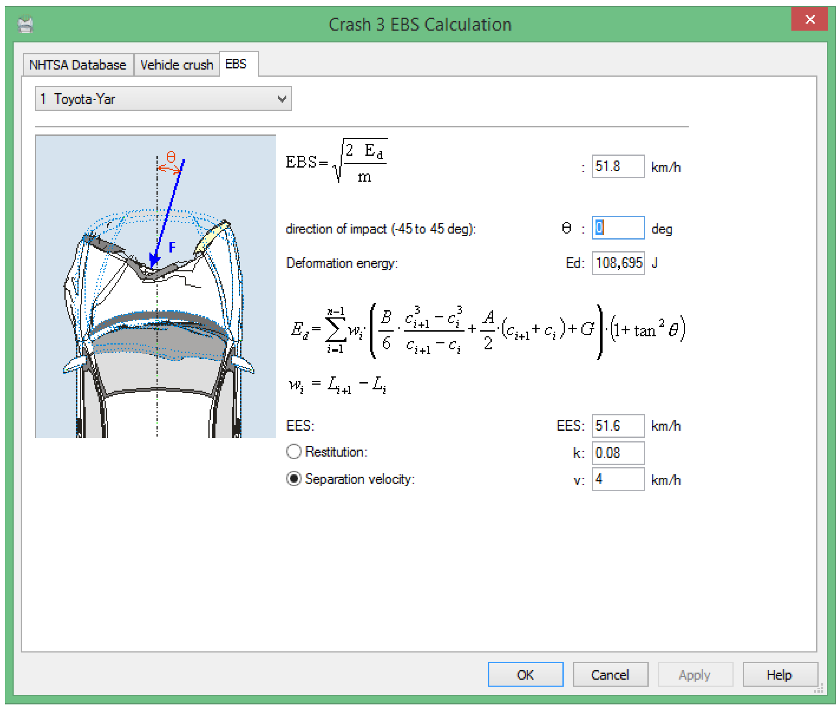
2.1. Methodology for Calculating the Deformation Energy Based on Deformation Size
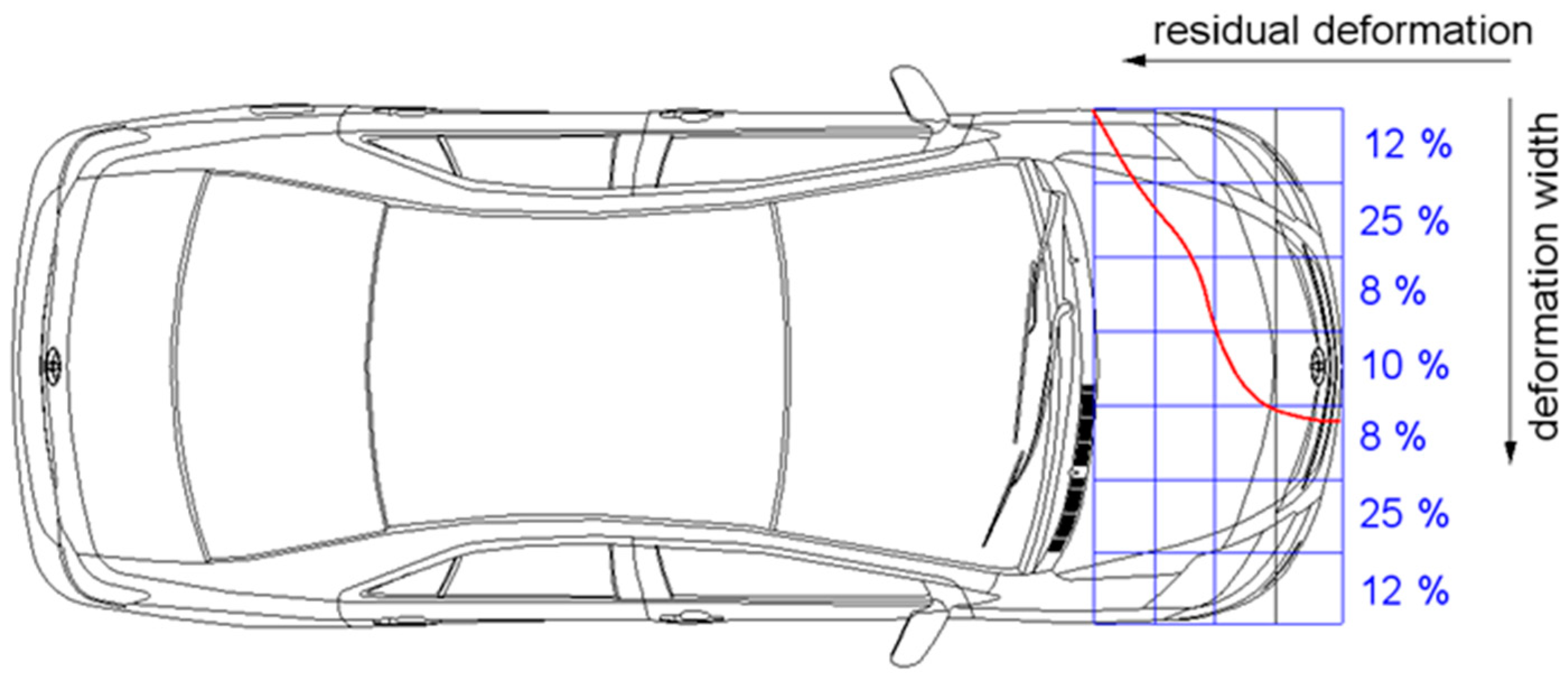
2.2. Calculation of the EES Parameter Based on the Deformed Volume
- (1)
- 9.0 × 10⁵…11 × 105 N/mm2, when the car strength structure was broken as a result of the deformations;
- (2)
- 2.0 × 10⁵…4.0 × 10⁵ N/mm2, when the deformations are located only in the skin plate elements;
- (3)
- When the car strength structure was broken:
- (a)
- 13.5 × 10⁵…22.6 × 10⁵ N/mm2 for small cars;
- (b)
- 9.1 × 10⁵…13.5 × 10⁵ N/mm2 for medium cars;
- (c)
- 5.2 × 10⁵…7.2 × 10⁵ N/mm2 for large cars.
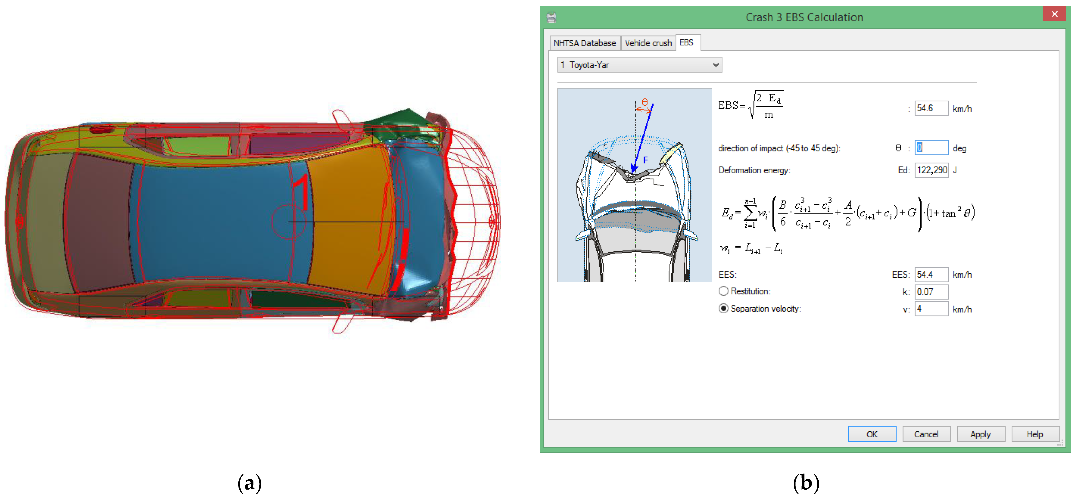
2.3. Application of the EES Catalog to Estimating the Energy Equivalent
2.4. Analysis of the Methods Used to Estimate the Energy Equivalent of Vehicle Damage When Hitting a Utility Pole or a Tree
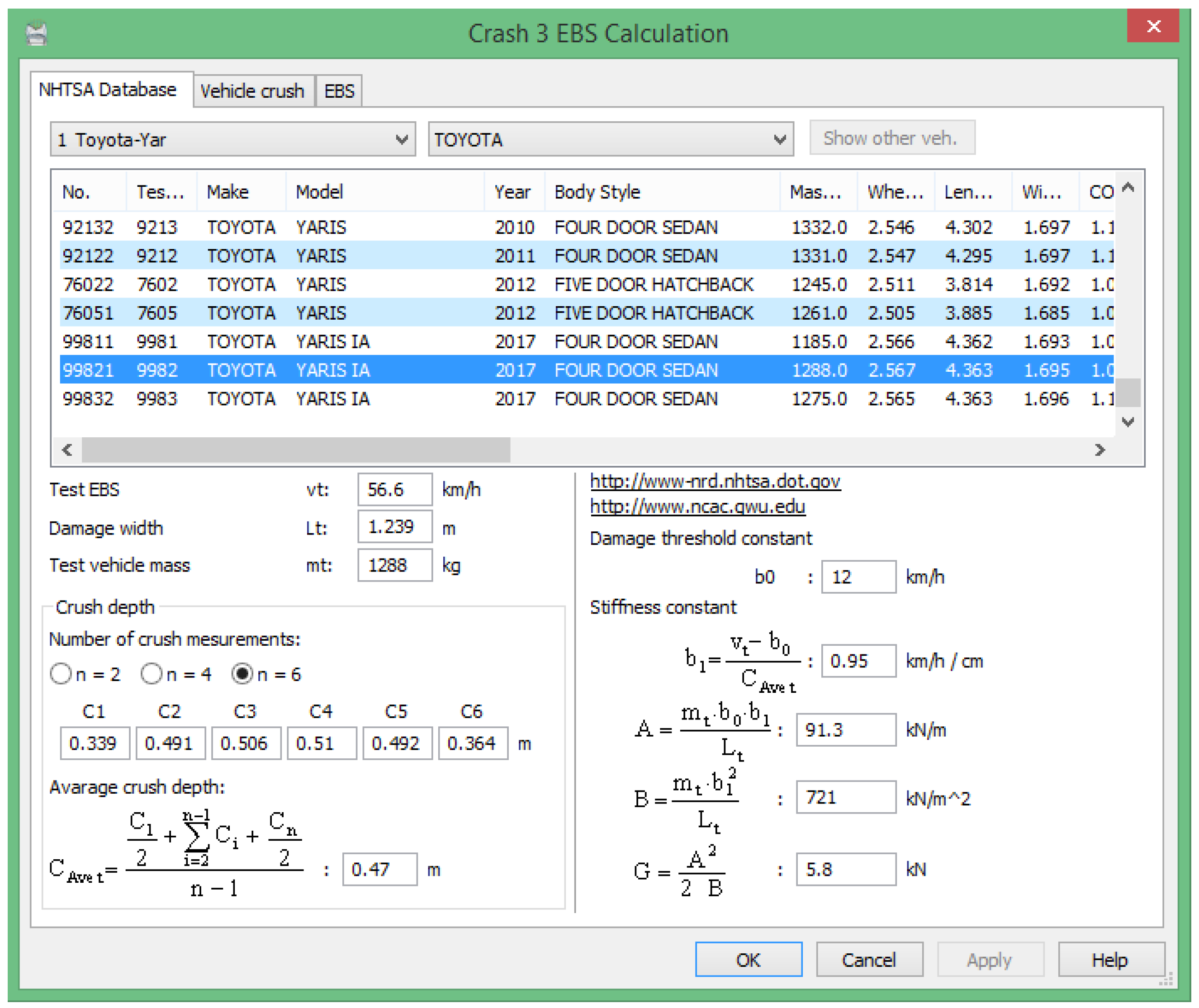
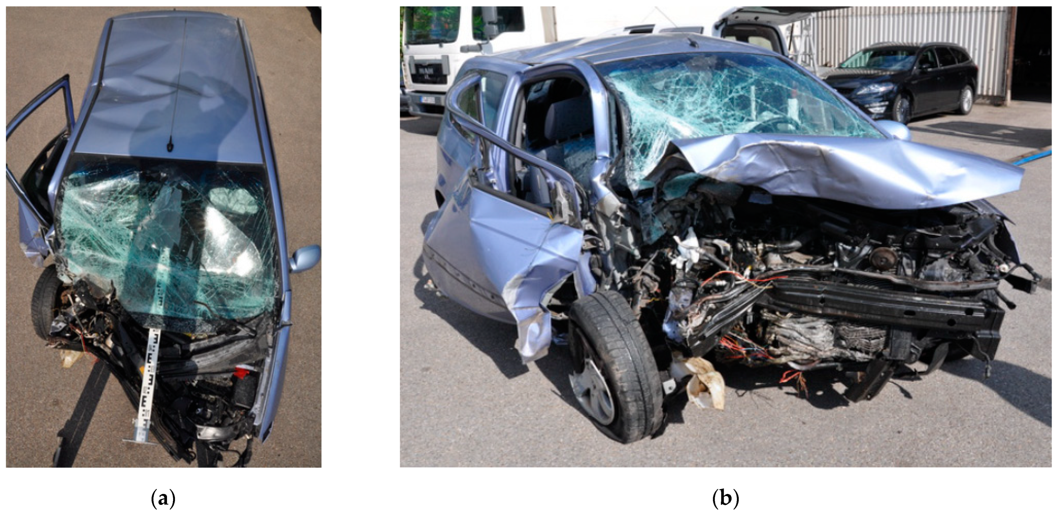
3. Evaluation of the Energy Equivalent of Vehicle Damage Using LS DYNNA
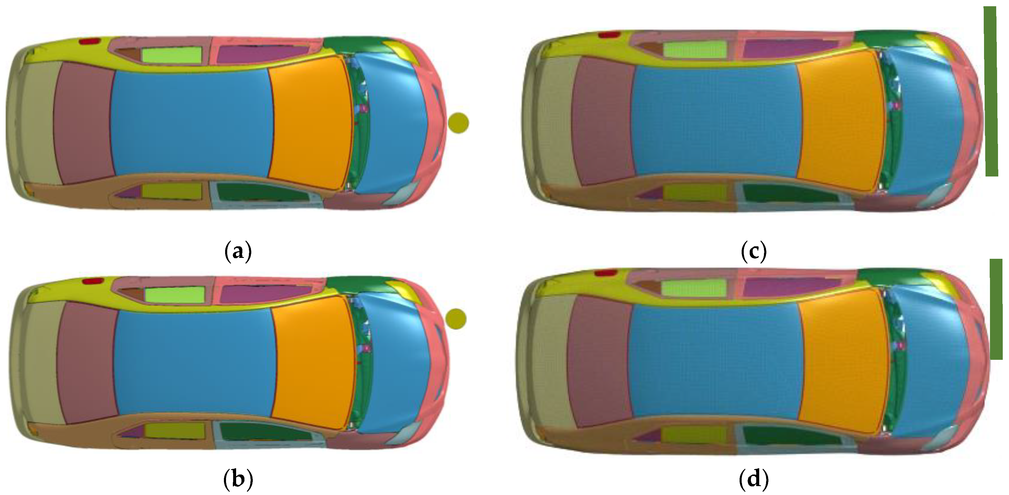
Simulation of a Collision with a Fixed Object and a Non-Deformable Wall
4. Results
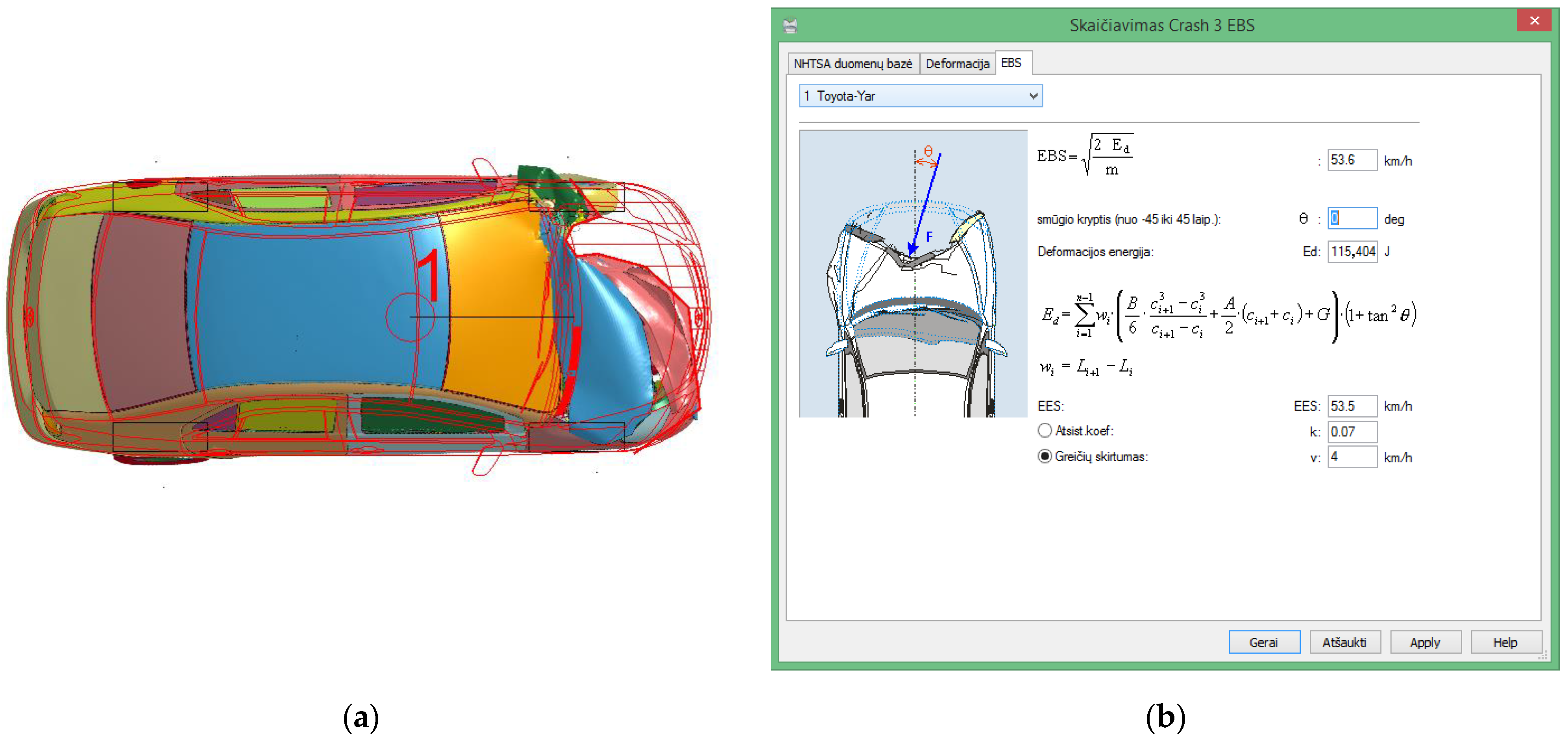
4.1. Deformation Analysis
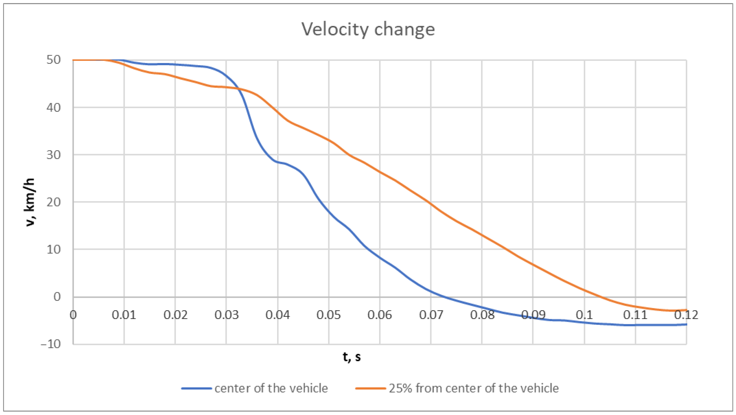
4.2. Speed Variation Analysis
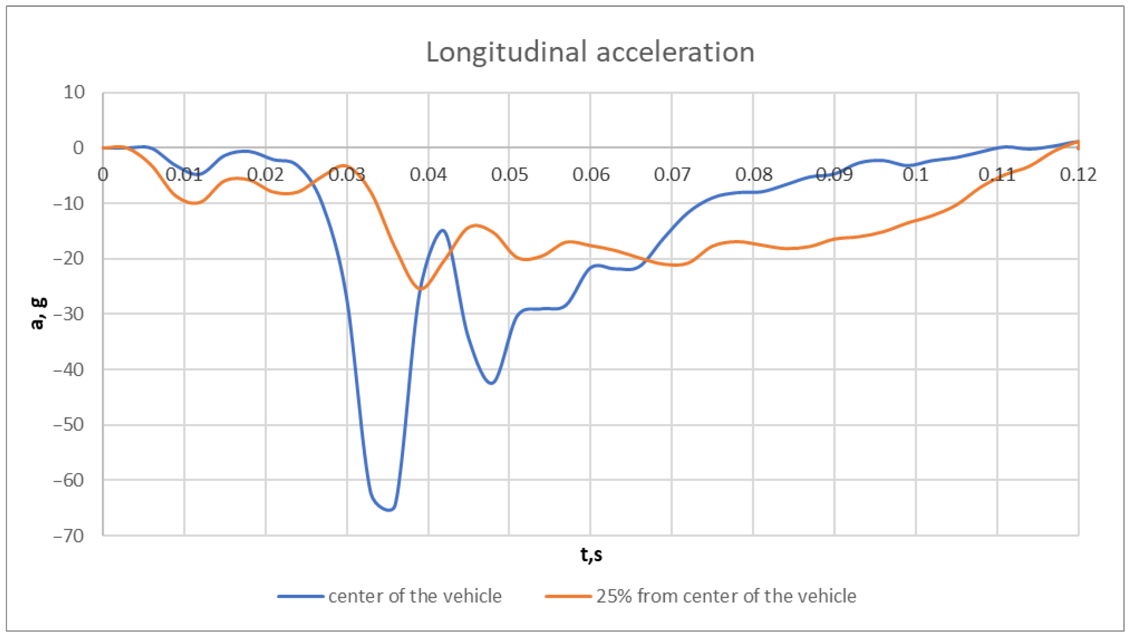
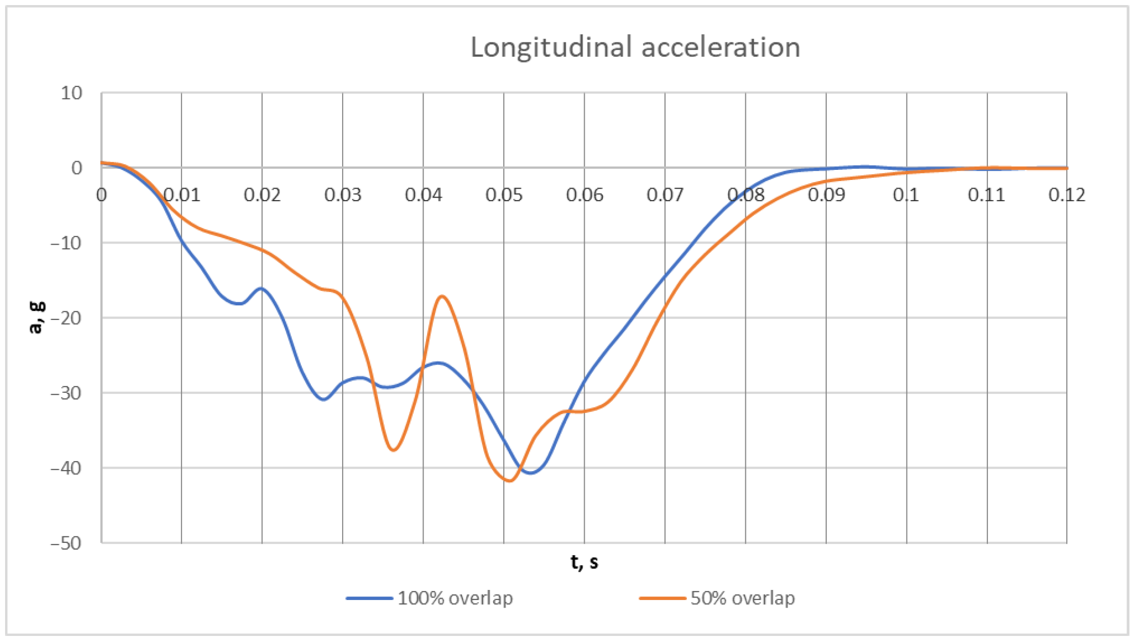
4.3. Longitudinal Acceleration Analysis
4.4. Speed Adjustment
5. Conclusions
Author Contributions
Funding
Data Availability Statement
Conflicts of Interest
References
- World Health Organization. Global Status Report on Road Safety 2023; World Health Organization: Geneva, Switzerland, 2023; ISBN 978-92-4-008651-7.
- Chang, F.-R.; Huang, H.-L.; Schwebel, D.C.; Chan, A.H.S.; Hu, G.-Q. Global Road Traffic Injury Statistics: Challenges, Mechanisms and Solutions. Chin. J. Traumatol. 2020, 23, 216–218. [Google Scholar] [CrossRef]
- Gidlewski, M.; Prochowski, L.; Jemioł, L.; Żardecki, D. The Process of Front-to-Side Collision of Motor Vehicles in Terms of Energy Balance. Nonlinear Dyn. 2019, 97, 1877–1893. [Google Scholar] [CrossRef]
- Burg, H.; Moser, A. (Eds.) Handbuch Verkehrsunfallrekonstruktion: Unfallaufnahme, Fahrdynamik, Simulation; ATZ/MTZ-Fachbuch; 3. aktualisierte Auflage; Springer Vieweg: Wiesbaden, Germany, 2017; ISBN 978-3-658-16142-2. [Google Scholar]
- Vangi, D. Energy Loss in Vehicle to Vehicle Oblique Impact. Int. J. Impact Eng. 2009, 36, 512–521. [Google Scholar] [CrossRef]
- Kubiak, P.; Siczek, K.; Dąbrowski, A.; Szosland, A. New High Precision Method for Determining Vehicle Crash Velocity Based on Measurements of Body Deformation. Int. J. Crashworthiness 2016, 21, 532–541. [Google Scholar] [CrossRef]
- Breitlauch, P.; Erbsmehl, C.T.; Van Ratingen, M.; Mallada, J.L.; Sandner, V.; Ferson, N.; Urban, M. A Novel Method for the Automated Simulation of Various Vehicle Collisions to Estimate Crash Severity. Traffic Inj. Prev. 2023, 24, S116–S123. [Google Scholar] [CrossRef] [PubMed]
- Vangi, D.; Begani, F. Energy Loss in Vehicle Collisions from Permanent Deformation: An Extension of the ‘Triangle Method’. Veh. Syst. Dyn. 2013, 51, 857–876. [Google Scholar] [CrossRef]
- Mackay, G.M.; Hill, J.; Parkin, S.; Munns, J.A.R. Restrained Occupants on the Nonstruck Side in Lateral Collisions. Accid. Anal. Prev. 1993, 25, 147–152. [Google Scholar] [CrossRef] [PubMed]
- Uddin, M.S.; Quintel, J.; Zivkovic, G. On the Design of Energy Absorbing Crash Buffers for High Speed Roadways. Open J. Saf. Sci. Technol. 2016, 06, 11–24. [Google Scholar] [CrossRef]
- Alardhi, M.; Sequeira, R.; Melad, F.; Alrajhi, J.; Alkhulaifi, K. Crashworthiness Analysis to Evaluate the Performance of TDM-Shielded Street Poles Using FEA. Appl. Sci. 2023, 13, 4393. [Google Scholar] [CrossRef]
- Zheng, L.; Sayed, T. Utility Poles. In International Encyclopedia of Transportation; Elsevier: Amsterdam, The Netherlands, 2021; pp. 731–736. ISBN 978-0-08-102672-4. [Google Scholar]
- IIHS. Collisions with Fixed Objects and Animals 2023. Available online: https://www.iihs.org/topics/fatality-statistics/detail/collisions-with-fixed-objects-and-animals#fn1 (accessed on 10 January 2024).
- Baranowski, P.; Damaziak, K. Numerical Simulation of Vehicle–Lighting Pole Crash Tests: Parametric Study of Factors Influencing Predicted Occupant Safety Levels. Materials 2021, 14, 2822. [Google Scholar] [CrossRef]
- Ispas, N.; Nastasoiu, M. Analysis of Car’s Frontal Collision against Pole. IOP Conf. Ser. Mater. Sci. Eng. 2017, 252, 012012. [Google Scholar] [CrossRef]
- Campbell, K.L. Energy Basis for Collision Severity. SAE Trans. 1974, 83, 2114–2126. [Google Scholar]
- Kubiak, P.; Mierzejewska, P.; Szosland, A. A Precise Method of Vehicle Velocity Determination Based on Measurements of Car Body Deformation—Non-Linear Method for the ‘Luxury’ Vehicle Class. Int. J. Crashworthiness 2018, 23, 100–107. [Google Scholar] [CrossRef]
- Dr. Steffan PC Crash. DSD ReconData 2018. Available online: https://www.dsd.at/index.php?option=com_content&view=article&id=512:pc-crash-englisch-3&catid=37&lang=en&Itemid=159 (accessed on 20 February 2024).
- Wach, W. Symulacja Wypadków Drogowych w Programie PC-Crash; Wydawnictwo Instytutu Ekspertyz Sądowych: Kraków, Poland, 2009; ISBN 978-83-87425-23-4. [Google Scholar]
- Niehoff, P. The Accuracy of Energy-Based Crash Reconstruction Techniques Using e Using Event Data r Ent Data Recorder Measur Der Measurements. Master’s Thesis, Rowan University, Glassboro, NJ, USA, 2005. [Google Scholar]
- Prochowski, L.; Unarski, J.; Wach, W.; Wicher, J. (Eds.) Podstawy Rekonstrukcji Wypadków Drogowych; Pojazdy Samochodowe; Wyd. 2. uaktualnione; Wydawnictwa Komunikacji i Łączności: Warszawa, Poland, 2014; ISBN 978-83-206-1940-9. [Google Scholar]
- Kubiak, P.; Wozniak, M.; Ozuna, G. Determination of the Energy Necessary for Cars Bodydeformation by Application of the NHTSA Stifness Coefficient. Mach. Technol. Mater. 2014, VIII, 38–40. [Google Scholar]
- Moravcová, P.; Bucsuházy, K.; Bilík, M.; Belák, M.; Bradáč, A. Let It Crash! Energy Equivalent Speed Determination. In Proceedings of the 7th International Conference on Vehicle Technology and Intelligent Transport Systems, Virtual, 28–30 April 2021; SCITEPRESS—Science and Technology Publications. pp. 521–528. [Google Scholar]
- Bucsuházy, K.; Matuchová, E.; Zůvala, R.; Moravcová, P.; Kostíková, M.; Mikulec, R. Human Factors Contributing to the Road Traffic Accident Occurrence. Transp. Res. Procedia 2020, 45, 555–561. [Google Scholar] [CrossRef]
- Macurová, Ľ.; Kohút, P.; Čopiak, M.; Imrich, L.; Rédl, M. Determinig the Energy Equivalent Speed by Using Software Based on the Finite Element Method. Transp. Res. Procedia 2020, 44, 219–225. [Google Scholar] [CrossRef]
- Cofone, J.N.; Rich, A.S.; Scott, C.A. A Comparison of Equations for Estimating Speed Based on Maximum Static Deformation for Frontal Narrow-Object Impacts. Accid. Reconstr. J. 2007, 11, 19–27. [Google Scholar]
- Nystrom, G.A.; Kost, G. Application of the NHTSA Crash Database to Pole Impact Predictions. SAE Tech. Pap. 1992, 920605. [Google Scholar]
- Craig, V. Analysis of Pole Barrier Test Data and Impact Equations. Accid. Reconstr. J. 1993, 9. [Google Scholar]
- Burdzik, R.; Folęga, P.; Konieczny, Ł.; Łazarz, B.; Stanik, Z.; Warczek, J. Analysis of Material Deformation Work Measures in Determination of a Vehicle’s Collision Speed. Arch. Matrials Sci. Eng. 2012, 58, 13–21. [Google Scholar]
- Noorsumar, G.; Rogovchenko, S.; Robbersmyr, K.G.; Vysochinskiy, D. Mathematical Models for Assessment of Vehicle Crashworthiness: A Review. Int. J. Crashworthiness 2022, 27, 1545–1559. [Google Scholar] [CrossRef]
- Goehner, U. Car Crash Simulations and Occupant Safety with LS-DYNA. In Proceedings of the EnginSoft International Conference 2009, Bergamo, Italy, 1–2 October 2009. [Google Scholar]
- Stein, M.; Schwanitz, P.; Sankarasubramanian, H. Unified Parametric Car Model—A Simplified Model for Frontal Crash Safety; DYNAmore GmbH: Ulm, Germany, 2012. [Google Scholar]
- Mertler, S.; Borsotto, D.; Jansen, L.; Thole, C.-A. Combined Analysis of Ls-Dyna Crash-Simulations and Crash-Test Scans. In Proceedings of the 15th International LS-DYNA® Users Conference, Dearborn, MI, USA, 10–12 June 2018. [Google Scholar]
- Reichert, R.; Park, C.; Morgan, R.M. Development of Integrated Vehicle-Occupant Model for Crashworthiness Safety Analysis; National Highway Traffic Safety Administration: Washington, DC, USA, 2014; p. 106.
- Lin, Y.-Y. Performance of LS-DYNA with Double Precision on Linux and Windows CCS. In Proceedings of the 6th European LS-DYNA Users’ Conference, Gothenburg, Sweden, 29–30 May 2007. [Google Scholar]
- Zhang, J.; Wang, L.; Wang, T.; Sun, H.; Zou, X.; Yuan, L. Frontal Crashworthiness Optimization for a Light-Duty Vehicle Based on a Multi-Objective Reliability Method. Int. J. Crashworthiness 2023, 28, 449–461. [Google Scholar] [CrossRef]
- Wågström, L.; Kling, A.; Norin, H.; Fagerlind, H. A Methodology for Improving Structural Robustness in Frontal Car-to-Car Crash Scenarios. Int. J. Crashworthiness 2013, 18, 385–396. [Google Scholar] [CrossRef]
- Kubiak, P.; Krzemieniewski, A.; Lisiecki, K.; Senko, J.; Szosland, A. Precise Method of Vehicle Velocity Determination Basing on Measurements of Car Body Deformation–Non-Linear Method for ‘Full Size’ Vehicle Class. Int. J. Crashworthiness 2018, 23, 302–310. [Google Scholar] [CrossRef]
 —high quality of EES parameter;
  —medium quality of EES parameter.
—high quality of EES parameter; —medium quality of EES parameter.
—medium quality of EES parameter.
—high quality of EES parameter; —medium quality of EES parameter.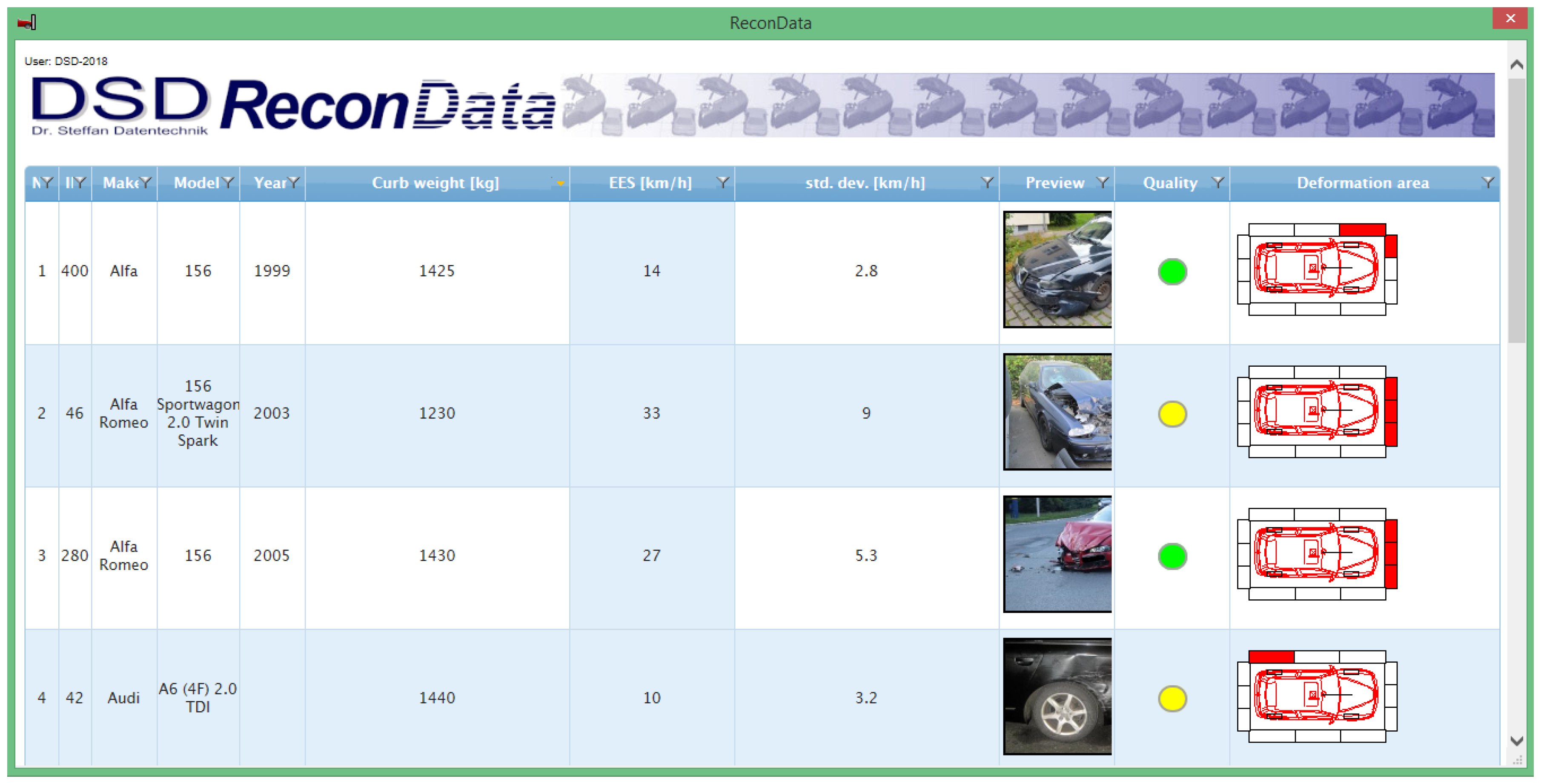


| Vehicle Mass, kg | BP0, km/h | BP1, (km/h)/cm |
|---|---|---|
| 878…1103 | 4.86 | 0.406 |
| 1103…1328 | 3.97 | 0.411 |
| 1328…1553 | 6.50 | 0.380 |
| 1553…1778 | 7.80 | 0.327 |
| 1778…2003 | 6.97 | 0.296 |
| Type of Vehicle | BP0, km/h | BP1 = 0.611 − 0.00005 · mp 1, (km/h)/cm |
|---|---|---|
| With front drive wheels | 8 | 0.57 |
| With rear drive wheels | 8 | 0.51 |
| Type of Vehicle | cmax, cm | EES |
|---|---|---|
| With front drive wheels over 4.6 m in length and over 1360 kg in weight | ≤30.5 | 0.3 · cmax + 6.4 |
| 0.82 · cmax − 9.7 | ||
| For larger cars with front or rear drive wheels | ≥46 | 0.34 · cmax + 6.4 |
| 0.75 · cmax − 11.3 |
| Case of Collision | EES Value Simulated with LS DYNA R.11.0.0, km/h | EES Value According to CRASH 3—EBS Calculation 12.0, km/h | Difference Compared to Simulated Value, % | EES Value According to EES Catalog, km/h | Difference Compared to Simulated Value, % |
|---|---|---|---|---|---|
| Collision with a pole at 25% overlap | 50 | 53.5 | 6.76 | 47.9 | 4.29 |
| Collision with a pole with the impact at the center of the car | 50 | 51.6 | 3.15 | 48.8 | 2.43 |
| Collision with a wall with 100% overlap | 50 | 54.4 | 8.43 | 48.0 | 4.08 |
| Collision with a wall with 50% overlap | 50 | 50.7 | 1.39 | 50.6 | 1.19 |
Disclaimer/Publisher’s Note: The statements, opinions and data contained in all publications are solely those of the individual author(s) and contributor(s) and not of MDPI and/or the editor(s). MDPI and/or the editor(s) disclaim responsibility for any injury to people or property resulting from any ideas, methods, instructions or products referred to in the content. |
© 2024 by the authors. Licensee MDPI, Basel, Switzerland. This article is an open access article distributed under the terms and conditions of the Creative Commons Attribution (CC BY) license (https://creativecommons.org/licenses/by/4.0/).
Share and Cite
Droździel, P.; Pasaulis, T.; Pečeliūnas, R.; Pukalskas, S. Evaluation of the Energy Equivalent Speed of Car Damage Using a Finite Element Model. Vehicles 2024, 6, 632-650. https://doi.org/10.3390/vehicles6020029
Droździel P, Pasaulis T, Pečeliūnas R, Pukalskas S. Evaluation of the Energy Equivalent Speed of Car Damage Using a Finite Element Model. Vehicles. 2024; 6(2):632-650. https://doi.org/10.3390/vehicles6020029
Chicago/Turabian StyleDroździel, Paweł, Tomas Pasaulis, Robertas Pečeliūnas, and Saugirdas Pukalskas. 2024. "Evaluation of the Energy Equivalent Speed of Car Damage Using a Finite Element Model" Vehicles 6, no. 2: 632-650. https://doi.org/10.3390/vehicles6020029
APA StyleDroździel, P., Pasaulis, T., Pečeliūnas, R., & Pukalskas, S. (2024). Evaluation of the Energy Equivalent Speed of Car Damage Using a Finite Element Model. Vehicles, 6(2), 632-650. https://doi.org/10.3390/vehicles6020029