Abstract
Driving style and external factors such as traffic density have a significant influence on the vehicle energy demand especially in city driving. A longitudinal control approach for intelligent, connected vehicles in urban areas is proposed in this article to improve the efficiency of automated driving. The control approach incorporates information from Vehicle-2-Everything communication to anticipate the behavior of leading vehicles and to adapt the longitudinal control of the vehicle accordingly. A supervised learning approach is derived to train a neural prediction model based on a recurrent neural network for the speed trajectories of the ego and leading vehicles. For the development, analysis and evaluation of the proposed control approach, a co-simulation environment is presented that combines a generic vehicle model with a microscopic traffic simulation. This allows for the simulation of vehicles with different powertrains in complex urban traffic environment. The investigation shows that using V2X information improves the prediction of vehicle speeds significantly. The control approach can make use of this prediction to achieve a more anticipatory driving in urban areas which can reduce the energy consumption compared to a conventional Adaptive Cruise Control approach.
1. Introduction
The effects of global climate change are becoming more serious and occurring more frequently in all parts of the world. To mitigate the consequences of climate change in accordance with the Paris climate agreement, the greenhouse gas emissions must be reduced drastically across all sectors. The transportation sector at the moment has a significant share on the total CO2 emission [1]. Despite the concerted efforts towards powertrain concepts that can be powered with renewable energies such as battery electric vehicles or fuel cell electric vehicles, this leads to an immense demand of additional green energies for the operation of a new electric vehicle fleet. According to [2], electric vehicles in European cities have a share of about 11% in 2020, thus the majority of vehicles is still fuel based. Therefore, the simultaneous reduction of energy demand in this area has a significant influence on the efforts against climate change.
Besides the ongoing effort to increase the efficiency of vehicle powertrains, the way vehicles are operated is also a large factor for the overall energy demand. Advanced Driver Assistance Systems can play a significant role in reducing the energy demand in the transportation sector. Especially improving the longitudinal dynamics as the main source of the vehicle’s energy consumption is a major aspect of this effort. According to [3], the energy consumption of electric vehicles is highly dependent on the driving style, for example, driving speed oscillations and a more aggressive acceleration behavior. Longitudinal control systems such as state-of-the-art Adaptive Cruise Control (ACC), are already used by many modern vehicles. The systems used so far have proven their robustness because they are using just in-vehicle information. Improving and extending these systems, especially towards more efficient driving, can be a big step towards the goal to reduce energy consumption for vehicles.
Especially in urban areas with dense traffic and many traffic light systems (TLS), conventional car-following strategies may result in high energy consumption due to frequently occurring stop-and-go situations. In the field of communication technology, Vehicle-2-Everything (V2X) is an emerging concept for inter-vehicle communication (V2V) and communication with the traffic infrastructure (V2I) [4]. V2X communication can provide additional information about relevant traffic parameters which can be incorporated into the control systems in order to predict and ideally avoid such traffic situations. Therefore, information about traffic density or the traffic infrastructure, e.g., traffic lights, can be acquired and used for instance in traffic light advisory systems [5]. Information about the TLS, for example state program and timings, is used in this study in a similar fashion for an intelligent longitudinal control. When processing all of the available data, Machine Learning (ML) has become a key field of research for intelligent vehicle applications. ML models are able to learn complex functional relationships based on large amounts of data in applications in which it is difficult to derive physical models with good performance, such as prediction tasks. Numerous applications for automated and autonomous driving use ML models for a more efficient and safer driving, ranging from perception to different vehicle control aspects such as longitudinal control [6].
The development of such new systems in an urban area along with a representative number of vehicles equipped with the corresponding technology is very expensive. Simulative environments offer an efficient and convenient way to develop intelligent vehicle functionality, but are generally based on many assumptions and simplifications. Especially microscopic traffic simulations such as Simulation of Urban Mobility [7] are increasingly used for the development and assessment of vehicle automation systems and communication [8]. Therefore, a detailed simulative environment with realistic traffic models is an important part to assess the potential of these modern technologies and lead these to a high level of maturity without having high expenses in early stages of the development. In the Campus FreeCity project funded by the German Federal Ministry for Digital and Transport, the vision of a complete eco-system of electric CityBot vehicles is being developed for urban traffic which can fulfill multiple different tasks by its modularity [9]. This has the potential to raise the utilization rate of the traffic fleet and enable an efficient operation in urban traffic with respect to longitudinal control.
The contribution of this work is to present a co-simulation environment comprised of vehicle and traffic models which is developed for training and assessing different longitudinal vehicle controllers. The environment is validated both on a microscopic and macroscopic level and can be used to generate large data sets containing information about vehicles, traffic infrastructure and the road network. Moreover, a longitudinal control approach is proposed which aims at a more efficient operation of the vehicle through an anticipatory driving style using ML-based predictions of vehicle speeds and incorporating V2X information. The article is structured as follows: Section 2 gives a brief overview over the related work. In Section 3, the co-simulation environment is presented including the validation of the traffic simulation. Section 4 gives a description of the control approach and Section 5 describes the structure, training and analysis of the prediction model in more detail. Subsequently, the results of a case study are shown in Section 6 and a conclusion is given in Section 7.
2. Related Work
Building up on the conventional car-following scheme of ACC, there are many contributions that address the improvement of vehicle efficiency with longitudinal control. A general review of current development trends is provided in [10]. As a part of current research, model-free approaches, for example using Reinforcement Learning (RL), and model-based approaches, in particular, Model Predictive Control (MPC), are used to improve conventional control systems with the focus on predictions by incorporating estimations of relevant quantities.
For general longitudinal control approaches, there exist numerous studies that use RL to derive longitudinal controllers. In a RL setting, an actor, which is often representing the longitudinal controller itself, interacts with an environment and optimizes its policy, i.e., control strategy, based on a feedback signal, which is referred to as the reward function. RL-based approaches are used, for example, to copy ACC car-following behavior [11] or generate longitudinal control commands for lane change assistance applications [12]. A comparison of RL and MPC approaches for longitudinal control is made in [13]. The authors conclude that the RL approach achieves a similar performance to MPC when there are no modeling errors, but fall off when modeling errors are introduced.
Vehicle speed predictions are often an important part of the investigations towards more efficient longitudinal control. An overview of different parametric and non-parametric approaches for vehicle speed prediction is given in [14]. The field of non-parametric models comprises for instance of Gaussian Process or Gaussian Mixture Regression and several methods based on artificial neural network (ANN) that are trained on specific data sets. Generally, the chosen approaches also vary based on the specific application (longitudinal control, lateral control, powertrain control). In [15], predictive information is gathered by using an extreme learning machine in an MPC framework, which uses position and speed data from both the ego vehicle and the vehicle driving ahead. Along with improving the vehicle safety, an improvement in the energy consumption of 12% is reported in the considered case study for an electric vehicle.
With respect to predictive powertrain control, most contributions focus on the prediction of ego vehicle speed over a specified horizon. In [16], the ego vehicle speed is predicted with a Long Short-Term Memory (LSTM)-based recurrent neural network (RNN). The used information contains the vehicle speed and acceleration and the relative speed and distance to the leading vehicle. Within the considered environment, the vehicle speed was predicted with a root mean squared error of 5 km/h to 6 km/h. Another method is using the predicted information of the leading vehicle speed for longitudinal control. In [17], this approach is used by applying data of the ego vehicle speed and the distance to the leading vehicle to predict the leading vehicle speed. A Gaussian Process is proposed here as a non-parametric prediction method. Applied to the control of an electric vehicle, a reduction of the energy consumption by 2.4–2.6% is determined. Several other studies propose RNN with LSTM cells for the speed prediction of the leading vehicle or other traffic participants [18,19,20]. Generally, the prediction horizon depends on the respective application. While shorter prediction horizons of about 4 s are used for lane changing applications [21,22], longitudinal control applications and predictions for powertrain control often use larger horizons of 6–15 s [16,17,18,23].
An important influence on the performance of a ML-based prediction model is the used feature set, i.e., the input data. A better prediction model can be trained by using more information about the vehicle’s surrounding situation. Therefore, V2X communication can be used to increase the horizon of the obtainable data [24]. An overview and discussion of V2X use cases is given in [4]. For instance, a system using V2X is proposed in [25] for powertrain control. Different information about the vehicle environment is selected, such as the signal state of traffic lights, road speed limits or information about the vehicle ahead. Using this data for an MPC-based energy management strategy, a 5% consumption saving for a hybrid electric vehicle compared to a standard control system within the used environment is reported. For longitudinal control, a predictive cruise control scheme is proposed in [26] which utilizes V2I information from TLS to reduce stops at red traffic lights and hence reduce trip time.
The studies also vary regarding the source of vehicle and traffic data on which the investigations are based. For example, real driving data sets are used in [16,18,20,27], either from public data bases or directly collected from vehicle data loggers, or data are collected in traffic simulations for highways [19] or urban areas [28]. Traffic simulations in general have the advantage of providing information that cannot yet be gathered from real driving, but are subject to modeling simplifications and assumptions. Therefore, a validation of the traffic simulation is essential in order to provide a realistic traffic environment for the simulative experiments.
3. Co-Simulation Environment
In order to simulate the behavior of an ego vehicle with different longitudinal controllers and to analyze the key performance indicators of the controller, a simulative environment is required that is capable of adequately estimating, for instance, the vehicle energy consumption in a realistic environment. A simple two-vehicle scenario, in which fixed speed trajectories are defined for the leading vehicle, can generally be used in earlier stages of the development to analyze the behavior of the controller in specific situations. However, this approach is usually not sufficient to give a good estimation of the controller performance in a realistic driving scenario. Especially in city-driving situations, there might be several stochastic effects such as other vehicles cutting in in front of the ego vehicle or traffic jams due to red traffic lights.
Therefore, a co-simulation environment is created consisting of a detailed vehicle model and a traffic simulation in which an ego vehicle agent with a defined longitudinal control algorithm interacts with a traffic fleet and the traffic infrastructure controlled by a traffic simulator. The co-simulation environment is shown in Figure 1. The ego vehicle simulation comprises of the prediction model for vehicle speeds, the longitudinal control approach and a longitudinal dynamics model for the vehicle. Key outputs of the model are the electric energy demand and the acceleration of the vehicle based on the set acceleration from the longitudinal control. The interface between both simulation parts is the speed of the ego vehicle for the next time step that is passed to the traffic simulation, and the relevant sensory and communication-based information extracted from the traffic environment. In the following sections, the individual simulation parts are presented in more detail.
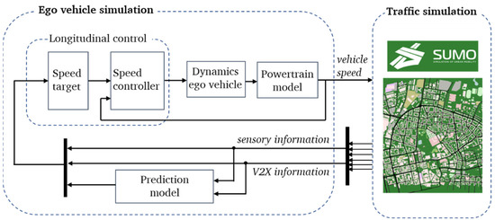
Figure 1.
Co-simulation environment consisting of an ego vehicle simulation and a microscopic traffic simulation.
3.1. Traffic Environment
The traffic environment in which longitudinal controllers are tested plays a significant role for the assessment of the performance of the control. In this section, the microscopic traffic simulator and the description and validation of the traffic model based on real driving data are presented.
3.1.1. Microscopic Traffic Simulator
The traffic simulation used is based on a microscopic traffic model built up in SUMO (Simulation of Urban Mobility) [7]. SUMO is an open source tool for time-discrete and space-continuous simulations of a multi-modal traffic. As a microscopic traffic simulator, SUMO models the behavior of every vehicle individually based on predefined routes, a vehicle type and car-following and lane-changing models. In comparison to macroscopic modeling approaches and transport system models, it does not focus on an extensive demand and supply modeling, but on the simulation of individual vehicles. For this work, a model of the city center of Darmstadt, Germany is derived which is shown in Figure 2. The model consists of a complex road network and a multitude of Traffic Light Systems (TLS). The original 2-dimensional road network is extended with an elevation profile shown in Figure 2b which is derived from a digital topology map based on the 2000 Shuttle Radar Topography Mission [29]. The integration of the elevation leads to grade resistance for the vehicle that affects the respective traction demand and hence the energy consumption of the vehicle.
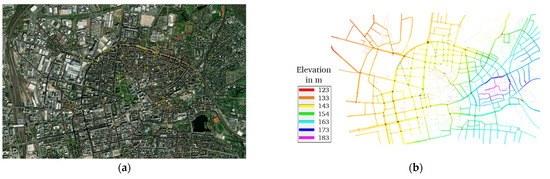
Figure 2.
The modeled area of the city center of Darmstadt, Germany is shown in (a). The integrated elevation profile is shown in (b).
The traffic simulation also contains a model of the simulated traffic fleet. In a microscopic modeling approach, every traffic vehicle is explicitly modeled and is generally characterized by a predefined route and the chosen car-following and lane-changing models. In order to derive a realistic traffic environment, both the car-following model and the macroscopic traffic flows are validated with real driving data which is discussed in the following sections.
3.1.2. Car-Following Modeling Approach
In the co-simulation, the ego vehicle with the proposed control algorithm interacts with other traffic vehicles that are controlled by a microscopic car-following model. According to [30], car-following models can be classified into Gazis-Herman-Rothery models, safety-distance models and psychophysical car-following models. A well-known representative of the first category is the stimulus-response model by GM [31]. Safety-distance car-following models are often based on the Gipps model [32] which always maintains safe distances between ego and leader vehicles. An enhancement to the Gipps model was made within the Krauss model [33], which is the default car-following model used in SUMO. In this work, the Extended Intelligent Driver Model (EIDM) [34] is used which tries to replicate the behavior of a Human-Driven Vehicle (HDV). The model is generally based on the Intelligent Driver Model [35] which calculates the vehicle acceleration with the maximum acceleration and the ratio between the current speed and desired speed as well as the ratio between the desired distance to a leading vehicle and the actual distance .
In Equation (1), denotes the acceleration exponent, a model parameter which is left at its default value in SUMO of . The desired distance is a function of the current speeds of ego and leading vehicle and and further model parameters for the minimum vehicle distance , the desired time headway and the desired deceleration .
In the EIDM, several extensions to the original IDM are combined trying for instance to achieve more realistic gaps between vehicles, to simulate human driver behavior by introducing a reaction time and driver imperfections or to replicate more realistic drive off trajectories. For a more detailed description of the model extensions and their origins, refer to [34].
As can be seen from Equations (1) and (2), the car-following model introduces several model parameters that define the characteristics of a specific driver. In order to yield a realistic traffic environment in which usually many different drivers and vehicles are present, some of the parameters of the EIDM model as well as some vehicle parameters are drawn from normal distributions for every traffic vehicle type in the simulation. A pool of 300 vehicle/driver combinations for passenger cars, buses and trucks is created, respectively. Looking at the main equations of the car-following model, the maximum acceleration, desired deceleration, the desired minimum time headway are the key parameters to define a specific driving style in the model. Additionally, a speed factor is introduced as shown in Equation (3) that is multiplied with the momentary lane speed limit to yield the desired velocity of the driver.
Additionally, the vehicle lengths and emergency decelerations are varied across the traffic vehicle fleet.
3.1.3. Validation of the Car-Following Model
In order to assess the traffic model, real driving data are recorded with a company car that was equipped with a Vector GL2000 data logger. Amongst other signals, the GPS information and velocity/acceleration data are recorded for every trip. The driving data are filtered to only cover the area of Darmstadt that is simulated in SUMO. The filtered dataset contains 470 km of driving data that was recorded with different drivers to yield a wide range of driving styles. To compare the real driving data with the simulated traffic, a driving profile with respect to the occurrence frequencies of vehicle speed and longitudinal acceleration is aggregated for the real driving data and the simulation data, respectively. A number of statistical assessment metrics are then defined for a quantitative comparison. To analyze how well the car-following model reproduces typical acceleration maneuvers in terms of acceleration magnitude and behavior for different vehicle speeds, the 10% and 90% acceleration quantiles as a function of the vehicle speed are calculated. The Mean Squared Error (MSE) between the quantiles of real driving data and simulation data are then determined. Additionally, some key assessment metrics of the driving profiles such as the mean speed and the percentages of standstill and strong decelerations below −3 m/s2 are taken into account. Figure 3 shows a comparison of the simulated driving profiles with the default model parameters of the EIDM and the optimized parameter set. The accelerations in the real driving data mostly stay below 2 m/s2 and decrease towards a vehicle speed of 50 km/h, as this is the dominant vehicle speed limit in the city center. With the default model parameter set, the acceleration of the traffic vehicles tends to be too high compared to the real driving data of the company car, even though buses and trucks are also modeled in the simulation with lower maximum accelerations. A similar conclusion can be drawn for the decelerations which are significantly smaller in the real driving data set. Therefore, both the maximum acceleration and desired deceleration are reduced across all vehicle types to yield a better agreement of real driving data and simulated data with respect to acceleration, as shown in Figure 3b. The mean speed of the driving profile for the default parameter set, on the other hand, is closer to the mean speed of the real driving data. However, there is a higher percentage of driving in areas with a reduced vehicle speed limit of 30 km/h in the simulation, hence the mean speed is generally expected to be lower.
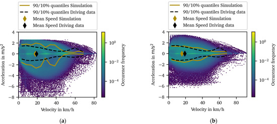
Figure 3.
Aggregated driving profile of the simulated traffic fleet for (a) default model parameters and (b) optimized model parameters. The mean vehicle speeds of the simulated fleet and the measured driving data and the 90% and 10% quantiles of acceleration as a function of vehicle speed are highlighted.
The differences in both model parametrizations with respect to the EIDM model parameters introduced in Section 3.1.1 are summarized in Table 1.

Table 1.
Comparison of the EIDM model parameters and statistical assessment metrics of the resulting driving profiles. The parameters in the default SUMO parametrization are scalar values while the optimized parameters are drawn from normal distributions with given means and standard deviations.
As mentioned before, the MSE for both the acceleration and deceleration quantiles are significantly lower with the optimized parameter set (−71% and −82%, respectively). In addition, the percentage of high decelerations below −3 m/s2 is reduced, indicating a smaller number of emergency decelerations when using the optimized parameter set. The percentage of standstill states is similar for both parameter sets and close to the real driving data.
3.1.4. Validation of the Macroscopic Traffic Flows
Besides the validation of the car-following model that describes the behavior of individual vehicles, the traffic simulation is also validated on a macroscopic level. The goal of the validation is not to derive an exact supply and demand model of the city, but to create a realistic environment for the ego vehicle in terms of traffic density, number of surrounding vehicles and so forth. Generally, the traffic can be described on a macroscopic level by the traffic density or traffic flow at different road segments or junctions. In this work, data from the central traffic management system of Darmstadt is used for validation. The data are publicly available and comprise traffic counts at multiple junctions with traffic lights for different times of day and weekdays [36]. The data of 10 junctions across the city center, as shown in Figure 4a, are processed into total traffic flows of all incoming lanes. Since the traffic flow is varying strongly across different times of the day, two models are derived for a weekday during both rush hour with denser traffic and during an off-peak period with less volume of traffic. This poses different challenges to the prediction of vehicle speeds and an efficient longitudinal control. A detailed description of the vehicle speed prediction model is given in Section 5.
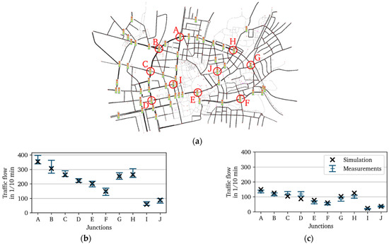
Figure 4.
Cumulative traffic flows at several junctions displayed in (a) in the simulation and from measurement data. The traffic flows are shown during (b) rush hour and during (c) off-peak period. The error bars denote the standard deviations of the traffic flow measurements over the weekdays of one week.
In contrast to more complex demand modeling approaches for transport systems, we use the tools available in SUMO for a simple and efficient generation of traffic demand, since we do not intend to accurately model the traffic demand and supply for the scope of our work. A multitude of routes is first defined for the traffic with the SUMO-internal OSM Web Wizard tool, which generates a traffic demand based on a probability distribution influenced by two parameters, the Through Traffic Factor and the Count parameter. The former defines the likeliness of routes starting and ending at the boundary of the traffic network, and the latter describes how many vehicles are generated per hour and lane-kilometer. The departure times and distribution of vehicles on the routes are adapted afterwards to show a high agreement with the aggregated real traffic flows at every junction. In order to create representative traffic flows for validation based on the traffic data, the traffic flow at a specific junction is obtained for a time period of one hour and over 5 weekdays for one week. Thus, the standard deviation indicates the variation of the traffic flow on different weekdays. As shown in Figure 4b,c, almost all of the simulated traffic flows are within the standard deviation across different days of the week. The results do not necessarily prove a comprehensive validation of the real and simulated traffic demand, but indicate that there is a good agreement with the investigated traffic flows across the traffic network.
3.2. Vehicle Model
The vehicle model is coupled with the traffic simulation in order to simulate the behavior of an ego vehicle inside the previously described traffic scenario and to estimate the energy consumption of vehicles with specific, variable powertrain topologies. Even though this work comprises a case study for Battery Electric Vehicles (BEV) only, the general modeling approach provides an efficient way to derive multiple vehicle concepts and ensure a high comparability through the efficiency-based operating strategy. The generic powertrain model shown in the lower part of Figure 5 comprises two energy converters, i.e., an Internal Combustion Engine (ICE) and an Electric Machine (EM) that can both be used to generate tractive force at the wheels. Generally, some parts of the overall powertrain model can be omitted to create specific powertrain topologies, for instance, a BEV by omitting the ICE and additional generator. By dividing the vehicle transmission into the three sub-transmissions for the model, different hybrid powertrain topologies, for example P2 and P3 configurations, can be derived with varying parametrizations of the sub-transmissions. The additional generator allows for the modeling of a serial hybrid mode (ICE-generator–EM-transmission path). The characteristics of the energy converters are modeled based on efficiency maps of the components; the battery, however, is modeled with a constant efficiency. Electric machines with different rated powers are derived from a reference efficiency map of an electric machine [37] that is scaled along the torque axis to a specific rated power, cf. [38].
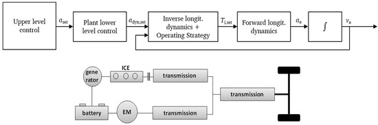
Figure 5.
Overview of the control architecture and the vehicle model which is based on the generic powertrain model shown on the bottom and the simplified lower level control.
Since the focus of this study is on the design and analysis of the upper level longitudinal control which calculates a set acceleration for the vehicle, the lower level control is based on a simplified approach using a first-order lag plant with the lag to approximate its dynamic behavior, which is commonly used when designing an upper level control [39,40].
The longitudinal dynamics of the vehicle are modeled with the driving resistances for aerodynamic drag, rolling resistance and grade resistance.
Here, denotes the effective inertia in longitudinal direction, the aerodynamic drag coefficient, the frontal area of the vehicle, the air density, the rolling resistance coefficient, the gravitational constant and the grade angle of the road.
The tractive force is a function of the operating points of the energy converters (, ) and (, ) which are determined by the inverse longitudinal dynamics and the operating strategy of the vehicle. Here, the Equivalent Consumption Minimization Strategy (ECMS) is used in order to determine the locally optimal operating points with respect to the combined energy consumption which is weighted by the balancing cost factor [41]. The operating strategy chooses the respective optimal torque split between both energy converters and the optimal gear mode by minimizing the cost function .
Here, denotes the brake specific fuel consumption of the ICE, the lower heating value of the fuel, the efficiencies of the battery and EM. This universal definition of the operating strategy allows for the control of every powertrain concept that can be derived from the powertrain topology. BEV for instance can be covered by omitting the first summand of Equation (7) and only determining the optimal gear mode . In case the BEV only has a fixed speed transmission, the operating points are completely predetermined by the vehicle longitudinal acceleration and speed.
4. Control Approach
The main goal of the proposed control approach for the upper level control is to achieve a higher efficiency in terms of vehicle energy consumption in city driving situations through a more anticipatory driving while only increasing the trip time as little as possible. The control approach is also expected to lead to a smoother speed trajectory and therefore increase the driving comfort. Having the ability to predict the behavior of other relevant traffic participants or traffic infrastructure and adjust the own control accordingly is a key property of an efficient driving style of a human driver, for instance, reacting early when upcoming traffic jams or changes in upcoming traffic signals are expected. With the assumption made in this work that a big variety of V2X-based information is available to the ego vehicle, this information can be used to extend the conventional speed and headway control modes of ACC. Generally, there exist multiple technological solutions for V2X communication. A comprehensive survey for V2X technologies is given in [42]. For example, the communication can be based on 5G technology or Visible Light-Communication (VLC). However, for the scope of this study, ideal communication information is assumed. The additional V2X information is used both in free-driving situations when there is no leading vehicle present to reduce stop time at red traffic lights as well as to predict the speeds of both a leading vehicle and the ego vehicle itself over a short prediction horizon for a more anticipatory reaction to the leading vehicle. An overview of the control approach is shown in Figure 6.
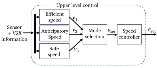
Figure 6.
Framework of the upper level longitudinal control.
The efficient speed control mode here corresponds to the free-driving speed control and the safe speed is a reformulation of the conventional headway control mode of ACC. The additionally introduced anticipatory speed mode uses information from the predicted leader and ego speed to calculate an anticipatory speed target. The mode selection then chooses the smallest, i.e., the safest of the three speed targets and a conventional linear feedback speed controller tracks the chosen speed target. As a side note, building up on the conventional ACC control scheme accommodates for a safety-by-design approach, in which the extensions to the control approach only have a limited, ideally insignificant effect on the safety of the control when the V2X information has a low quality, is corrupted or the prediction is bad. In cases when the V2X-based control decisions would lead to potentially unsafe vehicle states, the minimum-based mode selection always ensures a safe speed target by using the safe speed mode as a fallback level.
For the efficient speed target , the approach of a predictive speed target from [26] is integrated into the framework that incorporates the signal schedule of the next TLS in order to calculate a cruise speed that ideally avoids stops at red traffic lights. The idea is to find the fastest speed to pass the next traffic light in the next green phase which can be described by Equation (8).
Here, and denote the i-th upcoming red or green timing of the next TLS, respectively. The underlying process is an iterative algorithm with the counter i. At first, the intersection for the first red and green timings (i = 1) is calculated. If the intersection is empty, the second interval for i = 2 is determined and its intersection with the defined lower and upper bounds for the TLS set speed is calculated. This process is repeated until i = 3, and if there is still no feasible speed found, is set to the current lane speed. The constant parameter is introduced in order to reduce unwished decelerations when the vehicle approaches the TLS just before turning green. If the ego vehicle approached the red TLS with a constant speed of , it would arrive at the TLS position exactly when the TLS turns green. However, the other control modes would force the vehicle to stop at the TLS, which is still red, inducing an unwished deceleration until the TLS actually turns green. The cruise speed is then defined to be either the predictive speed target , or if there is no feasible intersection found, the lane speed limit .
The anticipatory speed, as described earlier, uses the information from the neural prediction model presented in Section 5 to define a predictive speed target. The general idea is to follow the mean of the predicted leader speed trajectory to achieve the desired anticipatory driving, but also to dampen high oscillations that might occur in the speed trajectory of an aggressive leader. If there is no leading vehicle detected, the speed is set to the mean of the predicted ego speed trajectory instead.
Here, N denotes the number of predicted timesteps and the predicted speeds from the prediction model. By switching to ego speed when there is no leader ahead, the vehicle can not only achieve an anticipatory driving with respect to the expected leader trajectory, but also to its own expected trajectory, reacting, for example, to expected stops at red traffic lights or expected acceleration or deceleration due to an upcoming change of the lane speed limit. Moreover, a lower bound of km/h is defined to ensure the control switches to the headway-based safe speed control mode when coming to a stop.
The third control mode calculates the safe speed based on a common headway control law as a function of the error between the desired and actual headway and the speed difference between leader and ego vehicle [24].
In Equation (11), represents the desired spacing at , the desired time gap and and two controller parameters. The control mode is intended to deal with vehicle states at low distances to leading vehicles or red traffic lights, but can also be considered as a fallback mode when the anticipatory control mode estimates a safety-critical speed target due to a wrong prediction.
As mentioned before, the mode selection chooses the smallest of the three speed targets to always ensure a safe operation of the vehicle. However, the anticipatory speed target needs to be adapted for the selection process. In situations when the distance to a leading vehicle is large, but the prediction model, for instance, estimates a deceleration of the leader, hence is smaller than , it is desired to rather close the gap to the leading vehicle in efficient speed mode before reacting to the predicted leader behavior. Therefore, an adapted speed target is defined for the selection process as a function of the current distance and the ego vehicle speed.
The selection can then mathematically be described by the following equations with .
Note that the whole control approach can be reduced to a conventional ACC law by omitting the anticipatory control mode and the calculation of , i.e., . This reduced formulation acts as a reference control in this work. Since the individual parametrization of both control approaches is identical, a high comparability is ensured.
5. Training and Analysis of the Prediction Model
5.1. Model Definition
The prediction model used in this work gives an estimation of the expected speed trajectories of the leading vehicle and the ego vehicle itself. Note that in this context, upcoming red traffic lights are also considered as ‘virtual’ leading vehicles with , hence the prediction model needs to be able to predict those for a desired early reaction from the longitudinal control. Since the leading vehicle changes frequently in a complex urban traffic situation, the leading vehicle’s trajectory might contain discontinuities and is dependent on many variables such as surrounding traffic, the road network and traffic infrastructure. A conventional speed estimator based on a car-following model could not model the discontinuities of changing leading vehicle and virtual TLS vehicle which is required for a proper anticipatory set speed for the longitudinal control. Moreover, other studies have shown that simple neural network-based approaches can already achieve a higher prediction performance [14].
To deal with this complex prediction task, a supervised learning-based approach is proposed in this work which builds up on a recurrent neural network architecture and a large amount of simulated data collected from the co-simulation environment. A multitude of signals from in-vehicle sensor information as well as V2V- and V2I-based communication , …, over a constant lookback horizon n are used as features for the model. An overview of the features is given in Table 2.
Table 2.
Overview of the complete feature set for the prediction model.
Besides the key sensor-based features such as speeds and accelerations of both vehicles, the feature set also includes information, for instance, about state and program of the TLS or information about upcoming changes in the lane speed limit to accurately predict the behavior of both vehicles. The benefit of all these features for the prediction task remains to be evaluated at this point and is further analyzed in Section 5.2. The chosen definitions lead to a sequence-to-sequence regression modeling approach for the leader speed trajectory , …, and ego speed trajectory , …, . The recurrent neural network as shown in Figure 7 is arranged in an encoder–decoder architecture, a layout for a neural network which was first introduced in [43] for statistical machine translation. The complete neural network here comprises of three hidden layers, which process the information of the feature sequences and give an estimation of the speed trajectories over a later defined prediction horizon.
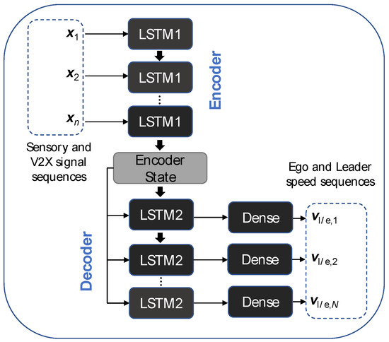
Figure 7.
Architecture of the neural prediction model.
The features are first processed in the encoder in a recurrent LSTM layer (LSTM1). The structure of a single LSTM layer can be described by the following set of equations.
Here, f, i and o denote the input, output and forget gate activation vectors, respectively, c and h the cell state and hidden state vectors, W, U and b the weight matrices and bias vectors and f the nonlinear activation functions. The final hidden state of the encoder is referred to as the encoder state which has encoded all the relevant temporal information of the input sequences in a fixed length vector. It is then used as input for every time step of the LSTM layer of the decoder (LSTM2). Additionally, the final hidden and cell states of the encoder are used as initial values for the hidden and cell state of the decoder to preserve the information encoded in the cell state. The hidden state sequence of the decoder is processed further in a subsequent fully-connected (dense) layer with a Rectified Linear Unit (ReLU) activation and mapped onto the two output sequences of leader and ego speed with a linear activation.
For this work, the lookback and prediction horizon lengths are equally set to to cover a prediction horizon length which is large enough to estimate the behavior of ego and leader vehicles in a meaningful way, but also limit the expected error occurring at larger horizons due to stochastic effects and a limited amount of information in the features.
5.2. Model Training Process
For training of the presented model, a large dataset containing all features from Table 2 is used. The dataset is collected on 84 different routes throughout the modeled road network, every route is simulated six times at different start times and for both the rush hour and off-peak traffic models presented in Section 3.1.3. The total dataset thereby contains 134 h of driving time and 2925 km of driven distance, covering many different traffic situations different leading vehicles with their respective car-following behavior. The dataset is then normalized to [0, 1] in pre-processing to shrink all features values to the same magnitude.
In general, the training can be formulated as an optimization problem in which the loss as a function of the trainable variables W, U and b is minimized. The Mean Absolute Error (MAE) over the prediction horizon and both outputs and is chosen as loss metric.
All training processes in this work are conducted in a Tensorflow Keras environment with the Adam algorithm, which currently is one of the state-of-the-art training algorithms [44]. Note that the default value for from the Keras implementation had to be increased by a few magnitudes for numerical stability of the optimization. The training runs for 500 epochs which has shown to be a robust number for a convergence of the validation loss. In order to find the optimal size of the neural network and the best feature set, a two-stage model selection process is derived which is presented in Figure 8.
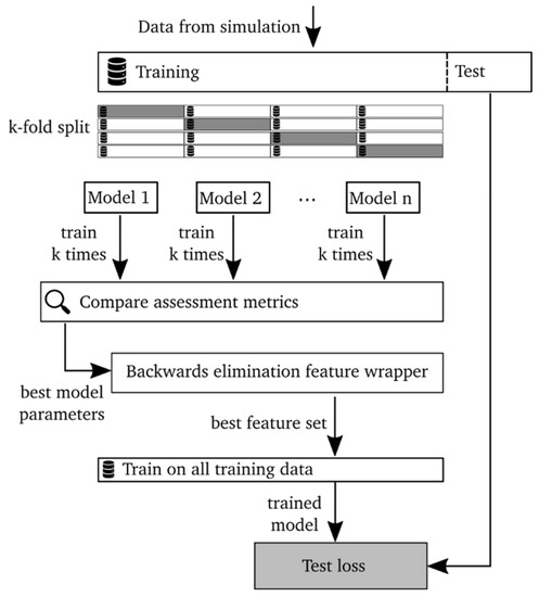
Figure 8.
Workflow of the two-stage model selection process. At the first stage, the main neural network parameters are determined and at the second stage, the best set of features is determined through a backwards elimination feature wrapper method. Both stages use k-fold validation for the training and validation data set.
In the first stage, the optimal network size, i.e., the size of the LSTM and dense layers, is determined. At first, 12 of the 84 routes are split into a test data set that is later used for the final assessment of the model. With the remaining training data, a k-fold validation is conducted, splitting the data up in training and validation data with each different fold using a different part of the data as validation data. Every model is then trained k times and the respective mean of the assessment metrics is used for comparison. In this work, the mean difference between the validation loss and training loss is used together with the commonly used validation loss to assess the individual models. A large difference between validation and training losses can be a sign of a too complex model that tends to overfit on the training data.
In the second stage, a feature wrapper method is applied to analyze the benefit of the features for the prediction quality and to find the best set of features. Feature wrapper methods are greedy search strategies to find an optimal subset of the feature space which achieves a higher performance for the given task. Generally, two main strategies are often distinguished, i.e., forward selection and backwards elimination [45]. Since the total feature number defined for the prediction problem here is rather small and all features are engineered to contain potentially useful information for the prediction, a backwards elimination wrapper is applied here to analyze whether all defined features have a positive effect on the prediction accuracy. In the backwards elimination wrapper implemented here, a model is first trained with the full set of p features. Subsequently, p models with p - 1 features are trained, respectively. The model with the best performance, i.e., lowest validation loss, is compared with . If the best model has a better performance, the algorithm continues, training p - 1 models with p - 2 features, and so on.
Ultimately, a model with the identified optimal size and feature set is trained with the complete training data and assessed on the test data. The results of one model selection process are summarized in Figure 9.
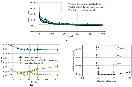
Figure 9.
Results of the model selection process. In (a), the training and validation losses for the selected net size are displayed. The model assessment metrics as a function of net size are shown in (b) and the results of the feature wrapping subprocess are shown in (c).
The results for different net sizes are shown in Figure 9b. The validation loss decreases with larger net sizes until it converges towards a constant level from = 48 onwards. For larger net sizes, there is no improvement on the validation data while at the same time, the difference between validation loss and loss increases, indicating overfitting on the training data. Thus, a net size of is identified to be optimal for the given data. The results of the feature wrapper are shown in Figure 9c. There are a few feature subsets that achieve a lower validation loss on the data, of which the subset without the indicator light of leading vehicle feature is identified to have the lowest validation loss. Dropping even more features results in larger validation losses. The three features that decrease the performance of the prediction model most when left out are the duration until next TLS phase switch , the distance to TLS and the phase of the next TLS , i.e., three V2X-based features. This proves the benefit of using V2X information for the prediction of vehicle speeds.
In order to further analyze the influence of the V2X features on the prediction accuracy, the identified best model with V2X features, a model with only in-vehicle sensor-based features and a naive model which uses a constant acceleration assumption for the prediction are compared.
The test data errors as a function of the timesteps of the prediction horizon for every model are shown in Figure 10.
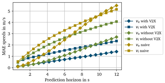
Figure 10.
Comparison of the prediction errors of ego and leader speed and on the test data for the models with V2X features, without V2X features and a naive model with a constant acceleration assumption.
Generally, the speed of the ego vehicle can be predicted with lower errors than the leader speed because it is subject to leader changes due to turning processes or cut-in maneuvers. The mean loss of ego speed at the end of the prediction horizon (t = 12 s) of the V2X-based model is 47% lower compared to the model without V2X features and 72% lower compared to the naive model. For the leader speed, a similar tendency is identified (−42% and −57%). Therefore, a significant benefit in using the V2X information for the prediction task can be stated. When comparing the results to other studies, the differences in the underlying training and test data must be taken into account. However, a MAE of approximately 2.2 m/s for the prediction of leader speed at 10 s is reported in [17] for an enhanced Gaussian Process. Hence, this approach leads to a very similar performance of the prediction model assuming a comparable test data set. In [16], both a naive constant acceleration estimator and an LSTM-based approach are compared for the prediction of ego vehicle speed. The RMSE for the naive and LSTM-based approaches in this study are approximately 5.3 m/s and 1.8 m/s, respectively. Both values are in the same range as for the proposed approach here.
6. Simulative Experiments
6.1. Simulative Case Study
To analyze the behavior of the proposed longitudinal control approach Cp in the presented simulation environment, a number of routes throughout the traffic net and different BEV with varying powertrain specifications are defined. In this study, 10 routes shown in Figure 11 with 6 different starting times are chosen which leads to a total amount of 217 driven km.
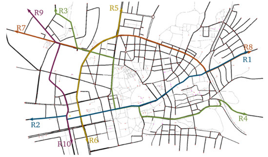
Figure 11.
Test routes for the simulative experiments.
The resulting energy consumptions and the mean vehicle speeds, which are often conflicting objectives, are selected as performance indicators. Additionally, the Root Mean Square (RMS) of the longitudinal jerk is analyzed as an indicator for driving comfort, however driving comfort is generally highly subjective and cannot be fully assessed with this single metric. For comparison, a conventional car-following approach Cref with speed and headway control modes is derived from the architecture shown in Figure 6. As mentioned earlier, both controllers are equally parametrized for a high comparability. Three different vehicles are specified, i.e., three BEV with varying rated powers of the EM and varying transmissions, to assess the robustness of the results towards vehicles with different specifications. A transmission ratio of i = 7 combined with the EM characteristics results in a maximum possible vehicle speed of 160 km/h. Hence, the corresponding operating points in this city driving scenario are rather located in the lower EM speed range. A summary of the key vehicle parameters is given in Table 3. The parameters of the BEV-1 are loosely based on a VW ID.3 powertrain. By also analyzing the two-speed BEV, more insight into the effects of different operating points on the vehicle energy demand can be gained.
Table 3.
Vehicles derived from the powertrain architecture for the experiments.
6.2. Results
The results of the previously defined case study are summarized in this section. At first, the longitudinal control is discussed for one of the defined routes in more detail. The estimated vehicle speed trajectories over the course of Route 5 are shown in Figure 12. As mentioned before, the leader speed trajectory contains some discontinuities due to the switching of detected leading objects (vehicles/TLS) which makes the prediction much more challenging. However, the general trends show a good agreement with the actual trajectory. In particular, the starts of deceleration maneuvers are often correctly predicted. With respect to the ego speed, the prediction model incorrectly anticipates a deceleration twice at t = 150 s and t = 250 s, but otherwise achieves a high prediction accuracy along the route.
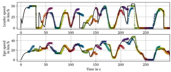
Figure 12.
Comparison of predicted (colored) and actual (black) ego and leader speeds on Route 5.
In Figure 13, exemplary results for vehicle speed, acceleration and jerk as a function of the driven distance on Route 5 are shown for Cp and Cref. Generally, Cp operates 44% of the time in the anticipatory control mode and 30% in efficient speed mode and only switches into safe speed mode when the headway to the leader is too small. In the first section of the route, several stops at junctions that occur with the reference control Cref can be avoided by first tracking a set speed below the lane speed limit of 50 km/h and then switching into anticipatory control to track the predicted mean speed of the leader’s trajectory. The trip time up to a driving distance of 1500 m is nearly identical, although the accelerations with Cp overall are considerably lower. On this single exemplary route, the BEV-1 with Cp has a significantly lower consumption of 12.77 kWh/km in comparison to 15.59 kWh/km with Cref. This reduction is mainly caused by the less frequent braking, lowering the overall breaking losses. Even though the BEV are able to recuperate some of the kinetic energy when braking, a significant percentage of the energy is lost during the conversion of energy in the electric machine.
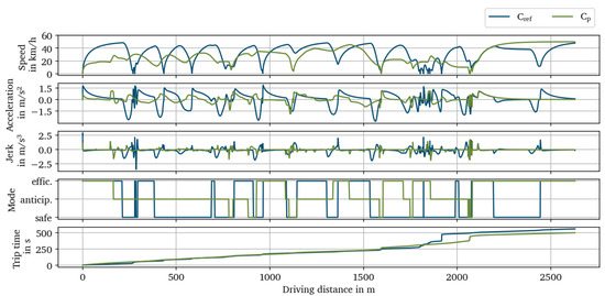
Figure 13.
Exemplary results for Cref and Cp on Route 5.
When analyzing the performance indicators on the different routes individually, there is a big variance in the differences between Cp and Cref. The results are shown in Figure 14 for both the rush hour and the off-peak period traffic models of BEV-1. In general, Cp achieves a reduction in the energy consumption across all routes and traffic models of 3.3–23.2% while lowering the mean speed up to 20.5%. However, there are several routes, for instance, R9 during rush hour or R3 during the off-peak period, in which using Cp results in a significant reduction in energy consumption while sustaining the same mean speed. Regarding the jerk, the more anticipatory driving with Cp reduces the RMS of jerk across all routes up to 28.2%.
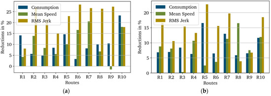
Figure 14.
Reductions of performance indicators with the proposed control Cp compared to the reference Cref for BEV-1. The results are shown for (a) the rush hour and (b) the off-peak period.
A summary of all performance indicators across the three investigated vehicles and both traffic models is given in Table 4. It is shown that the mean speeds during rush hour are always lower than during the off-peak period due to the higher traffic density. At the same time, the energy consumptions in the off-peak period are always lower. This indicates that the consumption is dominated by the losses for decelerating and accelerating more frequently, losses due to aerodynamic drag at a higher mean speed only play a minor role. Both of the two-speed BEV have a lower energy consumption than the fixed-speed BEV, showing the benefit of a shiftable transmission for BEV. For BEV-2, the difference is higher, also because of the smaller EM resulting in operating points with higher efficiency. However, even the BEV-3 with a larger EM power than BEV-1 achieves a smaller consumption due to the additional degree of freedom in the operating strategy of choosing one of the two speeds. When averaging over all analyzed routes, traffic models and vehicles, Cp leads to a mean reduction in the energy consumption of 6.7%.
Table 4.
Summary of the performance indicators.
7. Conclusions
This study proposes an anticipatory longitudinal control approach for variable vehicles in urban traffic. The control utilizes the estimated speed trajectories of ego and leader vehicle to accomplish an ecological driving and reduce the energy consumption of the vehicle. In order to achieve a good prediction, a neural prediction model based on a recurrent encoder–decoder structure is trained with data from both in-vehicle sensors and V2X communication. It could be shown that the model achieves a similar performance compared to other methodical approaches and that the V2X features highly improve the prediction accuracy of the model. The co-simulation environment created allows for both the collection of the training data and the efficient assessment of different vehicles. The validation and adaption of the traffic models with real driving and traffic data ensures a realistic traffic scenario and is recommended for further studies in which representative vehicle energy consumptions are calculated in simulative environments. The scope of this study was applied to a case study with three different BEV for which a significant reduction of vehicle consumption by 6.7% and a considerable reduction of the jerk could be proven at the cost of a slight increase in trip time, compared to a reference ACC control. This can increase the range of electric vehicles which is often a barrier when purchasing an electric vehicle. On the other hand, the capacity of the battery could be reduced for the same range which lowers the ecological impact of the vehicle during production, as the battery production is very energy intensive. The results and performance of the prediction model must be seen under the assumption of ideal V2X information. For a real-world application, the influence of noisy or incomplete V2X information on the performance must be further analyzed. The analysis of the prediction model performance showed a strong improvement in prediction accuracy through the V2X information. Hence, this information has to be made available to the vehicle fleet in order to achieve the improvement in energy demand reported in this study. Future investigations can be made for additional vehicle concepts such as HEV or the CityBot with four in-wheel motors and optimizing the parametrization of the control. The scope of this article was to analyze the benefits of the integrated V2X information and prediction model compared to a conventional control law. Combining the approach with an optimization-based control approach such as MPC may further increase the performance of the control. Furthermore, the safety of new proposed control strategies that incorporate additional data and learning systems need to be considered in early development stages. Therefore, continuing studies are planned to analyze the effect of incomplete or corrupted V2X data, which is expected to decrease the prediction accuracy of the neural prediction model, but only have a small impact on the safety of the control through the safety-by-design aspect of the proposed control approach.
Author Contributions
Conceptualization, T.E.; methodology, T.E. and P.H.; software, T.E.; validation, T.E.; formal analysis, T.E.; writing—original draft preparation, T.E. and P.H..; writing—review and editing, T.E., P.H. and S.R.; visualization, T.E.; supervision, S.R.; project administration, S.R. All authors have read and agreed to the published version of the manuscript.
Funding
The Campus FreeCity project is funded with a total of 10.9 million euros by the German Federal Ministry for Digital and Transport (BMDV), grant number 45KI15I091.

Data Availability Statement
Not applicable.
Conflicts of Interest
The authors declare no conflict of interest.
References
- European Environment Agency. Grennhouse Gas Emissions from Transport in Europe. Available online: https://www.eea.europa.eu/ims/greenhouse-gas-emissions-from-transport (accessed on 1 December 2022).
- Bernard, M.R.; Hall, D.; Lutsey, N. Update on Electric Vehicle Uptake in European cities, Hungary, Budapest. 2021. Available online: https://theicct.org/publication/update-on-electric-vehicle-uptake-in-european-cities/ (accessed on 1 December 2022).
- Donkers, A.; Yang, D.; Viktorović, M. Influence of driving style, infrastructure, weather and traffic on electric vehicle performance. Transportation Research Part D Transp. Environ. 2020, 88, 102569. [Google Scholar] [CrossRef]
- Boban, M.; Kousaridas, A.; Manolakis, K.; Eichinger, J.; Xu, W. Use Cases, Requirements, and Design Considerations for 5G V2X. arXiv 2017, arXiv:1712.01754. [Google Scholar] [CrossRef]
- Katsaros, K.; Kernchen, R.; Dianati, M.; Rieck, D.; Zinoviou, C. Application of vehicular communications for improving the efficiency of traffic in urban areas. Wirel. Commun. Mob. Comput. 2011, 11, 1657–1667. [Google Scholar] [CrossRef]
- Watzenig, D.; Horn, M. Automated Driving: Safer and More Efficient Future Driving; Springer International Publishing: Cham, Switzerland, 2017. [Google Scholar] [CrossRef]
- Lopez, P.A.; Behrisch, M.; Bieker-Walz, L.; Erdmann, J.; Flötteröd, Y.P.; Hilbrich, R.; Lücken, L.; Rummel, J.; Wagner, P.; Wießner, E. Microscopic Traffic Simulation using SUMO. In 21st IEEE International Conference on Intelligent Transportation Systems; IEEE: Piscataway, NJ, USA, 2018; pp. 2575–2582. [Google Scholar]
- Gora, P.; Katrakazas, C.; Drabicki, A.; Islam, F.; Ostaszewski, P. Microscopic traffic simulation models for connected and automated vehicles (CAVs)–state-of-the-art. Procedia Comput. Sci. 2020, 170, 474–481. [Google Scholar] [CrossRef]
- Nowack, B. Campus FreeCity: Living Lab to Explore a Networked Fleet of Modular Robotic Vehicles. Available online: https://www.campusfreecity.de/ (accessed on 1 December 2022).
- Pan, C.; Huang, A.; Chen, L.; Cai, Y.; Chen, L.; Liang, J.; Zhou, W. A review of the development trend of adaptive cruise control for ecological driving. Proc. Inst. Mech. Eng. Part D J. Automob. Eng. 2022, 236, 1931–1948. [Google Scholar] [CrossRef]
- Desjardins, C.; Chaib-draa, B. Cooperative Adaptive Cruise Control: A Reinforcement Learning Approach. IEEE Trans. Intell. Transport. Syst. 2011, 12, 1248–1260. [Google Scholar] [CrossRef]
- Liu, Y.; Zhou, A.; Wang, Y.; Peeta, S. Proactive Longitudinal Control of Connected and Autonomous Vehicles with Lane-Change Assistance for Human-Driven Vehicles. In 2021 IEEE International Intelligent Transportation Systems Conference (ITSC); IEEE: Piscataway, NJ, USA, 2021. [Google Scholar]
- Lin, Y.; McPhee, J.; Azad, N.L. Comparison of Deep Reinforcement Learning and Model Predictive Control for Adaptive Cruise Control. arXiv 2019, arXiv:1910.12047. [Google Scholar] [CrossRef]
- Lefevre, S.; Sun, C.; Bajcsy, R.; Laugier, C. Comparison of Parametric and Non-Parametric Approaches for Vehicle Speed Prediction. In 2014 American Control Conference (ACC 2014), Portland, Oregon, USA, 4–6 June 2014; IEEE: Piscataway, NJ, USA, 2014; pp. 3494–3499. [Google Scholar] [CrossRef]
- Mozaffari, A.; Vajedi, M.; Azad, N.L. A robust safety-oriented autonomous cruise control scheme for electric vehicles based on model predictive control and online sequential extreme learning machine with a hyper-level fault tolerance-based supervisor. Neurocomputing 2015, 151, 845–856. [Google Scholar] [CrossRef]
- Yeon, K.; Min, K.; Shin, J.; Sunwoo, M.; Han, M. Ego-Vehicle Speed Prediction Using a Long Short-Term Memory Based Recurrent Neural Network. Int. J. Automot. Technol. 2019, 20, 713–722. [Google Scholar] [CrossRef]
- Morlock, F.; Sawodny, O. An economic model predictive cruise controller for electric vehicles using Gaussian Process prediction. IFAC-Pap. 2018, 51, 876–881. [Google Scholar] [CrossRef]
- Altche, F.; de La Fortelle, A. An LSTM Network for Highway Trajectory Prediction. In Proceedings of the 20th International Conference on Intelligent Transportation Systems: Mielparque Yokohama in Yokohama, Kanagawa, Japan, 16–19 October 2017. [Google Scholar]
- Jiang, B.; Fei, Y. Traffic and vehicle speed prediction with neural network and Hidden Markov model in vehicular networks. In 2015 IEEE Intelligent Vehicles Symposium (IV), Seoul, Republic of Korea, 28 June–1 July 2015; IEEE/Institute of Electrical and Electronics Engineers Incorporated: Piscataway, NJ, USA, 2015; pp. 1082–1087. [Google Scholar]
- Park, S.H.; Kim, B.; Kang, C.M.; Chung, C.C.; Choi, J.W. Sequence-to-Sequence Prediction of Vehicle Trajectory via LSTM Encoder-Decoder Architecture, 2018. In 2018 IEEE Intelligent Vehicles Symposium (IV); IEEE: Piscataway, NJ, USA, 2018; pp. 1672–1678. [Google Scholar] [CrossRef]
- Houenou, A.; Bonnifait, P.; Cherfaoui, V.; Yao, W. Vehicle Trajectory Prediction Based on Motion Model and Maneuver Recognition. In 2013 IEEE/RSJ International Conference on Intelligent Robots and Systems; IEEE: Piscataway, NJ, USA, 2013; pp. 4363–4369. [Google Scholar]
- Deo, N.; Trivedi, M.M. Convolutional Social Pooling for Vehicle Trajectory Prediction. In 2018 IEEE/CVF Conference on Computer Vision and Pattern Recognition Workshops, CVPRW 2018, Salt Lake, UT, USA, 18–22 June 2018; IEEE: Piscataway, NJ, USA, 2018; pp. 1549–15498. [Google Scholar]
- Eichenlaub, T.; Rinderknecht, S. Anticipatory Longitudinal Vehicle Control using a LSTM Prediction Model. In 21 IEEE International Intelligent Transportation Systems Conference (ITSC); IEEE: Piscataway, NJ, USA, 2021; pp. 447–452. [Google Scholar] [CrossRef]
- Winner, H.; Hakuli, S.; Lotz, F.; Singer, C. Handbuch Fahrerassistenzsysteme; Springer Fachmedien Wiesbaden: Wiesbaden, Germany, 2015. [Google Scholar]
- Zhao, Z.; Xun, J.; Wan, X.; Yu, R. MPC Based Hybrid Electric Vehicles Energy Management Strategy. IFAC-PapersOnLine 2021, 54, 370–375. [Google Scholar] [CrossRef]
- Asadi, B.; Vahidi, A. Predictive Cruise Control: Utilizing Upcoming Traffic Signal Information for Improving Fuel Economy and Reducing Trip Time. IEEE Trans. Contr. Syst. Technol. 2011, 19, 707–714. [Google Scholar] [CrossRef]
- Yoon, Y.; Yi, K. Design of Longitudinal Control for Autonomous Vehicles Based on Interactive Intention Inference of Surrounding Vehicle Behavior Using Long Short-Term Memory; IEEE: Piscataway, NJ, USA, 2021. [Google Scholar]
- Malek, Y.N.; Najib, M.; Bakhouya, M.; Essaaidi, M. Multivariate deep learning approach for electric vehicle speed forecasting. Big Data Min. Anal. 2021, 4, 56–64. [Google Scholar] [CrossRef]
- de Ferranti, J. Viewfinder Panoramas. Available online: http://viewfinderpanoramas.org/dem3.html (accessed on 15 May 2022).
- Ahmed, H.U.; Huang, Y.; Lu, P. A Review of Car-Following Models and Modeling Tools for Human and Autonomous-Ready Driving Behaviors in Micro-Simulation. Smart Cities 2021, 4, 314–335. [Google Scholar] [CrossRef]
- Gazis, D.C.; Herman, R.; Rothery, R.W. Nonlinear Follow-The-Leader Models of Traffic Flow. Oper. Res. 1961, 9, 545–567. [Google Scholar] [CrossRef]
- Gipps, P.G. A behavioural Car-Following Model for Computer Simulation. Transp. Res. Part B Methodol. 1981, 15, 105–111. [Google Scholar] [CrossRef]
- Krauß, S. Microscopic Modeling of Traffic Flow: Investigation of Collision Free Vehicle Dynamics. Ph.D. Thesis, Universität Köln, Köln, Germany, 1998. [Google Scholar]
- Salles, D.; Kaufmann, S.; Reuss, H.-C. Extending the Intelligent Driver Model in SUMO and Verifying the Drive Off Trajectories with Aerial Measurements. In SUMO User Conference 2020; TIB Open Publishing: Hannover, Germany, 2020. [Google Scholar]
- Treiber, M.; Hennecke, A.; Helbing, D. Congested traffic states in empirical observations and microscopic simulations. Phys. Rev. E 2000, 62, 1805–1824. [Google Scholar] [CrossRef]
- Wissenschaftsstadt Darmstadt. Open Traffic Data. Available online: https://datenplattform.darmstadt.de/verkehr/apps/opendata/#/ (accessed on 27 October 2022).
- An, J.; Binder, A. Operation Strategy with Thermal Management of E-Machines in Pure Electric Driving Mode for Twin-Drive-Transmission (DE-REX). In IEEE Vehicle Power and Propulsion Conference (VPPC) 2017; IEEE: Piscataway, NJ, USA, 2017. [Google Scholar]
- Esser, A.; Eichenlaub, T.; Schleiffer, J.E.A. Comparative evaluation of powertrain concepts through an eco-impact optimization framework with real driving data. Optim. Eng. 2021, 22, 1001–1029. [Google Scholar] [CrossRef]
- Huang, J. Vehicle Longitudinal Control. In Handbook of Intelligent Vehicles; Eskandarian, A., Ed.; Springer: London, UK, 2012; pp. 167–190. ISBN 978-0-85729-084-7. [Google Scholar]
- Rajamani, R. Vehicle Dynamics and Control; Mechanical Engineering Series. Springer Science+Business Media, Inc.: New York, NY, USA, 2006. [Google Scholar]
- Paganelli, G.; Delprat, S.; Guerra, T.M.; Rimaux, J.; Santin, J.J. Equivalent consumption minimization strategy for parallel hybrid powertrains. 55th Veh. Technol. Conf. 2022, 4, 2076–2081. [Google Scholar] [CrossRef]
- Alalewi, A.; Dayoub, I.; Cherkaoui, S. On 5G-V2X Use Cases and Enabling Technologies: A Comprehensive Survey. IEEE Access 2021, 9, 107710–107737. [Google Scholar] [CrossRef]
- Cho, K.; van Merrienboer, B.; Gulcehre, C.; Bahdanau, D.; Bougares, F.; Schwenk, H.; Bengio, Y. Learning Phrase Representations using RNN Encoder-Decoder for Statistical Machine Translation. arXiv 2014, arXiv:1406.1078. [Google Scholar] [CrossRef]
- Kingma, D.P.; Ba, J. Adam: A Method for Stochastic Optimization. arXiv 2014, arXiv:1412.6980. [Google Scholar]
- Kohavi, R.; John, G.H. Wrappers for feature subset selection. Artif. Intell. 1997, 97, 273–324. [Google Scholar] [CrossRef]


Disclaimer/Publisher’s Note: The statements, opinions and data contained in all publications are solely those of the individual author(s) and contributor(s) and not of MDPI and/or the editor(s). MDPI and/or the editor(s) disclaim responsibility for any injury to people or property resulting from any ideas, methods, instructions or products referred to in the content. |
© 2022 by the authors. Licensee MDPI, Basel, Switzerland. This article is an open access article distributed under the terms and conditions of the Creative Commons Attribution (CC BY) license (https://creativecommons.org/licenses/by/4.0/).