A Real-Time Energy Consumption Minimization Framework for Electric Vehicles Routing Optimization Based on SARSA Reinforcement Learning

Abstract

A real-time, metadata-driven electric vehicle routing optimization to reduce on-road energy requirements is proposed in this work. The proposed strategy employs the state–action–reward–state–action (SARSA) algorithm to learn the EV’s maximum travel policy as an agent. As a function of the received reward signal, the policy model evaluates the optimal behavior of the agent. Markov chain models (MCMs) are used to estimate the agent’s energy requirements on the road, in which a single Markov step represents the average energy consumption based on practical driving conditions, including driving patterns, road conditions, and restrictions that may apply. A real-time simulation in Python with TensorFlow, NumPy, and Pandas library requirements was run, considering real-life driving data for two EVs trips retrieved from Google’s API. The two trips started at 4.30 p.m. on 11 October 2021, in Los Angeles, California, and Miami, Florida, to reach EV charging stations six miles away from the starting locations. According to simulation results, the proposed AI-based energy minimization framework reduces the energy requirement by 11.04% and 5.72%, respectively. The results yield lower energy consumption compared with Google’s suggested routes and previous work reported in the literature using the DDQN algorithm.

1. Introduction

Transportation electrification has emerged as a pivotal solution to combat climate change by offsetting emissions from the two main contributors to greenhouse gas emissions (GHG): the transportation sector and the power industry. To expedite transportation electrification, governments around the globe have recently adopted progressive policies and supported research to facilitate the fast and reliable integration of millions of electric vehicles (EVs) on the road. Nevertheless, efforts are still needed to increase confidence in EVs as a reliable technology and overcome internal battery energy management concerns. This includes extending the driving range of EVs to reduce range anxiety, which is the fear of running out of power while not finding a charging station. According to [1,2], this resembled a significant obstacle to the large-scale adoption of EVs. This work presents a real-time, metadata-driven, reinforcement learning-based energy consumption minimization strategy that allows EVs to extend their driving range. This is especially during conditions where EV owners are more concerned with the amount of energy required to reach a charging destination than with arrival time. The proposed framework is based on the SARSA, an iterative, on-policy, reinforcement learning algorithm that computes the expected value of a policy considering the explorative behavior of an agent.

Reinforcement learning (RL) is an artificial intelligence technique widely accepted as an efficient tool for solving various scientific problems [3]. In the recent decade, several works in the literature have employed reinforcement learning to perform electric vehicle-related studies, such as in optimal EV routing [4], intelligent EV charging scheduling [5], and powertrain optimization for hybrid and PEVs [6,7]. It is worth mentioning that the study conducted in [4] was successfully performed by the authors of this work based on the DDQN algorithm; therefore, its results will serve as a benchmark for the proposed work. Away from electric vehicles, RL techniques have widely been utilized to perform a wide range of studies in the energy field. Reference [8] proposes residential load management based on RL to effectively design price-based demand response programs to control smart buildings’ loads. Reference [9] utilizes RL to optimize the maintenance scheduling of the power grids. RL was used in [10] to coordinate strategic bidding for power markets, where multidimensional continuous states and action spaces enable the market participants to receive accurate feedback regarding the impact of their bidding decisions. While other studies have deployed RL for robotic control [11,12], cybersecurity of smart grids [13,14], computer systems architecture [15,16], traffic congestion relief and coordination [17,18], and wireless systems and communication networks [19,20], there are still limitations to the use of RL-SARSA in the EV-related research literature. Previous studies have shown the capability of the SARSA algorithm to effectively solve problems ranging from EV charging control [21], demand response in smart grids [22], peer-to-peer energy transactions [23], to hybrid EVs controllers and powertrains [24,25]. More importantly, the EV routing optimization problem is an underexplored research area in a time where range anxiety remains one of the challenges to expanding the EV market [26]. To complement such deficiencies, this work proposes a real-time, metadata-driven RL-SARSA algorithm-based routing optimization to reduce on-road EV energy requirements to extend the drivability range. The proposed approach evaluates Q-values through the state–action–reward–state–action (SARSA) algorithm to train the EV as an agent that independently chooses optimal actions that resemble driving decisions with lower energy requirements. Ultimately, the learning process extends the drivability range of the EV. The driving dynamics of EVs are achieved following the Markov chain model (MCM) to evaluate the energy needs for on-road trips with respect to the proposed framework. The agent’s learning experience is supplemented with real-time metadata provided by Google’s API platform to feed the agent with continuously updated driving information.

The rest of this article is organized as follows: Section 2 shows the primary concepts of RL and MCM utilized with the SARSA algorithm; Section 3 presents the proposed strategy to achieve energy consumption minimization, the metadata extraction process from Google’s API, and the application of the SARSA algorithm; Section 4 shows the experimental results of the proposed strategy for two geographically different trips; and Section 5 concludes the work.

2. Reinforcement Learning

2.1. State–Action–Reward–State–Action (SARSA) Algorithm

State–action–reward–state–action (SARSA) is an artificial intelligence algorithm based on the Markov decision process (MDP). Considered one of the well-established algorithms in the reinforcement learning area of machine learning, SARSA was firstly proposed by Rummery and Niranjan [27] as the “Modified Connectionist Q-Learning MCQL” algorithm. Sutton [28] later suggested the current name SARSA. SARSA and Q-learning are two famous RL algorithms based on temporal difference learning (TD), with a high capability of establishing a learning process that eventually produces successive decision-making steps. Reinforcement learning utilizes the concept of an agent that operates in a given environment to infer a policy, Π, following a set of self-explanatory actions a_i, and states s_i, computed Q-values, and reward signals, R. The agent can only choose a certain action based on its current state, influenced by a positive or negative reward signal established by the learning process. In addition, a discount factor γ is suggested concerning the learning strategy’s design goals. The closer γ gets to unity, the more influence the next reward will have on the current state, and vice versa. Reward signals, therefore, serve as feedback that indicates the possibility of failure or success of the action in relation to the learning process.

The concept of SARSA is that the primary function used to update the Q-value depends on the current state of the agents. The action that the agent chooses “a”, the reward signal “r” that influences the agent to select the proper action, the state “s’” that the agent enters after taking that specific action, and finally, the following action “a’” the agent chooses in its new state. In SARSA, the agent uses the state–value function in conjunction with the epsilon greedy policy to perform exploration and exploitation. Based on the weights of the obtained Q-values, the following process grades the states and estimates their relative strength as follows:

$$V^{\pi }\left(s\right)=\mathbb{E} [{\sum }_{\acute{a}\in A}^{ } \gamma r\left(s,a\right)\mathrm{I} s]$$

(1)

$$Q^{\pi }\left(s,a\right)=\mathbb{E} [{\sum }_{\mathrm{t}}^{ } \gamma r\left(s,a\right)\mathrm{I} s,a]$$

(2)

where A is the set of agent’s actions a_i ∈ A; s_i ∈ S is the set of agent’s states; $Q_i\left(s,a\right)$ and $r_i\left(s,a\right)$ as the corresponding Q-value and reward signal; and $\pi$ as the control policy in the learning process. While Equation (1) defines the state–value relationship, Equation (2) highlights the action–value correlation. The major difference between the two functions lies in whether the agent’s current action is known. As a result, the action–value function is usually utilized to derive the optimal action at each time step. Therefore, Equation (2) could be better rewritten as the Bellman form as follows:

$$Q^{\pi }\left(s,a\right)=r_i\left(s,a\right)+\gamma {\sum }_{\acute{s}\in S}^{ }{P}_i\left(\acute{s }\mathrm{I} s,a\right)Q_i^{\pi }\left(\acute{s},\acute{a}\right)$$

(3)

where P(s’| s, a) is the probability of the agent transitioning between any two consecutive states following a given action, while s’, a’ are the updated state and action. Then, the agent can decide on an optimal action by either feedback obtained by maximizing or minimizing the value function, as follows:

$${\mathsf{\pi }}^{*}\left(\mathrm{s}\right)=\underset{\mathrm{a}}{\mathrm{argmax}} \{r_i\left(s,a\right)+\gamma {\sum }_{\acute{s}\in S}^{ }{P}_i\left(\acute{s }\mathrm{I} s,a\right)Q_i^{\pi }\left(\acute{s},\acute{a}\right) \}$$

(4)

The major goal behind RL is to train the agent with a policy (π) that maximizes reinforcements that influences the agent’s behavior, mapping its states into optimal actions. $\epsilon$-greedy is a methodology for optimal action selections in RL, where the parameter $\epsilon$ $\in \left[0,1\right]$ is defined, and the policy π(s) could be utilized as follows:

$$\pi \left(s\right)=\{\begin{array}{cc}\acute{a}& with probability 1-\epsilon \\ a_r& with probability \epsilon \end{array}$$

(5)

where $\acute{a}$ is the best-obtained action for the state $s$, while $a_r$ is the agent that selects a random action with a probability ε. As one may notice, for each time step, the optimal control policy is achieved by iterative calculations of the action–value matrix Q (s,a). In this work, the $\epsilon$-greedy policy is utilized to decide the optimal control actions for the agent, as it explores a random control action with a probability that increases when the learning experience advances. This point distinguishes the SARSA from the Q-learning algorithm of reinforcement learning. In SARSA, the current and subsequent actions of the agent are all chosen by greedy policy, making it an on-policy. Conversely, in Q-learning, the agent’s following action is not determined by the greedy online policy, making it an off-policy. The SARSA updates the Q-values utilizing the following expression:

$$Q_{t+1}\left(s,a\right)\leftarrow Q_t\left(s,a\right)+\alpha \left\{r_i\left(s,a\right)+\gamma Q_t\left(\acute{s},\acute{a}\right)-Q_t\left(s,a\right)\right\}$$

(6)

where $a$ is the learning rate that has values ∈ [0,1]. As mentioned earlier, the epsilon greedy policy is utilized to determine the agent’s optimal action in Equation (6). As one may notice, this may yield a better exploration strategy but with the drawback of consuming more time, presenting SARSA as a better strategy than Q-learning to obtain optimal values, yet possibly may yield more time to achieve such a purpose. Another significant difference between SARSA and Q-learning is that the SARSA algorithm can obtain a different policy when exploration of the agent may result in hefty penalties. For example, suppose the agent (an EV) navigates near an unreachable position that poses a danger, such as driving toward a lake or a tree next to the side of the road. In that case, even if this is an optimal policy per calculations, it will be dangerous for exploration steps. As a result, SARSA will note this and adopt a policy that keeps the EV away from that side of the road through its drive. In other words, SARSA will find an optimal policy considering the exploration inherited in the policy. A third distinction between the two RL algorithms could be seen from the aspect of the agent’s policy; behavior or learning. For instance, the behavioral approach generates actions because of the agent’s interaction with its surrounding environment. Then, the learning strategy influences the agent to learn through such interactions. For SARSA, both behavioral and learning approaches are equal, while this is not the case for the DDQN algorithm.

Agents can find themselves in an actual instant situation, known as the state, in a given environment, such as a transportation system that has a driver to guide them to their destination. This work assumes an EV to be the agent that learns from its present state to infer its next state by using a strategy that achieves maximal rewards (i.e., minimal energy consumption), known as the learning policy Π. The SARSA algorithm provides artificial learning that determines the agent’s next action. The agent achieves the next reward with each additional step. As a result of this reward, the learning process establishes the new state, s’, with a particular probability of transforming between states. The mapping represents the learning policy and the sequence of actions and states required to achieve any reward is known as the trajectory. Figure 1 provides an illustration of the concept of SARSA-RL utilized in this work.

The pseudo-code of the proposed energy consumption minimization strategy based on SARSA is shown in

Table 1. Pseudo-code of the SARSA algorithm.

SARSA Algorithm

Retrieve the agent’s geocode location. Initialize Q ($s,a$), state ($s$), and the number of iteration k. Calculate$W_i\left(P\right)$, generate$Q_M$. Repeat each step k s.t. k = 1, 2,.…k. Determine optimal action a, depend on Q(s, ·), following ε-greedy policy. Based on action a; observe reward r and next state$\acute{s}$ Determine actioná = arg maxa $Q_t\left(s,a\right)$ $Q_{t+1}\left(s,a\right)\leftarrow Q_t\left(s,a\right)+\alpha \left\{r_i\left(s,a\right)+\gamma Q_t\left(\acute{s},\acute{a}\right)-Q_t\left(s,a\right)\right\}$ $s\leftarrow \acute{s}$ Repeat until$s$is terminal.

. The number of episodes considered in this work is 140, with a maximum of 1000 iterations within each episode. It is worth mentioning that the learning rate is continuously changing with time and is decided as $1/\sqrt{k+2}$, with a sample time of 1 s. The reward signal for moving between states $i \mathrm{and} j$ is estimated as follows:

$$R_j^i=\frac{1}{\frac{E_l\left(i,j\right)}{E_h\left(i,j\right)}}$$

(7)

where $E_l\left(i,j\right)$ and $E_h\left(i,j\right)$ correspond to the best and highest energy requirement obtained in a driving cycle between states $i \mathrm{and} j$, respectively. For the agent to reach an optimal policy is equivalent to converging the obtained Q-value to the Q-values desired for the next time step. For each newly integrated input data at time slot t, the Q-update and its probabilistic information can be expressed as follow:

$$V_{\mathrm{t}}\left(s,\pi \left(s\right)\right)=r_{\pi \left(s\right)}\left(s,\acute{s}\right)+\gamma Q_t\left(\acute{s},\pi \left(\acute{s}\right)\right)$$

(8)

$$\mathbb{E}\left(V_{\mathrm{t}}\right)=Q_t^{*}\left(s,\pi \left(s\right)\right)$$

(9)

$$\mathbb{V}ar\left(V_{\mathrm{t}}\right)={\sigma }_t^2\left(s,\pi \left(s\right)\right)$$

(10)

To fittingly train the estimator, a common loss function is utilized as follows:

$$ℒ{[Q_t\left(s,\pi \left(s\right)\right)\left]=0.5 \right[Q_t\left(s,\pi \left(s\right)\right)-V_{\mathrm{t}}\left(s,\pi \left(s\right)\right)]}^2$$

(11)

$$\mathbb{E}\left(ℒ\left[Q_t\left(s,\pi \left(s\right)\right)\right]\right)=0.5 \{{[Q_t\left(s,\pi \left(s\right)\right)-Q_t^{*}\left(s,\pi \left(s\right)\right)]}^t+{\sigma }_t^2\left(s,\pi \left(s\right)\right)\}$$

(12)

$$\mathbb{V}ar\left(\mathbb{X}\right)=\mathbb{E}\left({\mathbb{X}}^2\right)-\mathbb{E}{(\mathbb{X})}^2$$

(13)

$ℒ$ resembles the loss value to be calculated at the i^th iteration and is an indication of the distance between the obtained Q-values and the Q-values at the next time step. The target value at the i^th iteration, which could be found as follows:

$$g_i\left(s,a\right)=r_i\left(s,a\right)+\gamma {\displaystyle \sum }_{\stackrel{‘}{s}\in S}{P}_i\left(s\prime |s,a\right) Q_i\left(\grave{s},\grave{a};{\theta }_{i-1}\right)$$

(14)

2.2. Operation Modes

The primary goal of the neural network (NN) model is to permit mapping from R_n to R_m. An input vector indicates the agent’s geocoded location coordinates. In contrast, an output vector shows the Q-values generated by the algorithm, which represent the possible directions the agent may drive (north, south, west, east, northeast, northwest, southeast, and southwest). Hidden layers are incorporated into the NN model to avoid any implied data trapping. Another careful consideration was allocated to the number of neurons in the hidden layers. Overfitting or underfitting problems may emerge because of improper numbering of neurons, leading to impractical extreme simulation times [29,30].

In the proposed framework, the input layer describes the geocoding of the agent’s location retrieved in real time from Google’s API. The input is succeeded by two hidden connection layers, the first consists of twelve neurons connected to ten neurons of the second hidden layer. The output layer has an eight-dimensional vector that resembles the possible actions for the agent to perform, which is navigating through eight physical directions. This experiment assumes 0.30 as a drop-out rate to minimize potential overfitting and increase generalization, with a learning rate of 0.1 for every step in the learning process to optimally manage the learning speed. SARSA will converge to optimal Q-values but strictly within the space of the epsilon greedy policy, with SARSA reaching the ultimate optimal policy with the decay of epsilon to zero. As highlighted in [31], the SARSA will indeed converge to an optimal policy as long as pairs representing state–action are visited an infinite number of times. As a result, the policy converges but within the limit of the greedy policy by selecting ε = 1/t.

2.3. Markov Chain Modeling of the Traffic Dynamics

The Markov chain model (MCM) is a practical methodology for simulating the dynamics of traffic roads. To achieve the overall goal of this work, MCM is utilized to model the driving patterns and accordingly estimate their energy requirements on the roads. The MCM’s microscopic behavior allows realistic modeling of the EV’s journey and driving possibilities. This is because MCM can deal with a large dataset containing millions of input information. Therefore, it is ideal for modeling urban network infrastructures incorporating thousands of roads and associated transportation services (e.g., stop signs and signals). Specifically, MCM is a discrete stochastic process with finite states that, for a homogeneous MCM, change its value at each time step under the stochastic nature of the vehicles’ dynamics. It is worth mentioning that the probability of a transition between any two states mainly depends on the state of the previous time step. Reference [32] was among the first to utilize MCM in capturing a dynamically complex system. Modeling road dynamics is highly stochastic and is difficult to estimate. As a result, this work realizes that the best methodology to handle such complex modeling is through perturbed MCM. The core idea behind representing the dynamics of the road via MCM lies in its powerful capabilities in modeling traffic data via proper construction of the transition matrix. This allows adequate simulation for the vehicle’s travel information and subsequent on-road energy requirements that feed the proposed RL energy minimization framework. As required for any dynamic system, a reference point must be set to properly measure the contribution from all involved points in the system’s boundary. The reference point establishes the probability of transition between any two states within a bounded region in the simulation environment. Typically, such regions of study are defined as mappings between two spaces T: G, s.t. the set G represents a nonempty subset of the space T, divided into mutually exclusive and collectively exhaustive sets $\left\{S_1, S_2, \dots , S_T\right\}.$ On the other hand, $T$ represents the total number of states in the simulation, with each set labeled as a specific state,$i$, of the MCM. The modeling starts with the agent navigating through a defined segment on the road that resembles the change of its states from $s_i$ to state $s_j$. A probability $P_{ij}$ describes the likelihood of the agent’s change of states. Successively, a matrix $T_M$ is constructed with entries representing the agents’ relative transitional probabilities that capture the vehicle drive. It is worth mentioning that $T_M$ should have no negative entries as the sum of probabilities must add up to 1, with the probabilities of transitions forming its diagonal elements. Hence, special consideration must be considered to deal with the regenerative braking of EVs, as illustrated in Section 3.5.

The work assumes that the agent’s drive starts when the vehicle moves from a predefined location (starting position of a road segment) to another predefined location (ending position of the road segment), establishing an initial probability distribution for the transition matrix. Such process continues until the agent stops its drive, wherein this case, the relative entry represents the probability of the same state, $P_{ii}$. Assuming $r$_s represents the total states in a drive, the ij^th element of $T_M$ after $n$ steps is found as follows:

$$p_{ij}^{ }={\displaystyle \sum }_{k=1}^{rs}{p}_{ik}{p}_{kj}$$

(15)

Upon the calculation of p and $p_n$, $p_n$ is normalized as follows:

$$P_{n,ij}=\frac{m\left(A_{n,i}{\displaystyle \cap }{T}^{-1} A_{n,j}\right)}{m\left(A_{n,i}\right)}$$

(16)

$${\sum }_{i=1}^n{P}_{n,i}=1$$

(17)

This work realizes the agent drives as a set of graphs that represent the EV’s historical geocode locations throughout the drive, which was retrieved in this work from Google’s API platform. Modeling the road segments is achieved with vertices representing specific geocodes that resemble intersections on the driven pathway. Vertices $i$ and $j$ are connected by an oriented graph G if there is a road segment that links them, and hence a segment is only considered if it is a drivable path. Accordingly, $G=\langle G_i,G_j\rangle$ is represented by the weights $p_{ij}$ iff $p_{ij}>0$. The weight $W_{ij}$ is defined in this work as the average energy requirement to move the agent between vertices $i$ and $j$, as explained in Section 3.2. Figure 2 presents an illustration of graph modeling in transportation. Specifically, a segment $G_1{G}_2$ is the drivable pathway that connects geocodes represented as $G_1$ and $G_2$. It is worth mentioning that the core concept in modeling the actual probability transitions in MCM is achieved as a step unit of time. This work modifies this concept to represent the energy consumption requirements on the road as a unit step of energy. Such an assumption has been used previously in the literature [33,34].

3. Application of the SARSA Algorithm to Solve the EV Routing Optimization

By utilizing the concept of cumulative rewards instead of immediate ones, RL could effectively be used as an approach to train the EV as an agent that navigates through driving routes that yield lower energy requirements. This is achieved based on inputs that include EV power demand, battery status, and driving conditions, including the number of stops, speed limits, road closures, etc. As an agent, EVs are only required to know the current state of knowledge and the resultant rewards produced by the learning algorithm of navigation in the driving environment, the Google Maps platform, in this work. The set of actions in the learning process represents the feasible routes with the least energy requirements. Specifically, the agent starts driving, taking random steps, supplementing the geocodes of driving each road segment as an input layer to the RL algorithm. The two hidden layers in the neural network have a linear rectifier unit that acts as an activation function that gradually optimizes the agent’s actions as the driving process continues. As the learning process proceeds, the energy is optimized due to a change of the agent’s states following the MCM, where Markov’s step unit represents the step unit of energy consumption. Several studies in different fields used the same modification of Markov’s step unit to achieve other optimization objectives. Authors in [35] represented the step unit as a unit of pollution in their model instead of a time. This work uses discounted factors in the range of 0.1–0.85, driving losses of 15%, with nearly 50% of energy that could be retained during the deceleration phase of the drive [36]. The impact of regenerative braking is carefully accounted for in this work and is explained thoroughly in the forthcoming sections.

3.1. Real-Time Metadata Extraction from Google’s API

With the Google Maps Geocoding API, physical locations can be converted into longitude and latitude coordinates. This experiment utilizes the geocoding API to obtain navigation geocodes for each trip segment, from the starting point to the destination. A rectangular limitation is imposed on the map for each phase in the learning process to allow realistic modeling of the EV EV trip within strictly specific physical boundaries. However, due to Earth’s spherical geometry and restrictions set on the stride length, such a grid map may not always be a rectangle.

As mentioned earlier, the EV can move only in one direction out of eight possible options provided by Google’s Direction API during each state of the modeling. On the other hand, the Elevation API supports the learning process by offering differences in heights during the drive with the help of the Navigation API instructional geocoding list. In the case of an unreachable position during the driving process (e.g., lakes or trees), the Direction API returns a “False” value to exclude the route from the list of options. In addition, and for realistic driving simulation, Google’s Roads API was used to provide the EV with real-time driving conditions, such as speed limitations, the number of stops, traffic signals, road closures due to construction, and traffic congestion, to name a few. Such information is pivotal in the learning algorithm to dictate the optimal energy consumption options for the agent. Because access to instant traffic data was sometimes limited and challenging to obtain due to Google’s API access limitations, raw traffic data were estimated based on the “duration in traffic” results for each drive segment returned by Google’s Duration.

3.2. EV Energy Consumption in the MCM Traffic Model

Modeling the driving segments is achieved following the concept of oriented graphs, with each vertex resembling a particular geocoded position that has edges $\left(G_i,G_j\right)$ as a feasible driving path between any two vertices. This work defines the weights $w\left(G_i,G_j\right)$ as the average energy requirement for the EV’s battery during the i^th state, calculated as follows:

$$W_i\left(P\right)={\sum }_{i=1}^k\frac{w_{\left(v_{i-1},v_i\right)}-{\beta }_{\left(v_{i-1},v_i\right)}}{w_{\left(v_{i-1},v_i\right)}}$$

(18)

where i = 1... n, and β resembles the step size in the range between zero and weights $w_i$. To appropriately comprise the weights into the model, T_M is transformed into another matrix, Q_.M., as follows:

$$Q_M=\left(I_M-D\right)T_M+D$$

(19)

where $D$ represents the diagonal entries of matrix Q_M s.t. $D$ = diag ($w_1,$..,$w_n$) with weights $w_i$= 1,..., n. Matrix ${\rm I}$ represents the identity matrix that has the same dimensions as $T_M$. As mentioned earlier, the step unit in MCM is modeled as a step unit of energy instead of a step unit of time. This allows proper estimation of the agent’s energy requirement per each segment considering the driving conditions. It also allows realistic incorporation of different driving behaviors that differ from one person to another. In this simulation, three driving phases are considered: cruising, deceleration, and acceleration phases. The energy requirement of the EV on each segment is the sum of its energy consumption, modeled as the integration of the EV dynamics taking into account the three forces $F_{acc}$, $F_{rol}$, and $F_{ad}$, along with $F_{slope}$. $F_{acc}$ represents the accelerating force; $F_{rol}$ is the overcoming rolling resistance force; $F_{ad}$ is the aerodynamic drag force; and $F_{slope}$ is the hill-climbing force. These dynamics are obtained as follows:

$$W_1={{\displaystyle \int }}_0^{x_1}\left(m{a}_1+{\mu }_{ro1}mg+\frac{1}{2}\rho A{C}_{\mathrm{d}} {\nu }^2+mg\sin (\varnothing )\right) dx$$

(20)

$$W_2={{\displaystyle \int }}_{x_1}^{x_2}\left({\mu }_{ro1}mg+\frac{1}{2}\rho A{C}_{\mathrm{d}} {\nu }^2+mg\sin (\varnothing )\right) dx$$

(21)

$$W_3={{\displaystyle \int }}_{x_2}^{x_3}\left(m{a}_2+{\mu }_{ro1}mg+\frac{1}{2}\rho A{C}_{\mathrm{d}} {\nu }^2+mg\sin (\varnothing )\right) dx$$

(22)

where A represents the area in front of the vehicle, depending on its types and size (e.g., EV truck, EV sedan, etc.); $\alpha$ represents the acceleration factor of the vehicle; m is the vehicle’s mass at a particular speed V; φ as the physical incline of the road segment; and ${\mu }_{ro1}$, ρ, $C_d$, and g are constants; $x_1, x_2$ represents accumulated driven distances of the cruising and deceleration phases; while $x_3$ represents the total length of the traveled path. Such information provides accuracy for modeling the experiment, as geophysical metadata and relative limitations are accordingly reflected in the equations. Table 1 shows the pseudo-code of the SARSA algorithm utilized in this work, while

Table 2. Parameters of the EV in the experiment.

Parameter	Value
Gravity force (g)	9.81 m/s2
Air density constant (P)	1.2 kg/m3
Rolling resistance (${\mu }_{ro1})$	0.01
Drag coefficient (Cd)	0.35
Forward air area (A)	1.6
Acceleration constant (a1)	3.5 m/s2
Deceleration constant (a2)	−3.5 m/s2
Mass of EV (m)	1961 kg

shows the parameters of the EV, assumed Tesla V, used in this experiment. It is worth mentioning that the parameters in Table 2 are the same as those used in [4] by the authors for benchmarking purposes.

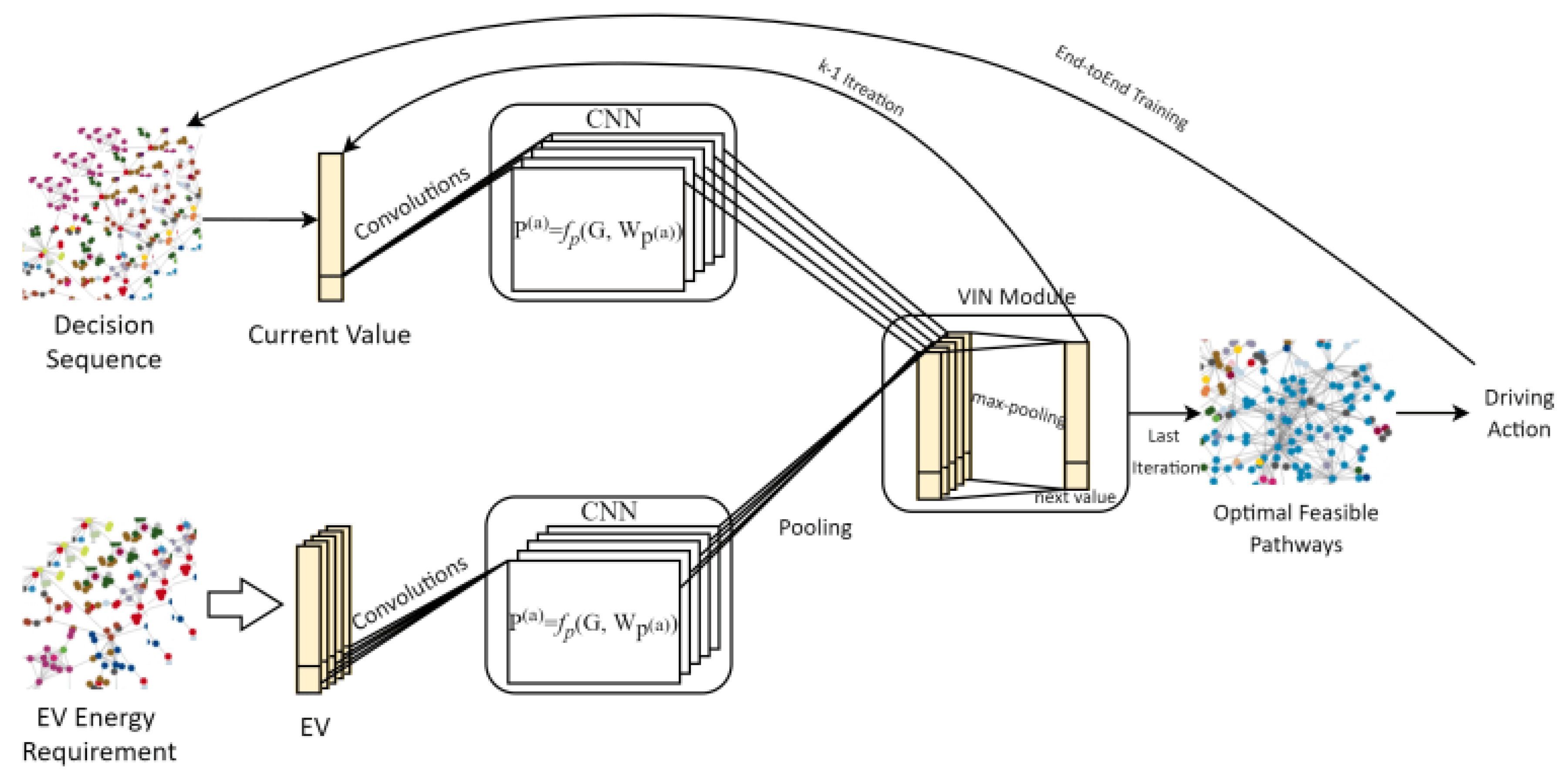
3.3. Value Iteration Network (VIN) Model

The main objective of designing the value-iteration network (VIN) is to find the optimal Q-values for the learning algorithm. Following the graph convolution and VIN, the traffic conditions of the agent could be mapped to routing decisions on the graph. To achieve this purpose, the VIN was approximated following the work of reference [36], where the VIN module was introduced as an NN layer that allows encoding differentiable planning computations. As proposed in [37], each iteration of the VIN module passes both value and reward functions through conventional neural network (CNN) max pooling layers. For optimal results, experienced replay inspired by [38] was integrated to allow a scalable learning model for the agent. To avoid getting the agent trapped in deciding optimal Q-values, a memory is utilized to store the output values of the previous learning iterations into a historical record stack. During the training process, training data from this stack are weight-sampled concerning its reward values. As Figure 3 shows, the input signal is an image representing geographical coordinates of the physical EV location, producing output that influences the overall travel policy following attention and observation. Then as shown in Figure 4, the quadrable ${\mathrm{e}}_{\mathrm{t}}=\langle \mathrm{s},\mathrm{a},\mathrm{r},\acute{\mathrm{s}},\acute{\mathrm{a}}\rangle$ is saved in historical stock $\mathrm{D}={\mathrm{e}}_1,{\mathrm{e}}_2, \dots , {\mathrm{e}}_n$, with $n$ as the number of the preserved states of the learning process. A CNN layer, fr, reforms the input grid map into one that contains pixels representing the reward values. The results from the MCM influence the value function described in Equations (1) and (8). Figure 5 provides illustration for the structure of the VI module in the training process. Particularly, at the i^th iteration, the loss function defined in Equation (11) is differentiated to get the gradient of the loss function. Finally, the output layer provides the optimal Q-values based on the discounting factor, save the quadrable in historical stack D, and then start the next iteration process. Values for the final policy values are produced once iterations are concluded.

3.4. Experimental Modeling of the EV’s Battery

A dynamic modeling of EV batteries was used for this simulation and was derived from the work of References [39,40]. Time factors for lithium batteries are presented in studies [41,42] and are incorporated into the battery model by [42] to better estimate SoC. The SoC, voltage, and power losses of the agent’s battery are modeled as follows:

$$V_{terminal}=V_{oc}\left(SOC,T\right)-i_{bat}\left(t\right)\times R_{int}\left(SOC,T\right)+i_{bat}\left(t\right)\times R_{transient}\left({\mathfrak{T}}_{sec},{\mathfrak{T}}_{min},{\mathfrak{T}}_{hour}\right)$$

(23)

where ${\mathfrak{T}}_{sec}$, ${\mathfrak{T}}_{min}$, and ${\mathfrak{T}}_{hour}$ represent time-constant variables of the dynamic behavior of the battery. It should be noted that number of driving cycles, temperature and battery’s discharge rate were assumed based on [42]. $V_{terminal}$ and $V_{oc}$ are both terminal and open circuit voltage levels for the battery’s circuit; $R_{int}$ and $R_{transient}$ are the battery’s internal and train set resistance; C_battery and I_battery represent the capacity and current of the battery, both modeled as a current source as follows [43]:

$$I_{SoC}=-I_{bat}\left(t\right)/C_{battery}$$

(24)

$$V_{SoC}=V_{terminal}/C_{battery}$$

(25)

Table 1 in Reference [42] shows the parameters utilized in our simulation, with the exception of the battery’s degradation level that was disregarded, as the battery’s life cyle is out of the scope of the study.

3.5. Impact of Regenerative Braking

To avoid having zero values in the diagonal elements of $T_M$ because of regenerative braking, a medial matrix is introduced in this work. Specifically, the medial matrix will allow only absolute values of the unit step of energy for the vehicle’s traveled path. Subsequently, the weights are rearranged as follows:

$$\left|W\right|=diag\left(\left|w_1\right|,\dots \dots ‥ ,\left|w_n\right|\right)$$

(26)

$$D=I-\propto {\left|W\right|}^{-1}$$

(27)

where $\propto$ represents the sign of a change of the energy requirement during regenerative braking and is strictly bounded in the interval 0 < $\propto$ < minimum $w_i$.

4. Results and Discussion

To verify the proposed energy minimization framework based on the SARSA algorithm, a real-time experiment was conducted in the Python environment to assess the capability of the proposed algorithm in achieving an optimal EV routing optimization. Furthermore, the energy required for the simulated trips based on Google Maps-suggested routes, and previously published results the authors had achieved following the DDQN algorithm [4] are benchmarks in this study. The overall goal of the experiment is to optimize the EV’s energy requirement by extending its driving range to navigate through what is typically considered a daily road trip that the average EV driver is expected to make. This experiment considers real-time metadata input that simulates a real-life driving condition to obtain realistic results. As an agent, the EV aims to maximize the reward of its decisions by reducing its energy requirement to reach a charging station that is assumed to be located six miles away from its driving starting point. This work successfully models the road segments’ dynamics between the two vertices through MCM. The EV was evaluated over 140 episodes, with each episode representing an entire set of steps, states, and reward signals obtained from the agent’s learning process. Termination criteria include either finishing the drive of a road’s segment or facing restrictions imposed on episodes. Such restrictions may include domain-specific restrictions (i.e., violation of permitted steps per episode), reaching an optimal energy-aware decision for driving that segment, or simply returning FALSE because of an unreachable step due to environment-specific limitations (e.g., flood, lakes, road closure, etc.). It is worth mentioning that this experiment considers two driving trips in two locations to measure the relative impact of the difference in the geophysical terrains on the learning algorithm. Both drives were simulated at 4.30 p.m., 11 October 2021. In addition, the importance of timesaving is neglected in his work, as we assumed that EV owners have limited energy in their batteries and that their main concerns are to reach their charging stations. The geophysical coordinates of the two selected drives are presented in

Table 3. Experimental information and results.

Simulated Trips	Starting Geocodes	Destination Geocodes	Energy by SARSA	Energy by Google’s Routes	Energy from Regenerative Braking	Simulation Time
FIU College of Engineering–Doral EV Charging Station	25.768506–80.366891	25.809732–80.331379	2.1305 Kwh at 21 min	2.3949 Kwh at 19 min	Negligible	3112 s
J. Paul Getty Museum -Ventura EV Charging Station	34.077823–118.475863	34.158980–118.49994	2.0501 Kwh at 25 min	2.1748 at 22 min	0.191 Kwh	2680 s

of this work. The first drive starts at the College of Engineering and Computing of the Florida International University (FIU), Miami, FL, whose destination is an EV charging station in Doral, FL, located nearly six miles away. The second drive, selected in a location that exhibits different geographic characteristics to add credibility to the testing of the proposed strategy, starts at the J. Paul Getty Museum, located in a hilltop area in Los Angeles, CA, USA. The destination of the second drive is set as a charging station in Ventura, CA, USA, which is also located six miles away from the starting location.

Table 4. Total number of episodes and steps per route.

Simulated Trips	No. of Episode	No. of Failed Step	Steps	Unreachable Positions
First Trip	140	20	5715	1711
Second Trip	143	18	7226	1501

highlights the total number of episodes and subsequent steps during the simulation of both drives. In addition, the experiment considered the stride length not to exceed 200 m, with 80 steps maximumly per each episode. As mentioned earlier, this experiment ignores timesaving, the battery’s level of degradation, and internal energy utilization of the EV (e.g., air conditioning). It is noted that different results may have been received depending on the condition of the dynamic environment, such as the time, location, distance, and driving routes.

The agent’s driving experience was simulated using Python with TensorFlow, Pandas, and NumPy libraries. A continuous update of the vehicle geocodes serves as input data for the learning algorithm, including data about the road such as traffic congestion, the highest and highest elevations on the roads, and speed limits, among others. Through Google’s API platform, real-time metadata information can be extracted from Google’s map services in real-time through APIs and software development kits (SDKs). It is worth mentioning that such a process was not easy to achieve, as we had to query the Direction API multiple times during the experiment to allow the proper representation of the drive considering the real-time traffic conditions per each road segment. Furthermore, the energy consumption of the agent was modeled for each state during the learning process to estimate the most optimal action per state. The results were then benchmarked with findings from a previous experiment achieved by the authors, considering the same driving experience but on different dates and algorithms. The results were also benchmarked when modeling the drive strictly following Google’s suggested routes. Figure 6 and Figure 7 present the energy requirements considering the proposed RL based on the SARSA algorithm, the DDQN algorithm, and Google’s original routes for both drives in Los Angeles, CA, USA, and Miami, FL, USA, respectively. As the results indicate, the EV reaches its planned destination with lower energy needs following the SARSA algorithm than the main route suggested by Google Maps, by 11.04% and 5.72%, respectively. Both drives took the same time to arrive at their destination, with a slight time difference of two minutes shorter in favor of Google Maps’ routes. As one may notice, although the exact vehicle was simulated for approximately the same length, there is a slight difference in the reported energy requirements. This could be attributed to the spatial and temporal differences in both driving experiences, which yielded slightly different energy requirements to reach each destination. Figure 8 shows a screenshot of the simulation results.

Table 3 presents the results of simulating the two trips. It is worth mentioning that the amount of regenerative braking is almost trivial, with only a small amount detected in the driving simulation in the Los Angeles trip. This is attributed to the relatively small distance driven by the agents and to the physical terrain of the LA drive, where a portion of the trip was driven downhill from the Santa Monica Mountains, where the J. Paul Getty Museum is located. Figure 9 and Figure 10 show the reward accumulation through the driving experience based on the SARSA algorithm considering 140 episodes. It should be noted that the reward is primarily influenced by the number of steps in the learning process, returning negative values whenever there is a failed episode. In addition, the EV’s returned reward is illustrated in Figure 9 and Figure 10 to provide insight into how much benefit the EV will receive from each action it takes at each state throughout the journey; it represents the accumulated sum at each time step t, following the discounted rate that was set earlier.

While the DDQN converged to slightly more optimal results than the SARSA algorithm, the learning process considering SARSA converged faster for both trips, as shown in Figure 11. This could be attributed to the fact that SARSA converges to the near-optimal policy as ε must be decayed so that the learning policy converges to a greedy policy, while the DDQN must achieve a full optimal policy. In addition, every state–action pair will be visited infinitely in SARSA. We had to limit the number of episodes in this experiment due to Google’s API restrictions, which limited and sometimes blocked our access to retrieve real-time data from the platform. As the training process proceeds, the agent’s random behavior decreases, indicating the learning algorithm’s robustness, as shown in Figure 12. The randomness that starts at the beginning of the drive is related to the fact that the agent starts the drive by taking random actions. Yet, such randomness decreases significantly as the SoC level improves due to the success of the learning algorithm in guiding the agent toward driving into energy-efficient options. As one may notice, as the agents continue the driving process, the reward trend indicates a positive direction with fewer negative values that are nothing but indicators of failed steps in the learning process. On a comparative scale, and as results presented in Figure 9, Figure 10 and Figure 11 show, the SARSA algorithm possesses unique characteristics that make it capable of solving difficult problems and this gives it an advantage over the popular Q-learning and DDQN algorithms. It has a faster convergence rate and accurate reward return when compared to Q-learning and can learn a near-optimal policy and remain more conservative, which means it seeks to avoid the risk of failure and hence opts for a longer and safer approach. If EMS and EV routing problems must be well probed in full detail with a lower risk of failure or errors along the way, the SARSA should be favored and put to more extensive use across the scientific community.

5. Conclusions

This work presents an energy consumption minimization framework based on the SARSA algorithm to train EVs to reach their final destinations with lower energy requirements. The dynamics of EVs on the road were modeled as successive partitioning that utilized the MCM to model the energy requirements for each partitioned segment. Two driving experiments of the same distance but at different geographic locations were simulated to verify the proposed framework. Both drives were set at a particular time and date with a limited state of charge, with the driving experience assumed to be a continuous state. As the agent incorporates real-time data from Google APIs, the transitional probabilities are updated continuously during the learning process. The results show the superiority of the SARSA algorithm in achieving optimal decisions for the agent to reach its destination with lower energy requirements than Google’s suggested routes at around the same traveling time. Compared with previously reported results by authors using DDQN [4] and Google’s originally suggested routes, the SARSA proved an effective learning strategy. Considering convergence performance and computation requirements, SARSA achieved better energy performance than Google’s routes but slightly less than the DDQN’s average driving time, which is only 15% over the driving period following Google’s routes. This shows that SARSA could exclude routes that may have resulted in a higher driving period even if they yield lower energy requirements. Due to its powerful computation capabilities, future work should incorporate the SARSA algorithm, as it has been proven to be an effective and reliable machine learning methodology. We recommend the implementation of the SARSA on topics such as smart grid reliability analysis studies [44,45], dynamic energy management systems incorporating EVs [46,47,48], and cybersecurity of energy grids such as charging stations [49]. However, a limitation to using the SARSA algorithm is that computational time may exceed that of other methods, as SARSA, a conservative RL method, may not execute the optimal solution within the shortest possible time. Due to its on-policy approach, the SARSA algorithm requires controllers to perform the action selection while following the policy for which the Q-values are found and updated. Another challenge to be investigated by the research community is the hardware implementation of ECU processors inside vehicles that incorporate AI algorithms such as the SARSA algorithm. Such implementation requires extensive integration efforts to achieve optimal real-time decisions for EV drivers. While previous microprocessors were presented in the literature by the ESRL of FIU to support smart charging decisions [50], ECU implementation that involves an AI-based algorithm system requires more extensive efforts to achieve optimal real-time decisions for EV drivers. References [51,52] highlight the real-time implementation of RL methods considering microprocessor capabilities. It is worth mentioning that better results of the SARSA algorithm may have been accomplished in this work if not for the continuous data interruptions from Google’s API platform, with the considerably limited computational capabilities of the simulating devices. Overall, the SARSA algorithm proved an effective RL methodology to train EVs to produce self-exploratory decisions that yield optimal driving decisions.

References

1. Pevec, D.; Babic, J.; Carvalho, A.; Ghiassi-Farrokhfal, Y.; Ketter, W.; Podobnik, V. Electric vehicle range anxiety: An obstacle for the personal transportation (r) evolution? In Proceedings of the 2019 4th International Conference on Smart and Sustainable Technologies (SpliTech), Split, Croatia, 18–21 June 2019; pp. 1–8. [Google Scholar]
2. Kim, S.; Rhee, W.; Choi, D.; Jang, Y.J.; Yoon, Y. Characterizing Driver Stress Using Physiological and Operational Data from Real-World Electric Vehicle Driving Experiment. Int. J. Automot. Technol. 2018, 19, 895–906. [Google Scholar] [CrossRef]
3. Van Hasselt, H.; Guez, A.; Silver, D. Deep Reinforcement Learning with Double Q-Learning. Proc. Conf. AAAI Artif. Intell. 2016, 30. [Google Scholar] [CrossRef]
4. Aljohani, T.M.; Ebrahim, A.; Mohammed, O. Real-Time metadata-driven routing optimization for electric vehicle energy consumption minimization using deep reinforcement learning and Markov chain model. Electr. Power Syst. Res. 2021, 192, 106962. [Google Scholar] [CrossRef]
5. Valogianni, K.; Ketter, W.; Collins, J.; Zhdanov, D. Effective management of electric vehicle storage using smart charging. In Proceedings of the Twenty-Eighth AAAI Conference on Artificial Intelligence, Québec City, QC, Canada, 27–31 July 2014. [Google Scholar]
6. Liu, T.; Zou, Y.; Liu, D.; Sun, F. Reinforcement Learning of Adaptive Energy Management With Transition Probability for a Hybrid Electric Tracked Vehicle. IEEE Trans. Ind. Electron. 2015, 62, 7837–7846. [Google Scholar] [CrossRef]
7. Qi, X.; Wu, G.; Boriboonsomsin, K.; Barth, M.; Gonder, J. Data-Driven Reinforcement Learning–Based Real-Time Energy Management System for Plug-In Hybrid Electric Vehicles. Transp. Res. Rec. J. Transp. Res. Board 2016, 2572, 1–8. [Google Scholar] [CrossRef] [Green Version]
8. Remani, T.; Jasmin, E.A.; Ahamed, T.P.I. Residential Load Scheduling With Renewable Generation in the Smart Grid: A Reinforcement Learning Approach. IEEE Syst. J. 2018, 13, 3283–3294. [Google Scholar] [CrossRef]
9. Rocchetta, R.; Bellani, L.; Compare, M.; Zio, E.; Patelli, E. A reinforcement learning framework for optimal operation and maintenance of power grids. Appl. Energy 2019, 241, 291–301. [Google Scholar] [CrossRef]
10. Ye, Y.; Qiu, D.; Sun, M.; Papadaskalopoulos, D.; Strbac, G. Deep Reinforcement Learning for Strategic Bidding in Electricity Markets. IEEE Trans. Smart Grid 2019, 11, 1343–1355. [Google Scholar] [CrossRef]
11. Perrusquía, A.; Yu, W.; Li, X. Multi-agent reinforcement learning for redundant robot control in task-space. Int. J. Mach. Learn. Cybern. 2021, 12, 231–241. [Google Scholar] [CrossRef]
12. Brunke, L.; Greeff, M.; Hall, A.W.; Yuan, Z.; Zhou, S.; Panerati, J.; Schoellig, A.P. Safe Learning in Robotics: From Learning-Based Control to Safe Reinforcement Learning. Annu. Rev. Control. Robot. Auton. Syst. 2022, 5, 411–444. [Google Scholar] [CrossRef]
13. Wang, Z.; He, H.; Wan, Z.; Sun, Y.L. Coordinated Topology Attacks in Smart Grid Using Deep Reinforcement Learning. IEEE Trans. Ind. Inform. 2020, 17, 1407–1415. [Google Scholar] [CrossRef]
14. An, D.; Yang, Q.; Liu, W.; Zhang, Y. Defending Against Data Integrity Attacks in Smart Grid: A Deep Reinforcement Learning-Based Approach. IEEE Access 2019, 7, 110835–110845. [Google Scholar] [CrossRef]
15. Oh, S.-Y.; Lee, J.-H.; Choi, D.-H. A new reinforcement learning vehicle control architecture for vision-based road following. IEEE Trans. Veh. Technol. 2000, 49, 997–1005. [Google Scholar]
16. Barrett, E.; Howley, E.; Duggan, J. Applying reinforcement learning towards automating resource allocation and application scalability in the cloud. Concurr. Comput. 2013, 25, 1656–1674. [Google Scholar] [CrossRef] [Green Version]
17. Liu, W.; Qin, G.; He, Y.; Jiang, F. Distributed Cooperative Reinforcement Learning-Based Traffic Signal Control That Integrates V2X Networks’ Dynamic Clustering. IEEE Trans. Veh. Technol. 2017, 66, 8667–8681. [Google Scholar] [CrossRef]
18. Huang, X.; Yuan, T.; Qiao, G.; Ren, Y. Deep Reinforcement Learning for Multimedia Traffic Control in Software Defined Networking. IEEE Netw. 2018, 32, 35–41. [Google Scholar] [CrossRef]
19. Ortiz, A.; Al-Shatri, H.; Li, X.; Weber, T.; Klein, A. Reinforcement learning for energy harvesting point-to-point communications. In Proceedings of the 2016 IEEE International Conference on Communications (ICC), Kuala Lumpur, Malaysia, 22–27 May 2016; pp. 1–6. [Google Scholar]
20. Luong, N.C.; Hoang, D.T.; Gong, S.; Niyato, D.; Wang, P.; Liang, Y.-C.; Kim, D.I. Applications of Deep Reinforcement Learning in Communications and Networking: A Survey. IEEE Commun. Surv. Tutorials 2019, 21, 3133–3174. [Google Scholar] [CrossRef] [Green Version]
21. Wang, S.; Bi, S.; Zhang, Y.J.A. Reinforcement Learning for Real-Time Pricing and Scheduling Control in EV Charging Stations. IEEE Trans. Ind. Inform. 2019, 17, 849–859. [Google Scholar] [CrossRef]
22. Aladdin, S.; El-Tantawy, S.; Fouda, M.M.; Eldien, A.S.T. MARLA-SG: Multi-Agent Reinforcement Learning Algorithm for Efficient Demand Response in Smart Grid. IEEE Access 2020, 8, 210626–210639. [Google Scholar] [CrossRef]
23. Wang, D.; Liu, B.; Jia, H.; Zhang, Z.; Chen, J.; Huang, D. Peer-to-peer electricity transaction decision of user-side smart energy system based on SARSA reinforcement learning method. CSEE J. Power Energy Syst. 2020, 8, 826–837. [Google Scholar]
24. Parque, V.; Kobayashi, M.; Higashi, M. Reinforced explorit on optimizing vehicle powertrains. In Proceedings of the International Conference on Neural Information Processing, Daegu, Korea, 3–7 November 2013; Springer: Berlin/Heidelberg, Germany, 2013; pp. 579–586. [Google Scholar]
25. Kouche-Biyouki, S.A.; Naseri-Javareshk, S.M.A.; Noori, A.; Javadi-Hassanehgheh, F. Power management strategy of hybrid vehicles using sarsa method. In Proceedings of the Electrical Engineering (ICEE), Mashhad, Iran, 8–10 May 2018; pp. 946–950. [Google Scholar]
26. Noel, L.; de Rubens, G.Z.; Sovacool, B.K.; Kester, J. Fear and loathing of electric vehicles: The reactionary rhetoric of range anxiety. Energy Res. Soc. Sci. 2019, 48, 96–107. [Google Scholar] [CrossRef]
27. Rummery, G.A.; Niranjan, M. On-Line Q-Learning Using Connectionist Systems; Department of Engineering, University of Cambridge: Cambridge, UK, 1994; Volume 37, p. 20. [Google Scholar]
28. Sutton, R.S.; Barto, A.G. Reinforcement Learning: An Introduction; MIT Press: Cambridge, MA, USA, 2018. [Google Scholar]
29. Cybenko, G. Approximation by superpositions of a sigmoidal function. Math. Control. Signals, Syst. 1989, 2, 303–314. [Google Scholar] [CrossRef]
30. Hinton, G.E.; Osindero, S.; Teh, Y.W. “A fast learning algorithm for deep belief nets” _(PDF). Neural Comput. 2006, 18, 1527–1554. [Google Scholar] [CrossRef] [PubMed]
31. Kumar, V. Reinforcement Learning: Temporal-Difference, SARSA, Q-Learning & Expected Sarsa on Python. Medium. Available online: https://towardsdatascience.com/reinforcement-learning-temporal-difference-sarsa-q-learning-expected-sarsa-on-python-9fecfda7467e (accessed on 12 May 2021).
32. Froyland, G. Extracting dynamical behavior via Markov models. In Nonlinear Dynamics and Statistics; Birkhauser: Boston, MA, USA, 2001; pp. 281–321. [Google Scholar]
33. Maia, R.; Silva, M.; Araujo, R.; Nunes, U. Electric vehicle simulator for energy consumption studies in electric mobility systems. In Proceedings of the IEEE Forum on Integrated and Sustainable Transportation Systems, Vienna, Austria, 29 June–1 July 2011; pp. 227–232. [Google Scholar]
34. Schlote Crisostomi, E.S.; Kirkland, R.; Shorten, R. Traffic modelling framework for electric vehicles. Int. J. Control 2012, 85, 880–897. [Google Scholar] [CrossRef]
35. Crisostomi, E.; Kirkland, S.; Shorten, R. Markov Chain based emissions models: A precursor for green control. In Green IT: Technologies and Applications; Kim, J.H., Lee, M.J., Eds.; Springer: Berlin/Heidelberg, Germany, 2011; pp. 381–400. [Google Scholar]
36. Apostolaki-Iosifidou, E.; Codani, P.; Kempton, W. Measurement of power loss during electric vehicle charging and discharging. Energy 2017, 127, 730–742. [Google Scholar] [CrossRef]
37. Tamar, A.; Wu, Y.; Thomas, G.S.; Levine; Abbeel, P. Value iteration networks. Adv. Neural Inf. Process. Syst. 2016, 9, 2146–2154. [Google Scholar]
38. Gold, S. A PSPICE macromodel for lithium-ion batteries. In Proceedings of the 12th Annual Battery Conference on Applications and Advances, Long Beach, CA, USA, 14–17 January 1997; pp. 215–222. [Google Scholar]
39. Kroeze, R.C.; Krein, P.T. Electrical battery model for use in dynamic electric vehicle simulations. In Proceedings of the 2008 IEEE Power Electronics Specialists Conference, Rhodes, Greece, 15–19 June 2008; pp. 1336–1342. [Google Scholar]
40. Chen, M.; Rincon-Mora, G.A. Accurate electrical battery model capable of predicting runtime and I-V performance. IEEE Trans. Energy Convers. 2006, 21, 504–511. [Google Scholar] [CrossRef]
41. Schweighofer, B.; Raab, K.M.; Brasseur, G. Modeling of high-power automotive batteries by the use of an automated test system. IEEE Trans. Instrum. Meas. 2003, 52, 1087–1091. [Google Scholar] [CrossRef]
42. Gao, L.; Liu, S.; Dougal, R. Dynamic lithium-ion battery model for system simulation. IEEE Trans. Components Packag. Technol. 2002, 25, 495–505. [Google Scholar]
43. Sun, C.; Moura, S.J.; Hu, X.; Hedrick, J.K.; Sun, F. Dynamic Traffic Feedback Data Enabled Energy Management in Plug-in Hybrid Electric Vehicles. IEEE Trans. Control Syst. Technol. 2015, 23, 1075–1086. [Google Scholar]
44. Aljohani, T.M. Distribution System Reliability Analysis for Smart Grid Applications; University of Southern California: Los Angeles, CA, USA, 2014. [Google Scholar]
45. Aljohani, T.M.; Beshir, M.J. Matlab code to assess the reliability of the smart power distribution system using monte carlo simulation. J. Power Energy Eng. 2017, 5, 30–44. [Google Scholar] [CrossRef] [Green Version]
46. Alqahtani, M.; Hu, M. Dynamic energy scheduling and routing of multiple electric vehicles using deep reinforcement learning. Energy 2022, 244, 122626. [Google Scholar] [CrossRef]
47. Aljohani, T.M.; Ebrahim, A.F.; Mohammed, O.A. Dynamic real-time pricing mechanism for electric vehicles charging considering optimal microgrids energy management system. IEEE Trans. Ind. Appl. 2021, 57, 5372–5381. [Google Scholar] [CrossRef]
48. Yang, T.; Zhao, L.; Li, W.; Zomaya, A.Y. Reinforcement learning in sustainable energy and electric systems: A survey. Annu. Rev. Control. 2020, 49, 145–163. [Google Scholar] [CrossRef]
49. Aljohani, T.M. Cyberattacks on Energy Infrastructures: Modern War Weapons. arXiv 2022, arXiv:2208.14225. [Google Scholar]
50. Hariri, A.; El Hariri, M.; Youssef, T.; Mohammed, O. Systems and Methods for Electric Vehicle Charging Decision Support System. U.S. Patent 10,507,738, 17 December 2019. [Google Scholar]
51. Dini, P.; Saponara, S. Processor-in-the-Loop Validation of a Gradient Descent-Based Model Predictive Control for Assisted Driving and Obstacles Avoidance Applications. IEEE Access 2022, 10, 67958–67975. [Google Scholar] [CrossRef]
52. Ramstedt, S.; Pal, C. Real-time reinforcement learning. In Proceedings of the Advances in Neural Information Processing Systems, Vancouver, BC, Canada, 8–14 December 2019; p. 32. [Google Scholar]
Figure 1. Learning process in the RL (environment) algorithm.
Vehicles 04 00062 g001
Figure 2. Illustration of graph representation considering MCM.
Vehicles 04 00062 g002
Figure 3. Illustration of the VIN structure utilized in the learning process.
Vehicles 04 00062 g003
Figure 4. Illustration of the data extraction mechanism in this work.
Vehicles 04 00062 g004
Figure 5. Illustration of the value function feedback iterations in the learning process.
Vehicles 04 00062 g005
Figure 6. Benchmarking of the energy requirements of the first route for SARSA vs. DDQN and Google Maps.
Vehicles 04 00062 g006
Figure 7. Benchmarking of the energy requirement for the second route for SARSA vs. DDQN and Google Maps.
Vehicles 04 00062 g007
Figure 8. Part of the simulation process for the second drive in Los Angeles, CA, USA.
Vehicles 04 00062 g008
Figure 9. Accumulated reward returns per the number of steps in the first trip.
Vehicles 04 00062 g009
Figure 10. Accumulated reward returns per the number of steps in the second trip.
Vehicles 04 00062 g010
Figure 11. Convergence performance of the two RL-proposed algorithms.
Vehicles 04 00062 g011
Figure 12. The level of SoC vs. probability of taking random actions for the agent during the drives.
Vehicles 04 00062 g012