Nature-Inspired Optimal Route Network Design for Shared Autonomous Vehicles

Abstract

Emerging forms of shared mobility call for new vehicle routing models that take into account vehicle sharing, ride sharing and autonomous vehicle fleets. This study deals with the design of an optimal route network for autonomous vehicles, considering both vehicle sharing and ride sharing. The problem is modeled as a one-to-many-to-one vehicle routing problem with vehicle capacity and range constraints. An ant colony optimization algorithm is applied to the problem in order to construct a set of routes that satisfies user requests under operational constraints. Results show that the algorithm is able to produce solutions in relatively short computational times, while exploiting the possibility of ride sharing to reduce operating costs. Results also underline the potential of exploiting shared autonomous vehicles in the context of a taxi service for booking trips through electronic reservation systems.

1. Introduction

In recent years, flexible and environmentally friendly mobility options have emerged in cities in an effort to reduce private vehicle usage. Spurred by the rise of the collective economy, vehicle sharing has been at the core of these efforts, aiming at lower travel costs per user and reduced pollutants [1]. Similar benefits result from ride sharing, where customers with different routes are served by the same vehicle for a part of their route [2]. Recently, developments in the field of autonomous vehicles have shifted research interests towards shared autonomous vehicles (SAVs) that can simultaneously transport passengers with different origins and destinations by exploiting common route segments and can be used as taxis [3]. These vehicles exploit artificial intelligence and sensor systems, enabling them to perceive the surrounding environment and react accordingly. The wide deployment of these vehicles is expected to change the reality of urban transport. Indeed, studies have shown that SAVs could replace anywhere between 3 and 11 private cars [3,4]. At the same time, the exploitation of alternative energy sources by exploiting electric and hybrid autonomous vehicle fleets can lead to further reductions in pollutants in urban centers [5].

The determination of efficient routes is crucial for fully exploiting the capabilities offered by SAVs in the context of flexible mobility. The associated vehicle routing problem (VRP), which refers to the determination of optimal routes originating from a central depot to a set of customers under capacity constraints, has been studied for several decades under various objectives and operational settings [6]. However, for the case of shared autonomous electric vehicles, route design must simultaneously consider range constraints and the possibility of ride sharing [7]. The latter requires additional methodological and algorithmic treatment as typical VRP models consider demand to/from a central depot. Despite the interest shown for shared autonomous vehicles, the planning of shared routes and electrification has not received adequate attention in the literature. In light of the above, the paper proposes an optimal route network design model for autonomous electric vehicles, considering both vehicle sharing and ride sharing.

Vehicle routing problems with pick-ups and deliveries can include delivery first, pick-up second, mixed pick-ups and deliveries or simultaneous pick-ups and deliveries [8]. In its general form, the problem of providing demand-responsive transportation services under vehicle and ride sharing is a “VRP with simultaneous pick-ups and deliveries”, which shares some characteristics with the dial-a-ride problem (DARP). The goal in the latter is to satisfy a set of traveler requests with specific origins and destinations with minimum costs. In general, DARP models also focus on mitigating the consequences of traffic congestion, such as increased user travel times [9,10], reduced service reliability [11,12] and increased gas emissions [13,14]. Typically, DARPs are classified as static or dynamic, based on the nature of the travel demand. In static variants, demand is assumed to be known in advance [15], while in dynamic ones, new service requests may be generated during the solution process [16]. In any case, these problems, as extensions of the VRP (which is a known NP-hard problem) are computationally expensive, while they often need to be solved either fast or in real time [15,16]. NP-hard problems cannot be solved exactly for large instances as their complexity rises exponentially with the problem size [8]. For this reason, the development of appropriate heuristic and metaheuristic algorithms has been extensively studied [17,18,19,20].

In recent years, research attention has shifted to DARP formulations considering shared vehicles and routes. In this line of research, a branch of studies has focused on relevant variations considering ride sharing between drivers and passengers [2,21]. Similarly, vehicle sharing, which typically refers to short-term car rental through online reservation, has been extensively studied and has been found to reduce the number of trips and vehicles [22,23]. In a similar context, De Almeida Correia and van Arem [24] investigated the impact of privately owned SAVs in terms of traffic congestion and parking demand, also noting reduced vehicle trips and generalized travel costs. Recently, Bongiovanni et al. [6] formulated the DARP for electric autonomous vehicles as a mixed-integer linear programming model able to handle small-scale instances.

Despite the growing interest for autonomous vehicles, SAV network design in the context of flexible mobility services has not received the appropriate attention [25,26]. Optimal solutions to the SAV routing problem under ride sharing could lead to reduced travel and wait times and notably decrease transportation cost for users and operators. Several studies have used simulation for planning SAV routes, exploring the potential benefits at a macroscopic level [3,23] or microscopic level [27]. Another branch of studies has proposed models for the real-time routing of SAVs. Alonso-Mora et al. [25] proposed a mathematical model for planning autonomous vehicle sharing in real time, employing a hybrid heuristic methodology for its solution. Ge et al. [28] presented a scheduling and routing model for SAV routing under congestion, presenting a convex formulation. In a similar context, Venkatraman and Levin [29] proposed a tabu search heuristic for congestion-aware SAV routing. Similarly, Aziz et al. [26] also employed a tabu search algorithm for route planning in the context of on-demand shared mobility services. However, attention must be given to ride-sharing patterns in these studies, as passenger discomfort considerations arise due to detours [30,31]. Li et al. [32] presented mixed-integer linear programming models for people–freight taxi sharing, addressing both static and dynamic scenarios, with a maximum detour length considered. Santos and Xavier [31] presented a greedy randomized adaptive search to solve the dynamic ride-sharing problem for taxis, taking into account the maximum accepted delay of passengers. The authors handled the dynamic problem by decomposing it into static problems.

Nevertheless, we assume the vehicle routing problem for SAVs to be static, therefore routes must be scheduled a priori to satisfy known customer requests. Moreover, the static problem can be used for handling dynamic cases, as empirical results demonstrating similar behavior to the dynamic case [32] while decomposition approaches of a dynamic problem into multiple static instances can be successfully used as well [31,33]. Therefore, a static framework for implementing a taxi ride-sharing service can be very useful. This paper investigates vehicle routing for SAVs in the context of regular customers who travel according to a predefined schedule, e.g., commuting for work. For instance, such an approach could apply in the case of micro-transit services, where passengers pre-book their trips through online reservation systems. The objective is to find the minimum distance traveled by all vehicles until all customers are served under capacity and maximum range constraints. Furthermore, ride sharing is considered in a flexible manner, as partial, internal and complete sharing can occur [30]. Insertion operators for the algorithmic treatment of ride sharing are costly and often ineffective, resulting in expensive computational methods [30,31,32,33,34]. In this context, we propose a computationally efficient targeted insertion method for ride sharing that organically considers passengers’ inconvenience. The problem is then solved by an appropriately modified ant colony optimization algorithm for handling the operational conditions of electric fleets and ride sharing, which, to our knowledge, is applied to the problem at hand for the first time. The algorithm is applied to an urban network in Athens, Greece, where 30 service points are considered around the city. The remainder of the paper is organized as follows. Next, the mathematical formulation is provided and the solution algorithm is presented in Section 2. Subsequently, computational results are presented and analyzed in Section 3. The paper concludes with findings and research gaps in Section 4.

2. Materials and Methods

The problem is formulated as a DARP, considering both vehicle sharing and ride sharing. Demand is known at the beginning of the planning horizon, while the set of pick-up and drop-off locations is predetermined. Customers can make travel requests online, using either a website or a mobile application by selecting an origin and destination node from a set of pick-up and drop-off points. Similar to current practices in the online reservation of “shared van” services, it is assumed that customer requests may be accepted until a specific point in time before the beginning of service provision. This study also considers the use of battery electric vehicles and the associated range constraints applying. Vehicles start from and return to a main depot, where charging is possible, until all customers are served (one-to-many-to-one VRP).

2.1. Mathematical Model

The service network can be represented as a graph G = (N,A), where N = {0,1,…,n} is the set of nodes and node 0 represents the depot. A maximum vehicle capacity Q is assumed. Each vehicle can traverse an arc i-j, either if nodes i,j represent the origin and destination node for a customer request, respectively, or if node i is the customer’s drop-off destination and node j is the origin node of the next group of customers to be picked up. The optimization goal is to minimize the system-wide operating cost, which is reflected by the total distance traveled by all vehicles.

Let:

Indices

i,j: nodes;

m: vehicle.

Sets

M: set of vehicles;

N: set of nodes.

Parameters

Q: maximum capacity of each vehicle;

c_ij: distance between nodes i,j.

Variables

$Q_i^m$: load of vehicle m departing from node i;

$q_i^m$: number of travelers on node i that will be served by vehicle m;

$x_{ij}^m$: binary variable that indicates if arc i j is served by vehicle m;

L: maximum distance that can be traversed by a vehicle.

The problem is then formulated as follows:

$$\min Z={\displaystyle \sum _{m\in M}{\displaystyle \sum _{i\in N}{\displaystyle \sum _{j\in N}{c}_{ij}\cdot }{x}_{ij}^m}}$$

(1)

subject to:

$$x_{ij}^m=\left\{\begin{array}{l}1, \mathrm{if} \mathrm{vehicle} m \mathrm{traverses} \mathrm{arc} ij\\ 0, \hspace{1em}\hspace{1em}\hspace{1em}\mathrm{otherwise}\end{array}\right\}$$

(2)

$${\displaystyle \sum _{j\in N}{x}_{ij}^m=1}\hspace{1em}\hspace{1em}\hspace{1em}\hspace{1em}\forall i\in N,m\in M$$

(3)

$${\displaystyle \sum _{j\in N}{x}_{ij}^m=}{\displaystyle \sum _{i\in N}{x}_{ij}^m}\hspace{1em}\hspace{1em}\hspace{1em}\hspace{1em}\forall i\in N,j\in N,m\in M$$

(4)

$$Q_j^m\ge (Q_i^m+q_j^m)\cdot x_{ij}^m\hspace{1em}\hspace{1em}\hspace{1em}\hspace{1em}\forall i\in N,j\in N,m\in M$$

(5)

$$\max \left\{0,q_i^m\right\}\le Q_i^m\le \min \left\{Q,Q_i^m+q_i^m\right\}\hspace{1em}\hspace{1em}\hspace{1em}\hspace{1em}\forall i\in N,m\in M$$

(6)

$${\displaystyle \sum _{i\in N}{\displaystyle \sum _{j\in N}{c}_{ij}\cdot }{x}_{ij}^m}\le L\hspace{1em}\hspace{1em}\hspace{1em}\hspace{1em}\forall m\in M$$

(7)

$${\displaystyle \sum _{j\in N}{x}_{0j}^m}=1\hspace{1em}\hspace{1em}\hspace{1em}\hspace{1em}\forall m\in M$$

(8)

$${\displaystyle \sum _{i\in N}{x}_{i0}^m}=1\hspace{1em}\hspace{1em}\hspace{1em}\hspace{1em}\forall m\in M$$

(9)

$$x_{ij}^m\in S\hspace{1em}\hspace{1em}\hspace{1em}\hspace{1em}\forall i\in N,j\in N,m\in M$$

(10)

$$S=\left\{x_{ij}^m:{\displaystyle \sum _{i\in B}{\displaystyle \sum _{j\in B}{x}_{ij}^m\le \left|B\right|-1,B\subseteq N,\left|B\right|\ge 2}}\right\}$$

(11)

The objective function Z (Equation (1)) minimizes the total distance traveled. Equation (2) defines the decision variables. Constraints (3) and (4) ensure that each request is served exactly once and that the origin and destination nodes are visited by the same vehicle. Capacity constraints are imposed by Equations (5) and (6) [35]. Equation (7) ensures that vehicle maximum range will not be exceeded. Constraints (8) and (9) ensure that each vehicle starts and ends its route at the depot. Constraints (10) and (11) ensure sub-tour elimination. The problem formulated in Equations (1)–(11) is a non-linear mixed-integer model.

2.2. Solution Algorithm

In terms of complexity, the VRP is NP-hard, as there is no polynomial algorithm able to find the optimal solution [36]. Therefore, it can be exactly solved only for small instances [37,38]. Consequently, the use of heuristic and metaheuristic algorithms has been the most popular approach for routing problems [39,40]. A popular metaheuristic algorithm widely applied to VRP variants is ant colony optimization [41,42]. This algorithm employs artificial ants to find solutions to combinatorial optimization problems, mimicking the mechanism for locating food observed in real-world ant colonies. The algorithm emulates the behavior of ants and includes enhanced abilities such as collective memory and knowledge. The self-learning process and probabilistic decision making based on the ants’ collective knowledge make this algorithm very attractive for solving network design problems. In VRPs, pheromone evaporation and pheromone reinforcement processes are used to guide the search [43,44]. The pheromone evaporation is employed for uniformly decreasing the pheromone values on all arcs and aims at reducing the probability of repeatedly selecting a customer. The pheromone reinforcement increases the probability of selecting the arcs used by many ants and belonging to short tours [44]. Ant-based algorithms have been successfully applied for solving combinatorial optimization problems such as the traveling salesman problem as well as the VRP and its variants [36,43,44]. For this reason, an ant colony optimization approach is applied, with a tailored sub-routine incorporated to insert requests so that partial ride sharing can be exploited to allow ride sharing between passengers and to ensure compliance with the maximum range limitation.

2.2.1. Solution Representation

An integer representation scheme is used. Each node in the network is assigned a number from 0 to 30, with a string representing a route. Further, node 0 represents the depot from where the vehicles depart and must return to before the end of the shift, while there is no demand from and to this point. For instance, assuming requests 1–19, 2–6, 3–16, 4–16, 5–7, one solution could be expressed as follows:

[0,3,4,16,0]: Route of vehicle A

[0,1,19,2,6,0]: Route of vehicle B

[0,5,7,0]: Route of vehicle C

2.2.2. Initialization

Initially, a solution is constructed using the nearest neighbor heuristic in order to enhance the pheromone of the shortest paths [44]. An initial amount of pheromone is deposited on each arc, equal to the inverse of its length. The process repeatedly adds nodes to a path so that the vehicle starting from the depot visits the nearest node, continues until all nodes have been visited and returns to the depot.

2.2.3. Route Construction

In the ant colony optimization, an ant represents a vehicle and its route is gradually constructed choosing nodes until all passengers are served. Route construction steps are presented below [36,44].

Step 1: Node selection

Every ant starts from the route-initiating node. The ant chooses the next node to be visited from a list of candidate locations, which can be reached from its position without violating range constraints. The remaining vehicle capacity is subsequently updated. In this case, before adding a node to a route and considering a customer request as satisfied, it must first be checked whether the vehicle can travel until the pick-up node, continue to the customer’s destination and then return to the depot without exceeding the maximum range constraint. If this condition is met, both the pick-up node and the node representing the customer’s destination are added to the route. In order to select the next node to be inserted, the algorithm uses the following probability equation [36]:

$$\mathrm{Pij} =\frac{\left(t_{ij}\right)\left(n_{ij}^{\beta }\right)}{{{\displaystyle \sum }}_{u\notin M_k}(t_{iu})\left(n_{iu}^{\beta }\right)}$$

(12)

where t_iu is the total amount of pheromone on the path from node i to all the candidate nodes u. Variable n_ij is defined as the inverse of the distance between two locations, while positive parameter β determines the importance attributed to distance over the amount of pheromone. Nodes that have already been visited by an ant are stored in memory and excluded from the selection. Equation (12) is used when a random variable q exceeds the value of parameter q₀. The latter determines the importance of exploiting already existing information compared with the exploration of new solutions. Otherwise, the ant randomly chooses a customer. Once a complete route is constructed by the first ant through this process, the second ant constructs its own route.

Step 2: Route Construction for each Vehicle

The above process continues until a predetermined number of ants m construct their own feasible routes. The vehicle returns to the depot when capacity and range constraints are exhausted.

The process is completed when all customers are served or when there are no other available vehicles.

2.2.4. Updating Pheromone Trail Intensity

In order to improve subsequent selections of ants, traces of pheromone must be updated to reflect the ants’ performances and the quality of the solutions that have been already found. This update includes both local path updates once individual solutions are created and global updates based on the best set of routes found.

Local Update

Local update is performed by reducing the amount of pheromone for all nodes that have been visited by a vehicle, aiming to simulate natural pheromone evaporation, ensuring that no link will accumulate all the pheromone quantity. This is performed with the following pheromone local update equation [36]:

$${\mathrm{t}}_{\mathrm{ij}}=\left(1-\mathrm{a}\right){\mathrm{t}}_{\mathrm{ij}}+{ \mathrm{a}\ast \mathrm{t}}_0$$

(13)

where a is a parameter that controls the speed of evaporation and t₀ is the initial value of the pheromone intensity that has been set to the arcs of graph G. In this study, the amount for each arc is initialized as the inverse of the distance between its nodes.

Global Update

When all ants have created a complete solution, i.e., a route set, the global update of pheromone-trail intensities is conducted. In other words, pheromone values in all arcs that are included in the shortest route found by an ant (vehicle) are updated, according to the following equation [36]:

$${\mathrm{t}}_{\mathrm{ij}}=(1-\mathrm{a})\ast { \mathrm{t}}_{\mathrm{ij}}+\mathrm{a}/\mathrm{L}$$

(14)

where L is the length of the shortest route.

This way, the probability that arcs included in the best solutions will be selected per Equation (12) in future routes is increased. This process is repeated for a predetermined number of iterations and the best solution of all iterations is the final result of the model.

2.2.5. Iteration Termination

When a complete set of routes that minimizes the objective function is generated, a new experiment starts. The only parameter that is not restored to the initial value is the amount of pheromone for each origin–destination pair, as knowledge of the previous values is exploited. The process terminates when all experiments for a number of iterations that has been set by the user are operated.

2.2.6. Ride Sharing Treatment Process

Once the iterative procedure is completed, in order to reduce the total distance traveled by all SAVs, the algorithm checks whether there are routes that exclusively serve a single traveler request. If such routes exist, the next step is to check whether the corresponding traveler requests can be served from an existing route by examining vehicle loads on the corresponding route segments. If these origin–destination pairs can be served from other routes without violating range and capacity constraints, redundant routes are deleted and the corresponding passengers are assigned to the vehicles serving these routes.

3. Results

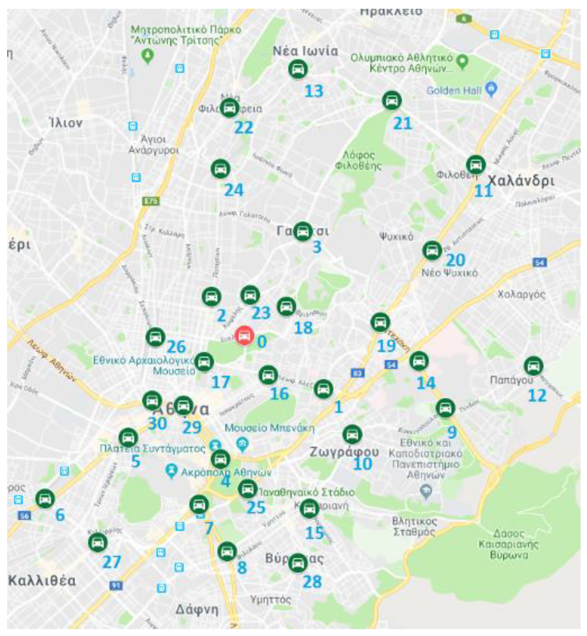
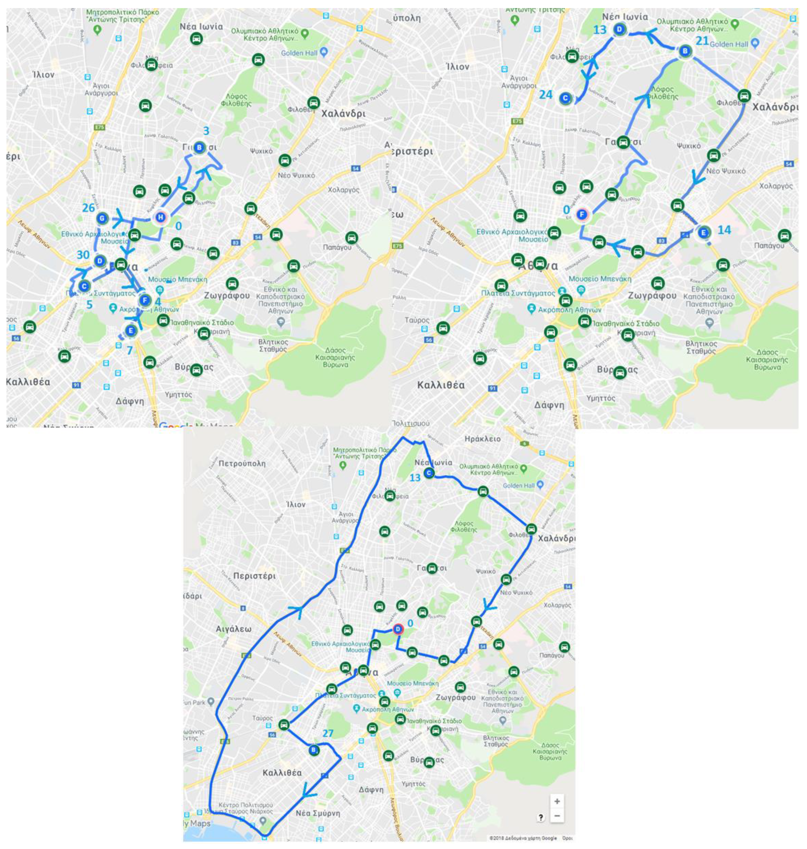
The algorithm is implemented in Python 2.7 and run on a computer with a 3.0 GHz processor and a 5.0 GB RAM. A set of 30 points in the central area of Athens is chosen as a testbed with corresponding points shown in Figure 1, where the stops and the starting node (depot) are shown with green and red colors, respectively. Furthermore, the travel time matrix is derived using Google Maps, using the shortest distance and avoiding freeways wherever possible.

Passenger demand was randomly generated while ensuring that there was a request originating from each network node, with the destination randomly chosen each time. The number of passengers per request was randomly assigned a value between one and four. A maximum distance of 29 km (18 m) [45] was considered for each route based on range and time duration constraints [3], while the available fleet size was set to 30 vehicles. We used 30 vehicles because we considered 30 requests so that, even if no ride sharing was used, the demand could still be served in the worst-case scenario. A homogeneous autonomous vehicle fleet was assumed, while vehicle capacity was set to four passengers. Time windows within which customer demand must be accommodated were not considered, as the limited vehicle range and the restriction on route duration did not allow for long routes anyway. Furthermore, passengers were assumed to be commuters traveling within specific periods of the day, while all autonomous vehicles departed at the same time from the same starting node. Since the start time was predefined, the maximum distance constraint considered also indirectly handled passengers’ timing constraints. Similar to Fagnant and Kockelman [3], we assumed that fixed speeds could be pre-set by time of day, thus distance could be used interchangeably with travel time in our case, as the service was intended for a specific period (morning commute). The generated passenger demand matrix is presented in

Table 1. Customer demand.

Origin Node	Destination Node	Number of Customers
1	14	2
2	12	4
3	5	1
4	26	4
5	1	4
6	16	1
7	27	2
8	3	2
9	17	1
10	19	2
11	2	4
12	22	1
13	14	3
14	22	1
15	5	3
16	8	4
17	4	1
18	16	1
19	28	1
20	18	3
21	24	1
22	12	1
23	4	2
24	9	4
25	21	2
26	22	2
27	13	3
28	3	1
29	9	3
30	7	1

, where origin and destination nodes are shown along with the number of customers per request.

3.1. Algorithm Calibration

The process of algorithm calibration relates to the determination of the best combination for the parameters used as input in the optimization process. The following parameters were examined:

Pheromone evaporation parameter a: This variable is used for updating pheromone trail intensity for an arc. Its purpose is to simulate the natural process of evaporation. According to the literature, its values can range between 0 and 1 (0 ≤ a ≤ 1) [44]. Three values of parameter a are examined, namely 0.1, 0.5 and 0.8, to simulate a slow, medium and fast evaporation rate [36,44,46]

Parameter β: This dictates the importance of distance in comparison with pheromone quantity. As mentioned before, probability P_ij, which significantly affects node selection, is calculated by Equation (12). In this case, the values examined are 0.5,1 and 2 [44].

The comparison was based on the best value of the objective function; 30,000 iterations for each combination were performed. Execution times ranged between 5 and 6 min for 30,000 experiments.

As can be observed from

Table 2. Objective function values for different a and β combinations.

a	β	L (m)
0.1	0.5	288,000
	1	286,300
	2	286,300
0.5	0.5	285,300
	1	286,500
	2	285,300
0.8	0.5	286,800
	1	285,300
	2	286,500

, the best value of the objective function, namely L = 285,300 m, appears in the following cases:

• a = 0.5 and β=0.5;
• a = 0.5 and β=2;
• a = 0.8 and β=1.

Out of these three combinations, the first one, which puts more emphasis on pheromone quantity compared with distance, is selected.

Table 3. Algorithm results.

Vehicle	Route
1	[0,18,16,17,4,25,21,0]
2	[0,23,4,7,27,6,16,1,14,20,18,0]
3	[0,2,12,14,22,0]
4	[0,5,1,10,19,11,2,0]
5	[0,16,8,28,3,0]
6	[0,22,12,9,17,0]
7	[0,29,9,19,28,15,5,0]
8	[0,26,22,24,9,0]
9	[0,3,5,30,7,4,26,0]
10	[0,21,24,13,14,0]
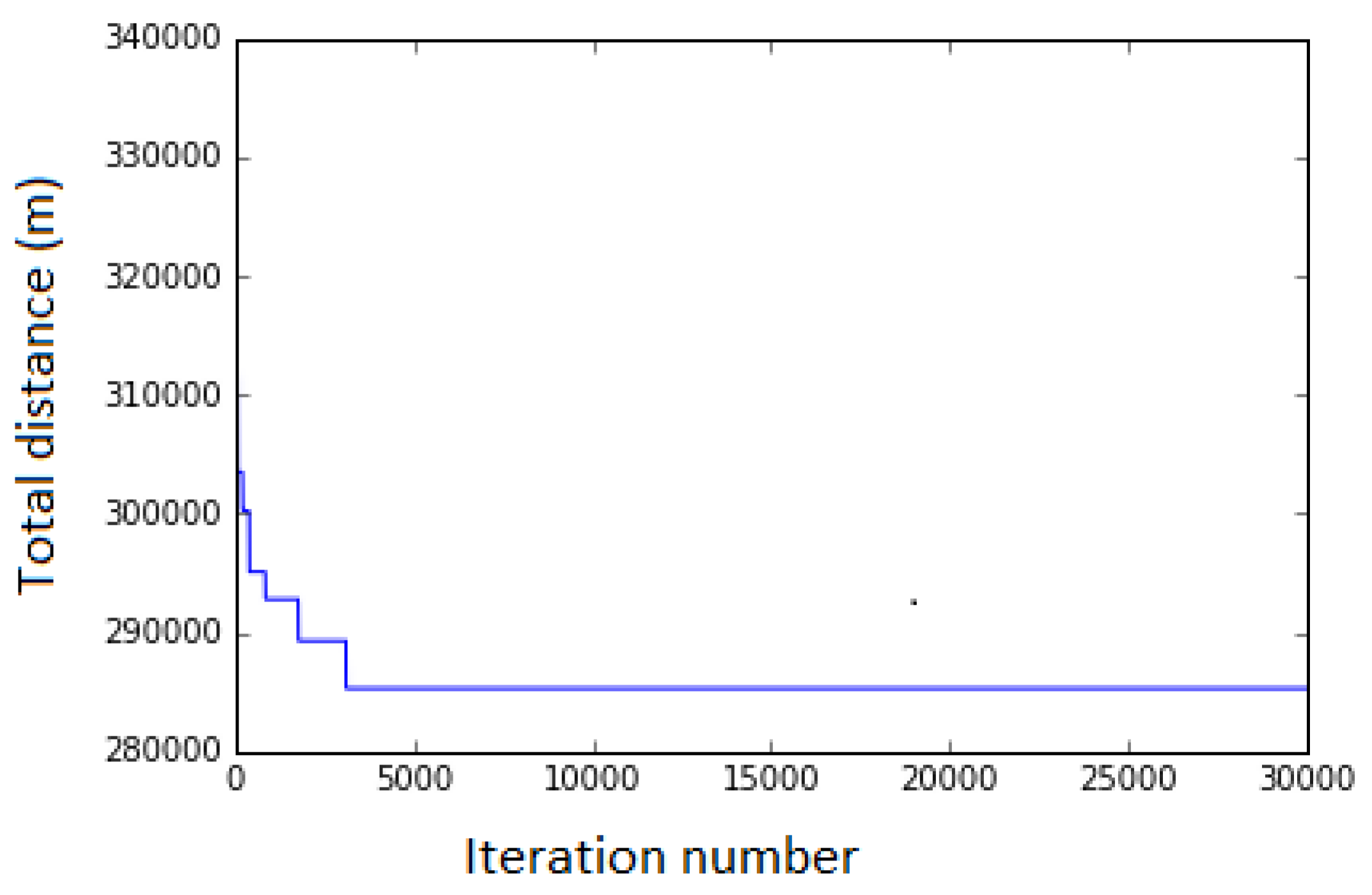
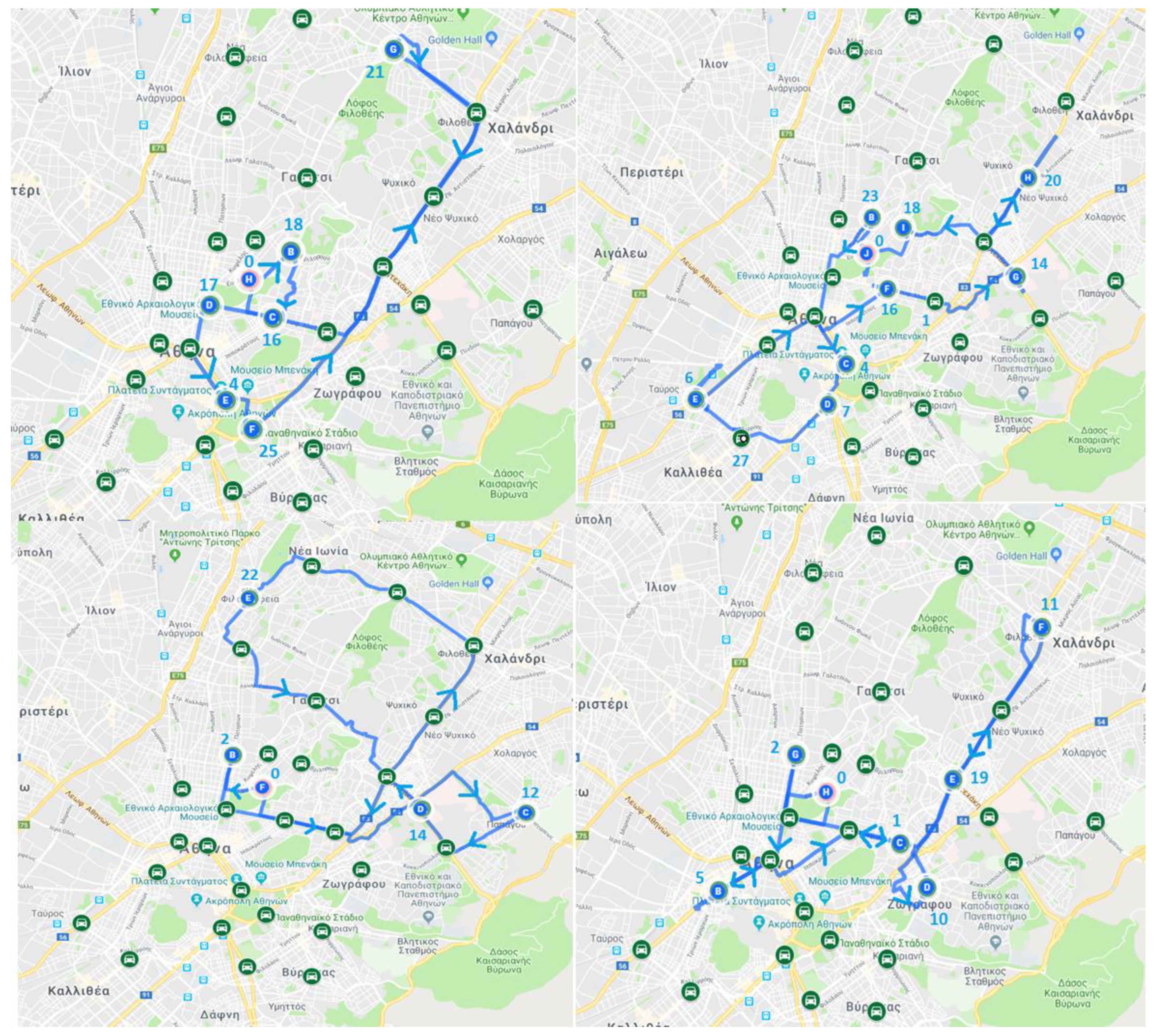
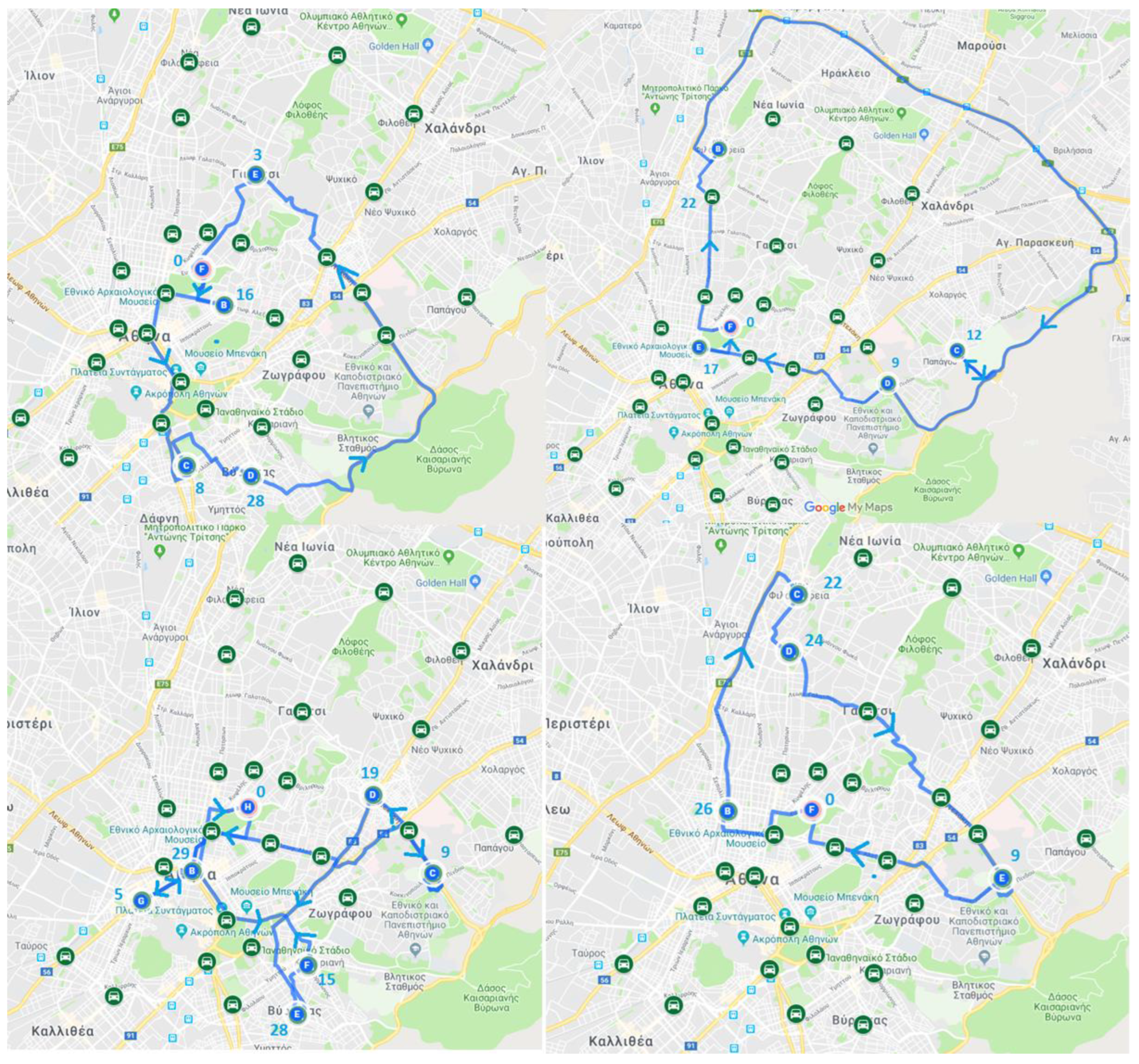
11	[0,27,13,0]

shows the resulting vehicle routes corresponding to the best solution at a cost of 285.30 km. Time durations for the longest and the shortest routes are 35.96 and 26.76 min, respectively, which are considered acceptable in the context of a shared ride service. Taking a closer look at the results, ride sharing is used twice and, specifically, in the case of vehicles 3 and 5 for requests 12–22 and 8–3, respectively.

It should be noted that for any value of fleet size above 11 vehicles the solution is the same, while for any value under 11 the problem is infeasible due to capacity and range constraints. The evolution of the objective function values during the optimization process is presented in Figure 2. As seen, a best value is found relatively fast (before 5000 iterations).

Vehicle routes are shown in Figure 3, Figure 4 and Figure 5.

3.2. Sensitivity Analysis

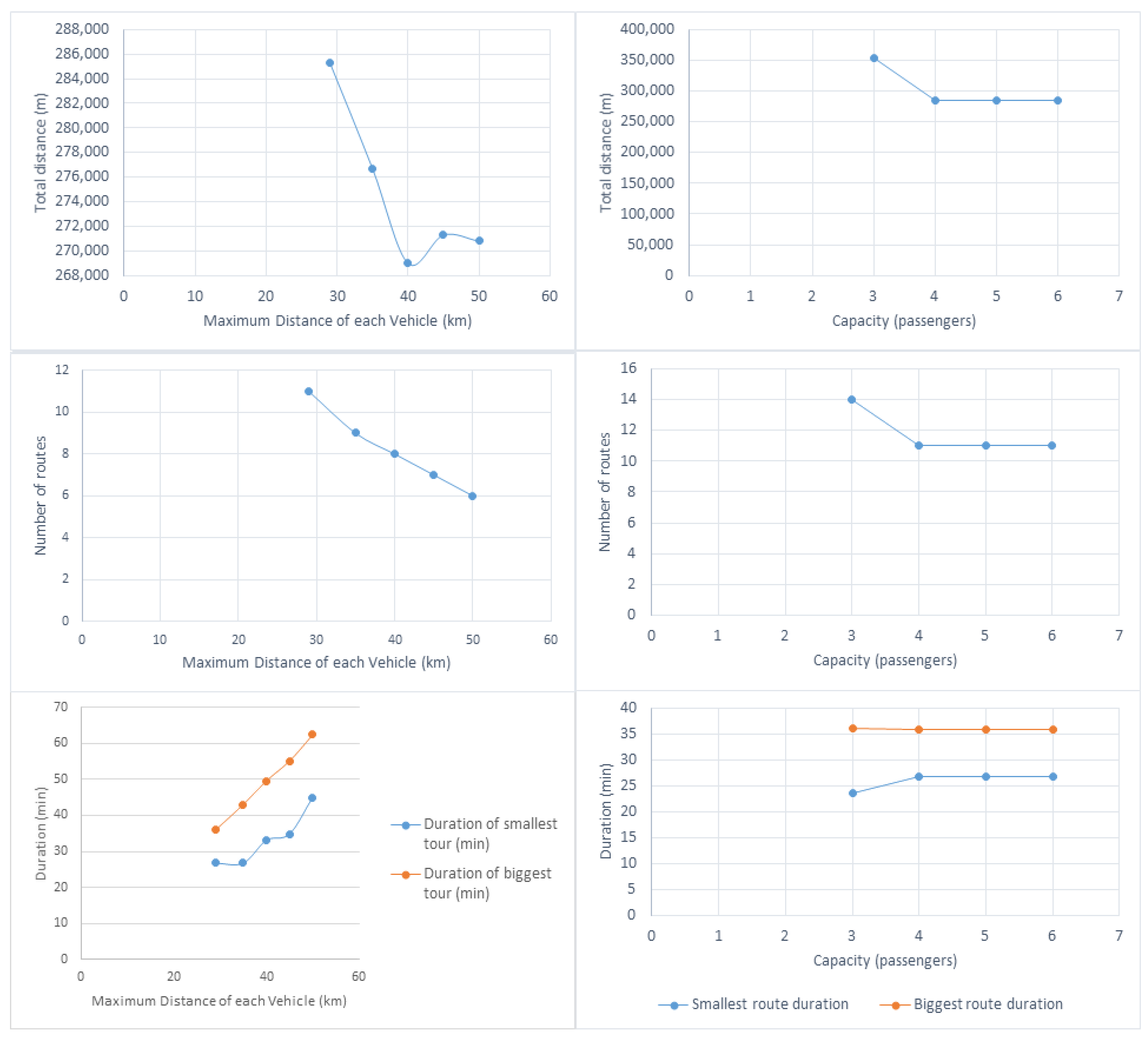
A sensitivity analysis for the vehicle range, capacity and passenger demand is performed to investigate algorithm robustness. Tests are conducted for maximum range values of 35, 40, 45 and 50 kilometers and for vehicle capacity values ranging from 3 to 6 passengers. Passenger demand variations within +/− 20% and +/− 50% were examined. The results for the range and capacity constraints are shown in Figure 6.

As expected, increasing maximum vehicle range leads to a reduction in the total distance traveled by vehicles, as it allows for the creation of more efficient routes, reducing total distance by roughly 6%. However, as shown in Figure 6, when vehicle range increases beyond a certain threshold, objective function values begin to rise due to vehicles wasting too much time as they move from point to point within the road network. Reasonably, increasing maximum vehicle range also leads to a reduction in the number of routes, as vehicles can serve more passengers before returning to their depot.

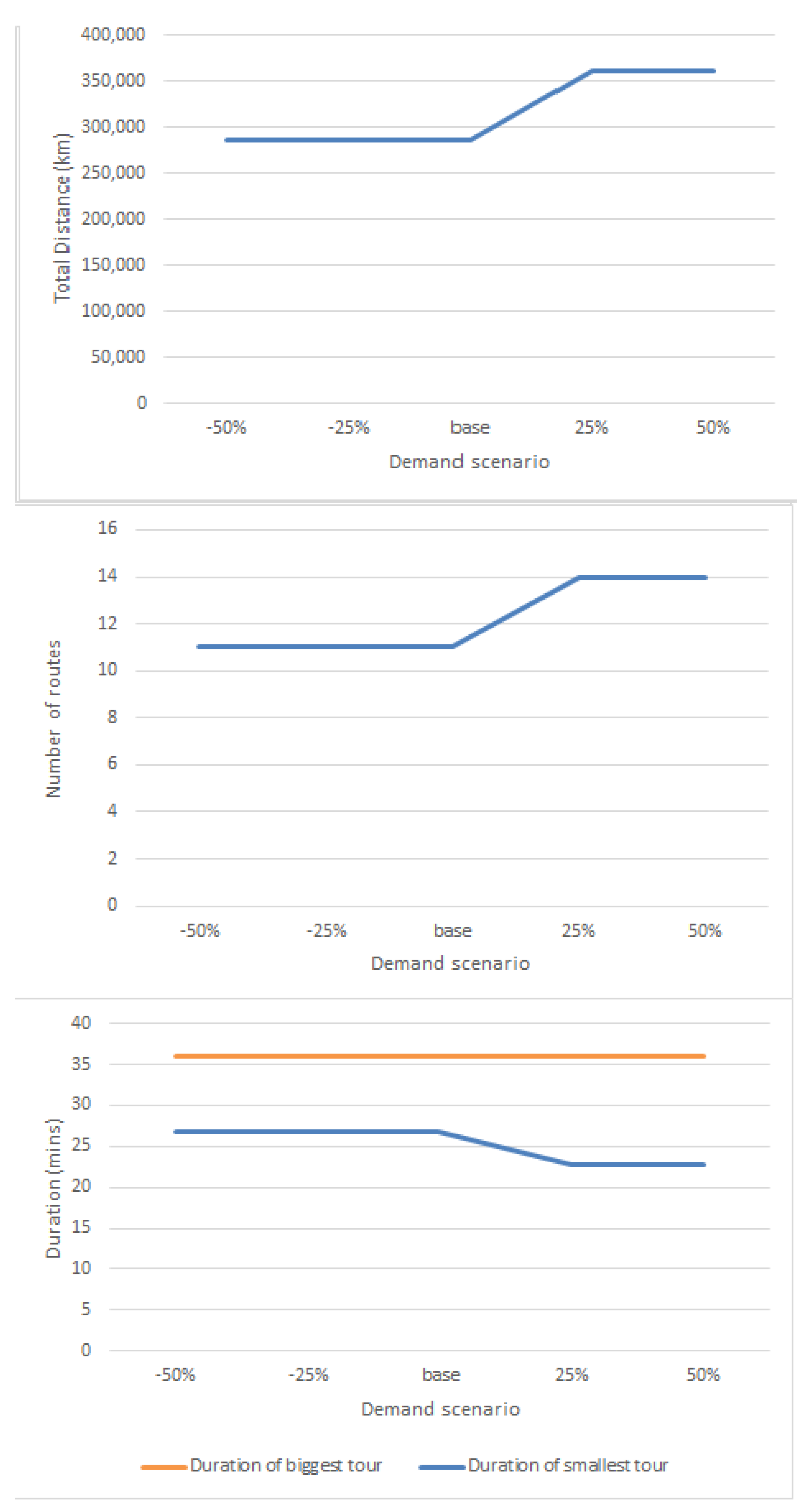
As expected, increasing vehicle capacity reduces both the objective function values and the number of required routes. In contrast, restricting the maximum capacity to three leads to a total distance value of 350 km, a 24% increase from 285.3 km, which is the result for the capacity values of four, five and six. Furthermore, 14 total routes are needed when the capacity is set to three, while 11 routes are needed with a capacity of four, five and six passengers. This occurs because each vehicle can serve a higher number of customers with the increased capacity. Time durations for the largest and smallest route are also investigated. As expected, increasing maximum vehicle range results in higher travel times, while an almost linear pattern may be observed in that case. As a general note, average travel times increase for higher capacity values, as travel times for the smallest routes increase while durations for the biggest routes remain virtually unchanged. However, maximum range constraints restrict travel times up to a certain limit. We also examined values corresponding to −50%, −25%, +25% and +50% compared with the initial demand. Due to capacity constraints, values exceeding capacity are rounded to the maximum allowed value. Accordingly, values under unity are rounded to one. Results are shown in Figure 7.

4. Discussion

Emerging forms of shared mobility call for new formulations for the VRP, taking into account vehicle sharing, ride sharing and autonomous vehicle fleets. This study considers a many-to-many customer demand, vehicle operational constraints and, also, the possibility of shared rides among passengers with different origins and destinations. An ant colony optimization algorithm was employed to solve the relevant problem, which was appropriately modified to handle ride sharing and vehicle range constraints. A targeted insertion operator was employed to exploit the possibility of shared rides among passengers with different origins/destinations while not imposing excessive detours on them. The algorithm was applied to a set of points within Athens (Greece) in areas where demand is expected to be high in an effort to realistically model the problem. Findings indicate that the optimized routes serve all customer requests with a relatively small number of vehicles, taking into account the strict constraint of maximum vehicle range that is imposed.

The performance of the algorithm was robust, as demonstrated through a series of experiments. Sensitivity analysis showed that restricting capacity to just three passengers can lead to more expensive solutions, e.g., a 24% increase in the objective function and a 27% increase in the number of routes, whereas increasing the SAV range to 40 km can reduce distance costs by approximately 6%. Demand variations, on the other hand, did not affect results too much due to capacity constraints.

All in all, results underline the potential of exploiting shared autonomous vehicles in the context of a taxi service for booking trips through electronic reservation systems. This work considered a static setting, intended at designing a service for regular micro-transit commuters. Further research directions include modifying the algorithm to address more complex operating conditions such as time windows and dynamic demand and travel times. For instance, heterogeneous fleet considerations and indicators related to the fairness and efficiency of ride-sharing operations [30] may be integrated into similar problems. Furthermore, in this study, a maximum number of available vehicles was considered that was enough for all customers to be served. Future studies, however, may set a smaller number of available vehicles without requiring that all requests must be served. Last, linearization techniques may be exploited to reduce problem complexity for non-linear formulations and to improve the efficiency of solving small/medium-sized cases [47,48].