Velocity Prediction Based on Map Data for Optimal Control of Electrified Vehicles Using Recurrent Neural Networks (LSTM)

Abstract

In order to improve the efficiency of electrified vehicle drives, various predictive energy management strategies (driving strategies) have been developed. This article presents the extension of a generic prediction approach already proposed in a previous paper, which allows a robust forecasting of all traction torque-relevant variables for such strategies. The extension primarily includes the proper utilization of map data in the case of an a priori known route. Approaches from Artificial Intelligence (AI) have proven to be effective for such proposals. With regard to this, Recurrent Neural Networks (RNN) are to be preferred over Feed-Forward Neural Networks (FNN). First, preprocessing is described in detail including a wide overview of both calculating the relevant quantities from global navigation satellite system (GNSS) data in several steps and matching these with data from the chosen map provider. Next, an RNN including Long Short-Term Memory (LSTM) cells in an Encoder–Decoder configuration and a regular FNN are trained and applied. The models are used to forecast real driving profiles over different time horizons, both including and excluding map data in the model. Afterwards, a comparison is presented, including a quantitative and a qualitative analysis. The accuracy of the predictions is therefore assessed using Root Mean Square Error (RMSE) computations and analyses in the time domain. The results show a significant improvement in velocity prediction with LSTMs including map data.

1. Introduction

In recent years, many alternative propulsion systems have been developed. This includes both pure electric and hybrid electric vehicles (HEVs). Electrified drives are characterized by component dimensioning, topology, and driving strategy [1]. The latter must guarantee that the system functions are used optimally under various driving conditions. The studies [2,3,4,5,6] provide a comprehensive summary of the current state of research in this sector, whereby predictive driving strategies are being widely examined. Here, information about the upcoming driving profile is considered in the propulsion control through related algorithms to achieve additional fuel savings [7]. This includes, for example, future torque and power requirements. In general, there are a variety of sources that may be used to forecast such future torque demand. Telemetry data from the Global Navigation Satellite System (GNSS), Car-to-Car (C2C), and Car-to-X (C2X) should be mentioned. In addition, information from Radar, Lidar, and cameras may be used to make predictions. These communication units and sensors, on the other hand, are not mandatory, and the constant availability of such data cannot be guaranteed for reliable on-road forecasts. As a result, researchers in [8] present a generic prediction model based on AI that ensures a reliable forecast of future torque demand without the need for any telemetry data. Hereby, past driving profiles are sufficient to train the model. For forecasting, the model simply needs to know the previous and present conditions of the current trip.

In the context of this paper, the presented investigations from [8] regarding the application of predicting torque-relevant variables are extended. Therefore, RNNs with Long Short-Term Memory cells (LSTMs) are applied in an architecture developed for the proposed application, including an Encoder–Decoder configuration. It is further shown how map data can lead to an improvement of velocity prediction accuracy, when the case of both a known trip and the availability of map data for the current GNSS position arises. This is the case, for example, when entering the route in the navigation system or by traveling a known route again, which is detected by intelligent algorithms. Overall, the goal remains to attain a robust application of the whole generic prediction approach including the proposed extension.

2. Related Work

Vehicle velocity is a complex function of environmental conditions, the vehicle, and the driver [9,10]. Therefore, at first, major influences on the driving profile are introduced. In a further step, a deeper look into existing velocity prediction methodologies is given through corresponding publications.

Today’s vehicles vary widely in type and cover a wide range of performances. As shown by [11], significantly different average velocities can be observed depending on the vehicle type under the same conditions. In particular, a clear downward trend in vehicle velocity with increasing vehicle age can be seen. Other vehicle-specific characteristics, such as engine size or vehicle load are mentioned. Another factor is the behaviour of the driver [12]. According to [13], demographic characteristics such as the age and gender of the driver, as well as the character and current mood of the person driving are decisive here. [14] also suggests an influence of the driver’s subjective perception regarding the quality of the road. The infrastructure imposes external constraints on the driver through legal requirements or driving recommendations, which thus significantly influence the velocity profile of a route [15]. According to [16], traffic lights and intersections are crucial here. Speed limits also play a decisive role. Natural environmental conditions such as weather, time of day, or light conditions also matter. Researchers in [13] suggest a crucial difference between day and night driving. Another important category is influences related to the road itself. Not only the road surface, but also the shape and curvature have a relevant influence on the velocity profile [17]. Particularly in curves, the limiting factor is usually not the maximum permitted velocity, but the maximum lateral acceleration accepted by the driver. Road slope can also have a non-negligible effect, especially when driving uphill. Researchers in [16,18] assign a high relevance to the consideration of curves, especially for urban driving. Traffic is generally a very dynamic and difficult to predict system as it is highly influenced by other road users. A schematic overview of the influences is provided as an Ishikawa diagram, see Figure 1.

It turns out that the consideration of all information through corresponding prediction models is very difficult. Map data can be used to identify static traffic events such as the position of traffic lights or stop signs. In addition, so-called Live Maps can provide time-dependent information such as traffic jams and traffic densities. Furthermore, the vehicle itself might have on-board sensor systems such as radar systems or cameras to deliver information about the observed traffic, for example, the distance to the vehicle in front [18].

According to [10,12], velocity prediction methodologies can be divided into non-parametric and parametric methodologies.

Parametric Methodologies (PM) are usually based on an analytical function. Examples that fall into this group are: The Constant Speed Model (CS) and the Constant Acceleration Model (CA) [10], but also the so-called Intelligent Driver Model (IDM) [19,20]. The research by [17] describes a possibility of velocity prediction using GNSS data, when the route to be driven is known in advance. To enable such long-term predictions, the route is described as a sequence of traffic events. Based on this, the route is divided into segments of equal maximum velocity. Transitions between the segments are described with acceleration phases or braking phases. Such predictions can be made for the entire route, as they are based only on stationary traffic events. A disadvantage of this method is that it is difficult to take into account spontaneous traffic events such as congestion or temporal variations in traffic density.

Non-parametric Methodologies (NPM) do not require prior knowledge about the exact dynamics of the system. Due to this, they are well suited for modelling systems whose physical foundations are not easy to describe or are even unknown. Furthermore, a robust usage can be ensured, as the route to be driven must not necessarily be known in advance and additional data are not mandatory. Examples are methods from the field of stochastics such as Markov Chains (MC) and data-driven methods such as Artificial Neural Networks (ANN). The generic prediction approach worked out in [8] can be assigned to this category. Moreover, [8] also includes an overview regarding the state of the art for such models. In contrast to PM, NPM cannot be used for velocity prediction of the entire route, but only for short-term predictions.

To sum up, environmental influences including infrastructure, road and traffic, as well as the vehicle and the driver’s behaviour, all play a role in vehicle velocity. In this work, influences accessible by digital maps are of increased interest to predict future vehicle velocity. Moreover, the presented research underlines that data-driven methods from the field of NPM are well suited for the modelling of driving behaviour in a robust application. As already shown in [8], methods from the field of AI should be preferred over MC: It was demonstrated that Feed-Forward Neural Networks (FNN) can achieve 30% more accurate velocity predictions and lead to higher accuracy in total compared to a first-order MC, especially when road slope is considered. However, dynamic changes in the driven profile can only be recognised when they have already been initiated for both MC and FNN. It was concluded that both MC and FNN can predict trends only to a limited extent. In this work, Recurrent Neural Networks (RNN) are used, as they are particularly suitable for time-series predictions and offer improved accuracy compared to FNN. The aim of this work is to demonstrate how the robust prediction approach from [8] can be extended by map data for the case of an a priori known route. It is not intended to replace the approach from [8]. It should be seen as an extension of [8] to additionally increase the prediction accuracy when both map data and GNSS positioning are available. Overall, the aim continues to be to achieve robust applicability of the whole approach. As stated in [8], all traction torque-relevant variables should be predicted to enable the application of Model Predictive Control (MPC). However, in this work, predicting the velocity profile is sufficient, as road slope can be determined from map data for the a priori known route. Acceleration is derived by numerical differentiation from the velocity profile.

3. Method

The methodology outlined in this paper is divided into two main steps. The first main step is preprocessing. This is divided into five substeps:

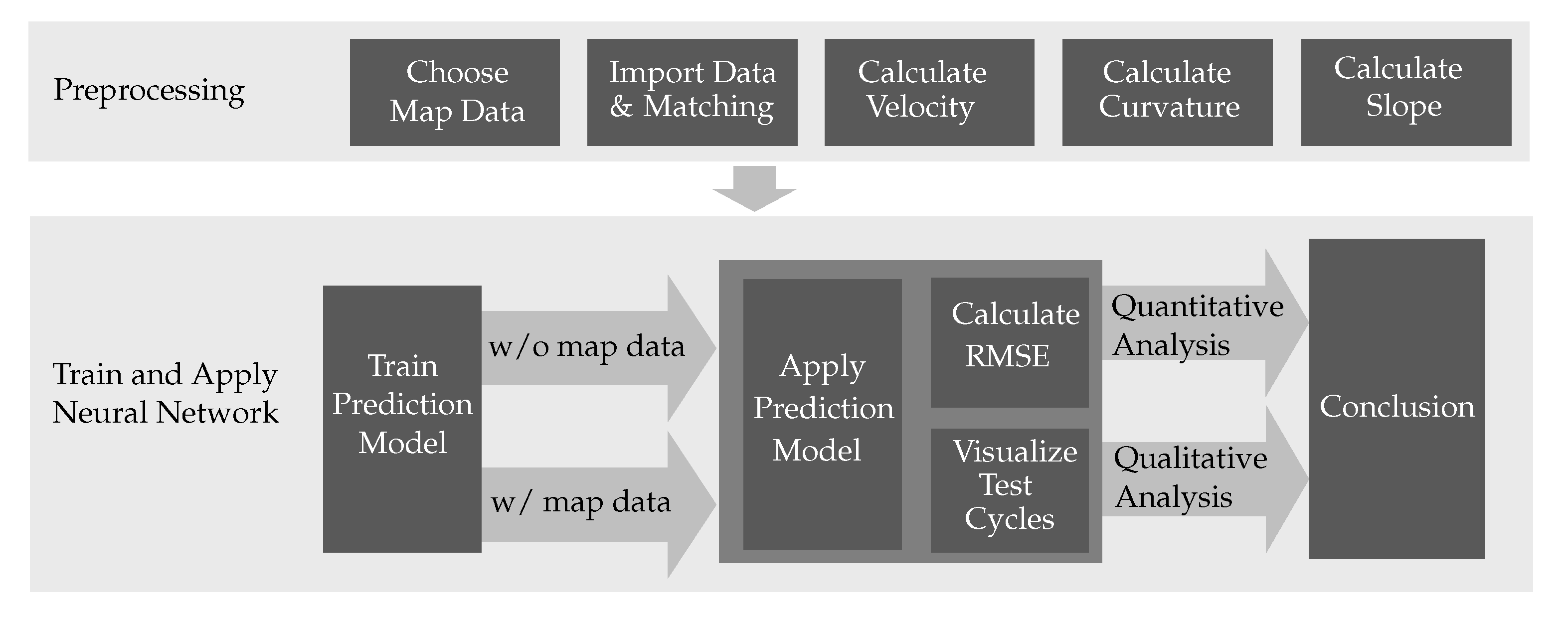
• Choosing a map data source
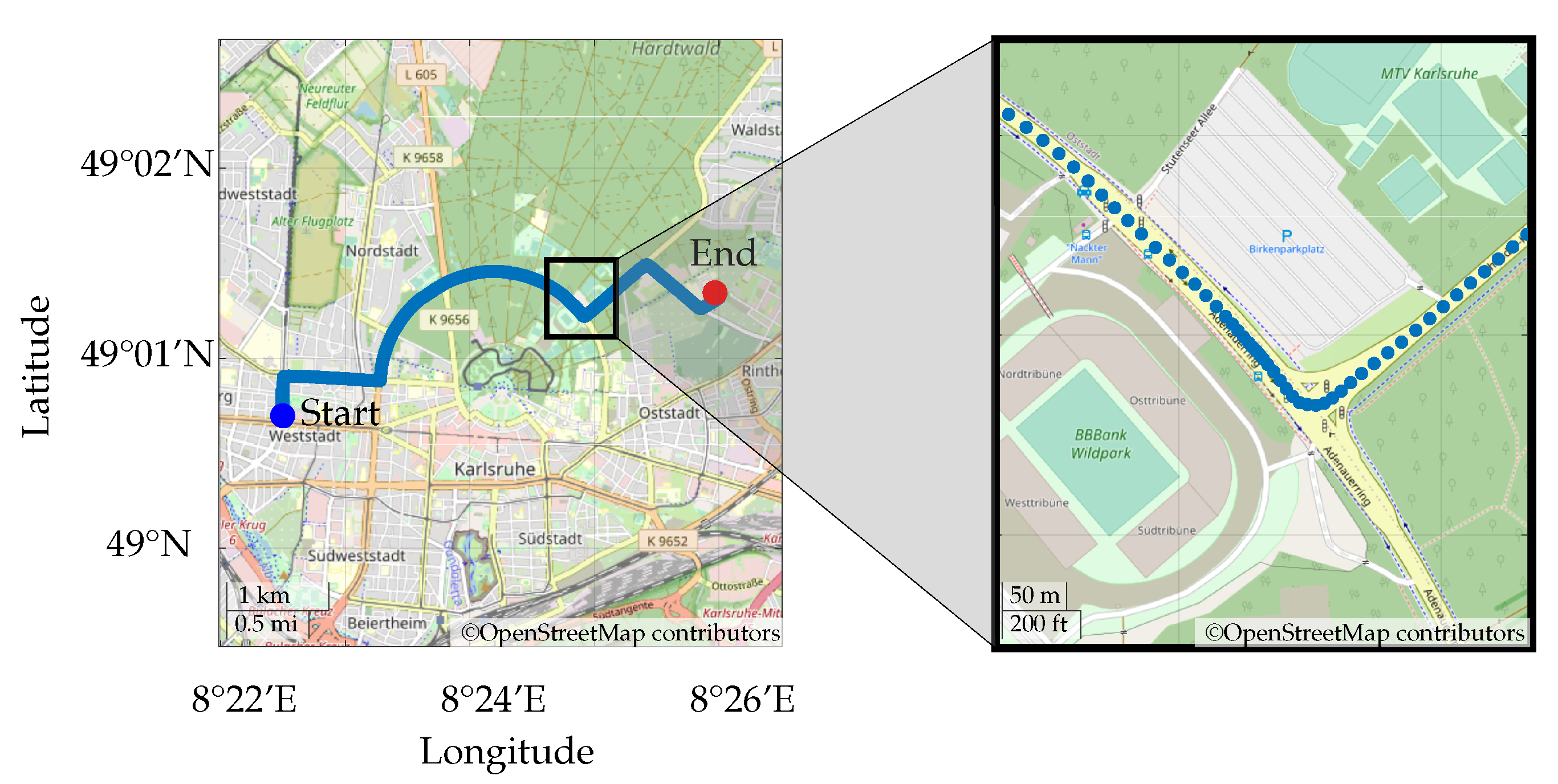
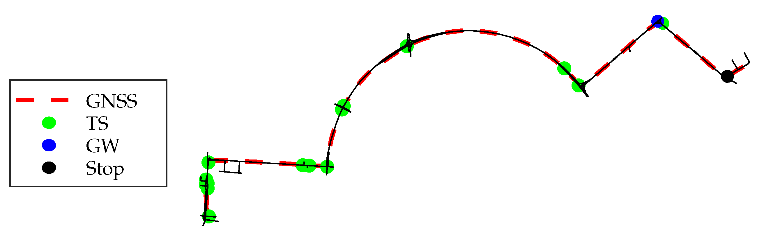
• Importing data from GNSS tracking and matching with map data
• Calculating velocity
• Calculating road curvature
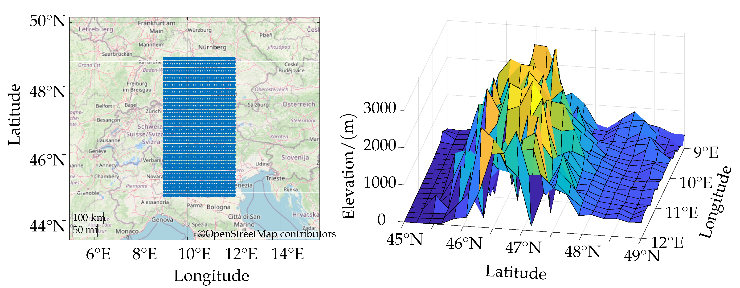
• Calculating road slope

The second main step consists of training and applying the neural network to make predictions over a short horizon (short-term prediction), similarly to [8]. Therefore, the real driving data are first separated into training, validation, and test data at the ratio of 60:20:20. Following this, the ANNs are trained. This includes a model concerning map data and a model without map data. The final evaluation of the results includes both the RMSE values of predicted velocity and acceleration and an analysis of the velocity forecasts in the time domain. The whole procedure is applied both to LSTM and FNN models. The methodology is also summarized in Figure 2.

Investigations from [8] showed that AI should be preferred in the prediction of traction torque-relevant quantities compared to other methods such as MC. Moreover [21] revealed that in the field of AI for such time-series prediction, RNNs are particularly suitable compared to FNN. The basic architecture of an RNN is given by Figure 3 [22]. In the simplest RNN, a so-called Vanilla RNN, the hidden state $h_t$ is calculated using the parameter weights $W_{hh}$, $W_{xh}$, the input $x_t$, and the previously hidden unit $h_{t-1}$. A tanh is used to keep the hidden state $h_t$ between −1 and 1. The output $y_t$ is finally calculated by multiplying the hidden state $h_t$ with another parameter weight $W_{hy}$ [23,24].

$$h_t=tanh(W_{hh}{h}_{t-1}+W_{xh}{x}_t)$$

(1)

$$y_t=W_{hy}{h}_t$$

(2)

Further information regarding RNNs can be found in [25,26,27,28]. Basic RNNs have problems in considering long-term dependencies. For this reason, [29] introduced the Long Short-Term Memory (LSTM). In contrast to basic RNNs, besides the hidden state $h_t$, an LSTM includes a cell state $C_t$. The cell state can be seen as a long-term memory of the model. In contrast to a Vanilla RNN, an LSTM includes two types of activation functions; tanh and sigmoid. Tanh, similarly to Vanilla RNN, limits the dataflow to values in between −1 and 1. Sigmoid determines whether to update or forget certain data (limits to values between 0 and 1). An overview of an LSTM cell is given in Figure 4. The different parts of a basic LSTM should be introduced shortly in the following [23,24,30,31,32,33].

Based on the previous hidden state $h_{t-1}$ and the current state $x_t$, the forget gate output $f_t$ is calculated using a sigmoid function. This aims to keep or forget information from previous cell state $C_{t-1}$. Next, new information is stored in the cell state. Therefore, an input gate is used. It consists of a sigmoid layer which decides which values to update (input gate output $i_t$) and a tanh layer, which determines new candidate values $\widetilde{C_t}$. The new cell state $C_t$ is calculated using the forget gate output $f_t$, the old cell state $C_{t-1}$, the input gate output $i_t$, and the new candidate values $\widetilde{C_t}$.

$$C_t=f_t·C_{t-1}+i_t·\widetilde{C_t}$$

(3)

The output $o_t$ of the Output Gate is calculated by passing both the previously hidden state $h_{t-1}$ and the current input $x_t$ through a sigmoid function. Furthermore, the new cell state $C_t$ is applied to a tanh function. The current hidden state $h_t$ is finally calculated by multiplication as follows.

$$h_t=o_t·tanh\left(C_t\right)$$

(4)

It should be noted that not all LSTMs are equal. A popular version of an LSTM including so-called peephole connections, for example, was introduced by [34]. Apart from that, there are LSTM modifications without the output gate called Gated Recurrent Unit (GRU) [35].

4. Implementation

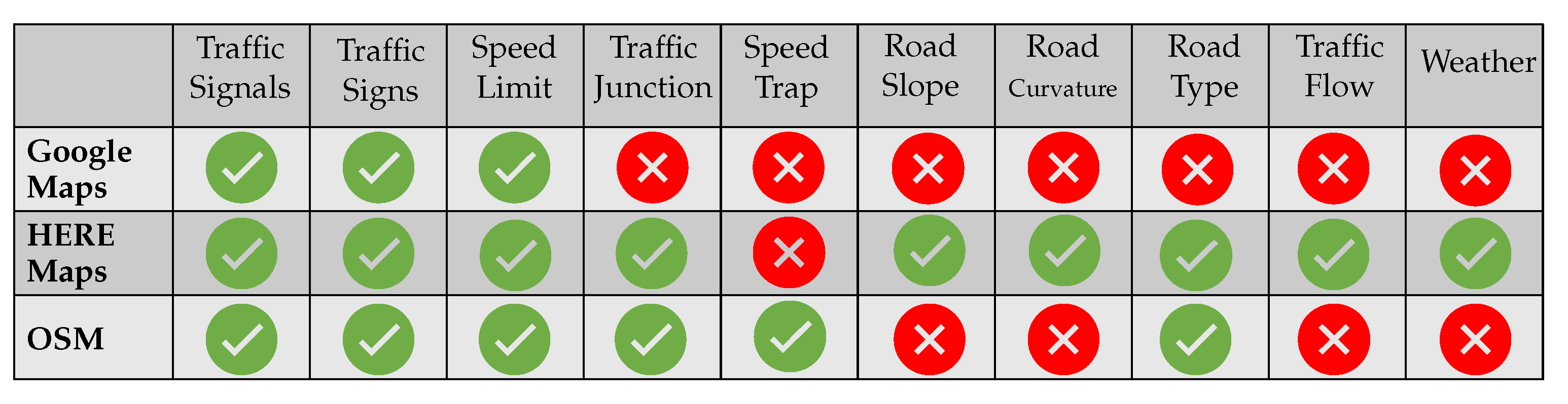
4.1. Choosing Data Sources

In Figure 1, different influences on the driving profile were identified through analysis of related work. However, as already stated earlier, the focus of this paper is on information provided from map data. Therefore, the road slope, the legal speed limit, the curvature, traffic signals, stop- and give way signs are determined for predictions. Three providers of relevant data are investigated in the following, a selection is made based on the following criteria.

• Available map data and road attributes
• Cost of use of the provider (free availability is to be aimed at)
• Quality of the data (accuracy, completeness, up-to-dateness)
• Effort of data processing

Google Maps is supposed to provide very up-to-date and accurate data [36]. However, the service is limited for private users, especially in the case of free application. HERE provides a larger selection of road attributes, and data are also considered to be both up-to-date and accurate [37]. However, HERE also has the problem of limited usability due to a limit on the number of calls per time. Compared to the other two providers, Open Street Map (OSM) has the advantage that it can be used free of charge without restriction. This includes a wide range of both infrastructure data and road attributes. However, certain data, such as current traffic data, cannot be taken from the database. An overview of the available infrastructure data of the individual providers can be found in Figure 5.

Regarding the criteria listed above, OSM is chosen as an appropriate solution. Numerous uses of OSM in an academic setting demonstrate a sufficient accuracy and reliability of the data. An example of this is an application for localization using OSM by [38]. A study on a quality assessment of OSM data is provided by [39]. Research by [40] suggests a major influence of road slope. However, OSM does not have sufficient coverage of the map with elevation data. Therefore, data are enriched with elevation data provided by Shuttle Radar Topography Mission (SRTM). SRTM data are remote sensing data of the Earth’s surface, which were conducted in 2000 by the National Aeronautics and Space Administration (NASA). It has a resolution of one arc second and covers almost all important land areas on Earth. The resolution of one arc second corresponds to a grid constant of about 30 m (depending on the latitude).

4.2. Importing Data Including Matching

In [8] a comprehensive dataset, which includes 4500 km of real driving cycles, was already discussed in detail. It includes four different drivers and covers the entire spectrum from city driving, to country road driving, through to highway driving. In a first step of this work, a selection of the driving data of various test drivers is imported. The data were tracked at a constant rate of 1 s as can be seen in Figure 6: A reduction of velocity, for example in a curve, leads to the tracking points becoming significantly closer.

In a next step, relevant OpenStreetMap (OSM) data are downloaded from Geofabrik [41]. After reducing data using Osmosis [42], further preprosssing is performed with two Matlab functions called xml2struct [43] and parse_openstreetmap [44]. Finally, two Matlab structs are available. One struct includes nodes, fetched from OSM. Nodes are points of interest, which are defined by their coordinates, the specific attributes of the node (for example whether a traffic signal is there), and an individual ID. Nodes are further assigned to so-called ways, which represent the second struct. Ways can be interpreted as streets, which can also have specific attributes, such as legal speed limits. In a next step, elevation data of SRTM are downloaded from [45]. The data are visualized in Figure 7, where the alps can be seen clearly. Furthermore, e.g., the elevation around venezia at sea level (12 °E, 45 °N) and the swabian alps, at a height of around 800 m at 9.5 °E, 48.5 °N can be identified clearly.

While the enrichment with SRTM elevation data is achieved by a simple 2D interpolation, a challenge lies in the efficient matching of the GNSS tracks with the relevant data from the OSM structs. For this, the data-driven method KDTreeSearcher from Matlab is used. In Figure 8, the route already presented in Figure 6 is plotted including the streets considered by the developed matching algorithm (black lines). Furthermore, the identified nodes from traffic signals (TS, green points), give way (GW, blue points), and stop (black points) are marked.

Additionally, the legal speed limit is appropriately detected, even when it is sensitive to the direction.

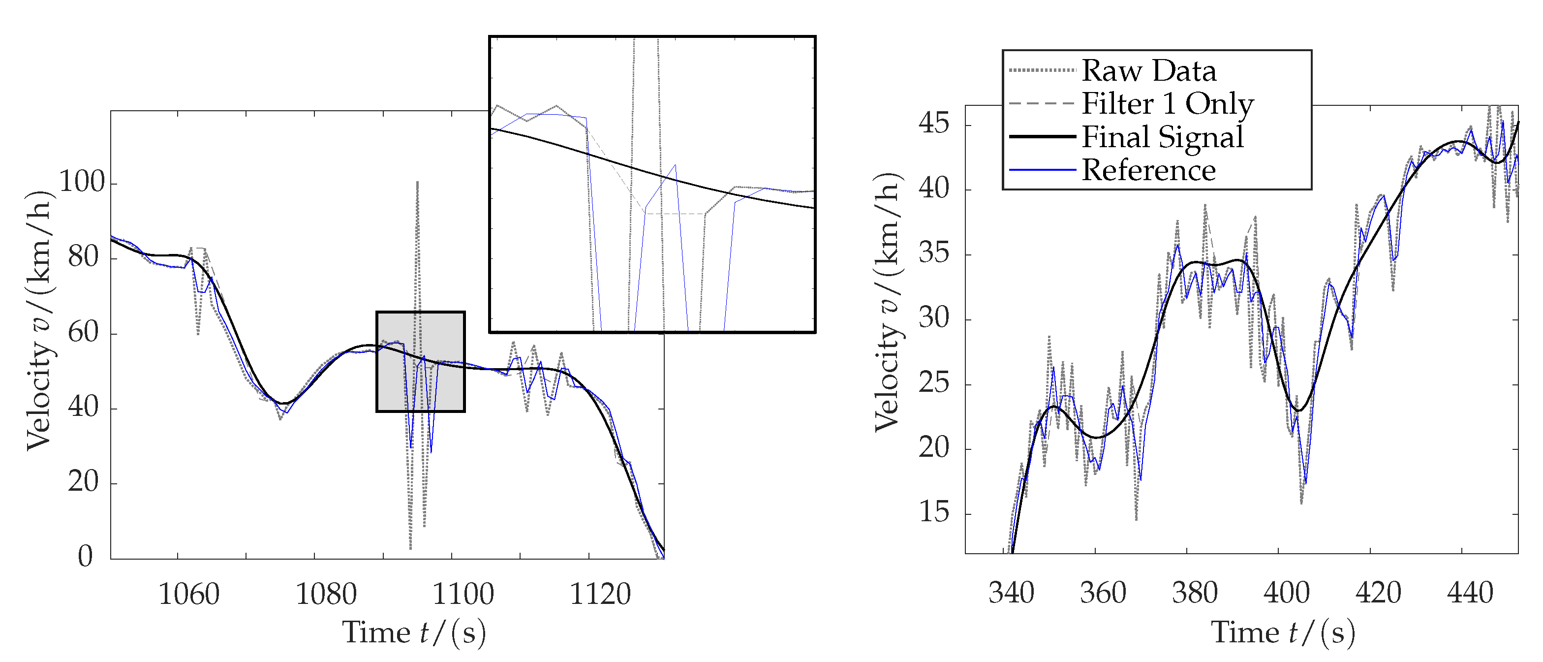
4.3. Calculating Velocity

To ensure a robust velocity calculation from the GNSS tracks, a two-step filter methodology is developed: In the first step, a maximum acceleration and deceleration are defined for the individual test vehicle used on the basis of [46], which are stored in a lookup table as a function of the velocity. Incorrect measurements resulting from a jump in the GNSS signal (see Raw Data) are then overwritten using a linear interpolation between the first and last valid data points (see Filter 1 Only). In the second step, a lowpass filter is used to calculate the Final Signal. The optimal normalized passband frequency is found through an RMSE comparison between final signal and reference signal (Reference). This reference velocity is calculated independently using an alternative calculation. The effects on two exemplary sequences are presented in Figure 9.

As can be seen in Figure 9, obvious outliers can be well corrected with the first filter, (see Filter 1 Only signal in plot on the left). Further filtering with the low-pass filter eliminates high-frequency disturbances (see Final Signal on the right). However, the plot on the left especially reveals that the reference signal is also biased and therefore only provides limited information.

4.4. Calculating Road Curvature

Various approaches to calculating curvature have been worked out during the last years. For example, it can be assumed that the vehicle moves between three points of the GNSS track on a circle section. By knowing the position of the current point, the coordinates of the point at time $t_{t-1}$ and the next point $t_{t+1}$, the radius of the assumed circle at time $t_t$ can be calculated. However, the results with this simple geometric approach are not satisfactory due to inaccuracies in the GNSS measurements.

To ensure robust use, another two-step filter methodology is applied: In the first step, the path is smoothed by use of smoothPathSpline from Matlab Automated Driving Toolbox which smoothens the vehicle path using cubic spline interpolation and therefore calculates new data points with a constant distance. In the second step, the bearing $\varphi$ is calculated to a specified axis for each timestep, which is finally filtered again by a low-pass filter, similar to Section 4.3. Finally, the curvature is calculated using $\kappa =\frac{d\varphi }{ds}$, whereby $d\varphi$ represents the change of bearing to the specified axis, and $ds$ stands for the corresponding path section of the track.

For validation, the proposed algorithm is applied to the exemplary driving cycle which has already been presented in Figure 6. The goal is to determine the radius of the Adenauerring in Karlsruhe, Germany by using the proposed algorithm (see Figure 10).

In the left plot of Figure 10, both the Raw Data and the Smoothed Data of the GNSS data can be seen. A radius of 1125 m can be calculated through cycle approximation. In the right plot, the calculated bearing signal is plotted, both with the low-pass filter (black line) and without (grey line). Furthermore, final curvatures are presented (red line). A ${\mathrm{\Delta }}_{bearing}$≈ 150° over a distance of d ≈ 2600 m can be estimated roughly from the right plot, which in turn leads to a radius R ≈ 1000 m. It can be concluded that there is a ≈ 10% deviation from the proposed bearing algorithm. As only a curve detection without any further quantification of the exact curvature is considered in this work, the authors define the proposed algorithm as sufficient. Finally, a suitable threshold is defined. When it is exceeded by curvature $\kappa$, a significant influence on velocity can be expected and a curve flag is output by the curvature algorithm.

4.5. Calculating Road Slope

For the calculation of road slope, a two-step filter methodology is also applied to the elevation signal resulting from interpolated SRTM data (see Section 4.2), visualized by a black dotted line in Figure 11.

In a first step, a filter for detecting and eliminating small jumps in the Elevation Raw signal is used to reduce oscillations in the microscopic range. This can be seen when comparing the black dotted line from the raw signal (Elevation Raw) to the black solid line (Elevation Filtered) in the zoom plots of Figure 11 (bottom). Macroscopic fluctuations, which sometimes extend over several kilometres as in the case of Landecker Tunnel, Austria (see map in Figure 11), however, cannot be reliably detected and eliminated.

In such a case, the SRTM data represent the actual height of the mountain passed through, but not the height of the actual road. Apart from this, there are no measurements in the tunnel itself. As a result, the black dotted line (Elevation Raw signal) at 375 km rises to about 940 m when entering the tunnel. From there, it is interpolated to the next measured GNSS point at the end of the tunnel (750 m at 380 km). As such big jumps cannot be handled properly by the proposed filter algorithm, see black solid line (Elevation Filtered), the Elevation Reference signal, represented by a blue line, is used for further calculations in this work.

Hereby, in a second step, according to [47], a Butterworth filter is applied to the Elevation Reference measurement. Lastly, the slope is calculated from the filtered elevation signal (see Calc. Slope). For validation of the algorithm, both final elevation and slope data for the driven alp-crossing route are compared to literature data.

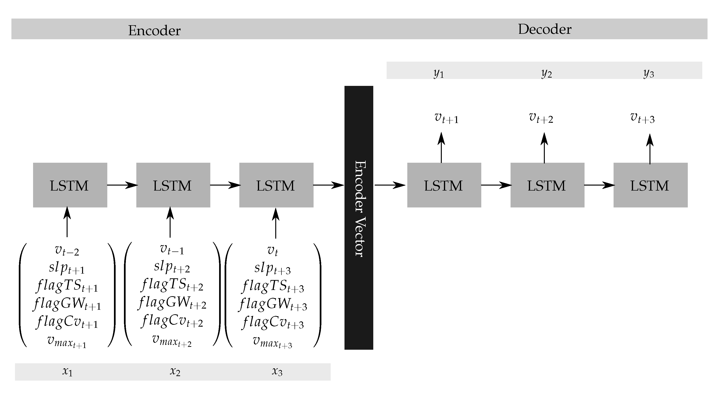
4.6. Short Range Predictions

As already stated, investigations by [8] revealed that AI should be preferred over other approaches such as MC for the prediction of traction torque. Therefore, in Section 3, the basics of RNN and LSTMs were introduced which are particularly interesting for timeseries predictions. In this work an Encoder–Decoder LSTM (from now on called ED-LSTM) is implemented for multivariate, multi-step time series forecasting using Keras. Keras is a TensorFlow platform-based neural network library. Multivariate means that multiple variables are collected as input for the analysis. Multi-step means that several timesteps are to be predicted. Using an Encoder–Decoder configuration enables the opportunity to apply sequences of varying lengths to one another. This can be of benefit, when considering a longer horizon in the input than that of the actual prediction output. An ED-LSTM consists of three components: encoder, intermediate vector, and decoder. Both the encoder and decoder contain several LSTMs. The encoder reads the input sequence and summarizes the hidden state and cell-state information. The encoder’s output is a fixed-length vector that indicates how the model interprets the sequence. The first cell of the decoder network receives the vector from the encoder’s final cell. For each time step, it finally calculates the output $y_t$ [21,48,49]. A simplified scheme of the applied ED-LSTM for multivariate, multi-step time-series forecasting can be seen in Figure 12.

For the input data, every state consists of both several velocity steps from the past and future infrastructure data. The output is defined by future velocity steps. Within the framework of the modelling, it is assumed that the last known velocities in combination with the future route information enable the best possible determination of the future velocity profile. As stated, the lengths of the inputs and outputs can also be different when ED-LSTMs are applied. In the context of this work, however, inputs have the same lengths as outputs. In other words, for a 10 s prediction into the future, past velocity values of a 10 s timespan are chosen. An appropriate amount for the LSTM units is determined through parameter studies, which are not further discussed at this point. In this work, the number of units is set according to the number of timesteps $N_{timesteps,predhorizon}$ to be predicted. Furthermore, similar to FNN, an activation function is needed, whereby the Rectified Linear Unit (ReLu) is chosen. As a Loss function, the Mean Squared Error (MSE) is calculated. The final parametrization including Learning Rate, Batch Size, Epochs, and chosen optimizer can be seen in

Table 1. Parameters for RNN for 10 s prediction.

LSTM Units	$N_{timesteps,predhorizon}$
Optimizer	Adam
Loss Function	Mean Squared Error (MSE)
Activation Function	Rectified Linear Unit (ReLU)
Learning Rate	0.01
Batch Size	1400
Epochs	1000

.

The parameterization of the FNN has already been discussed in detail in [8] and has been adopted for this work. However, the number of inputs is increased by the number of variables to be considered. With a 10 s prediction and 5 variables from map data, for example, the architecture of the FNN consists of 60 inputs. In contrast to LSTM, the time order and a separation of the different variables are not included in the model architecture of the FNN.

5. Results

Preprocessing including all applied substeps is already discussed in detail in the explanations about implementation (Section 4). Therefore, the following statements are limited to the quantitative and qualitative analyses of the results from ED-LSTM and FNN. In terms of calculating the optimal control for an HEV, the crank torque is needed, which can be calculated from the wheel torque taking into consideration the wheel radius as well as the gearbox ratios. The wheel torque, in turn, is impacted by vehicle-specific parameters and driving cycle-specific variables such as velocity, acceleration, and road slope [8]. As road slope is known for a given route from the start of the trip, this variable will not be analyzed. Accordingly, the analysis focuses on the predictions of velocity and acceleration.

5.1. Analysis of RMSE Values (Quantitative Analysis)

Table 2. RMSE without map data for different prediction horizons.

		Horizon 10 s		Horizon 20 s		Horizon 30 s
		ED-LSTM	FNN	ED-LSTM	FNN	ED-LSTM	FNN
$RMS{E}_v$	$\mathrm{k}\mathrm{m}/\mathrm{h}$	6.43	7.74	12.23	14.10	16.44	17.84
$RMS{E}_a$	$\mathrm{m}/{\mathrm{s}}^2$	0.52	0.57	0.59	0.62	0.65	0.66

and

Table 3. RMSE with map data for different prediction horizons.

		Horizon 10 s		Horizon 20 s		Horizon 30 s
		ED-LSTM	FNN	ED-LSTM	FNN	ED-LSTM	FNN
$RMS{E}_v$	$\mathrm{k}\mathrm{m}/\mathrm{h}$	5.33	6.46	5.77	9.29	10.31	11.82
$RMS{E}_a$	$\mathrm{m}/{\mathrm{s}}^2$	0.48	0.52	0.49	0.56	0.58	0.60

show the RMSE values between actual profile and predicted profile for three different prediction horizons (10 s, 20 s, and 30 s). This includes velocity ($RMS{E}_v$) and acceleration ($RMS{E}_a$). A direct comparison was also made with FNN, which was already presented in [8]. Table 2 lists the predictions without taking map data into account. Here, both ED-LSTM and FNN were trained on the velocity profiles only, on the lines of the explanations from [8]. In contrast to Table 2, in Table 3, the infrastructure data were taken into account, similar to Figure 12.

Comparing Table 2 (without map data) and Table 3 (with map data) reveals that ED-LSTMs always deliver better results than FNN. This statement is valid for all prediction horizons examined, both for the RMSE values of velocity $RMS{E}_v$ and acceleration $RMS{E}_a$. This observation is in line with the generally known statement that ED-LSTMs deliver better results for time-series predictions. In addition, it can be seen that lower RMSE can be achieved at all times when using map data (Table 3).

Looking in detail, it is revealed that improvements of the $RMS{E}_v$ for ED-LSTMs compared to the application of FNN when using a 10 s prediction horizon are at around 10%. (7.74 km/h vs. 6.43 km/h). The relative error of the $RMS{E}_v$ for 20 s and 30 s window is similar: 12.23 km/h (ED-LSTM) vs. 14.10 km/h (FNN) and 16.44 km/h (ED-LSTM) vs. 17.84 km/h (FNN). Using map data (Table 3) leads to improvements of about 10% for both ED-LSTM and FNN for the 10 s window of the $RMS{E}_v$: An improvement of 6.43 km/h to 5.33 km/h can be detected for the ED-LSTM, and 7.74 km/h vs. 6.46 km/h for the FNN. For the 20 s window, however, using map data leads to significant improvements of about 40%: $RMS{E}_v$ is reduced from 12.23 km/h to 5.77 km/h for the ED-LSTM. For the FNN, $RMS{E}_v$ reduction is from 14.10 km/h to 9.29 km/h. For the 30 s horizon, a similar improvement can be seen. The observed $RMS{E}_a$ values always correlate with the $RMS{E}_v$ values.

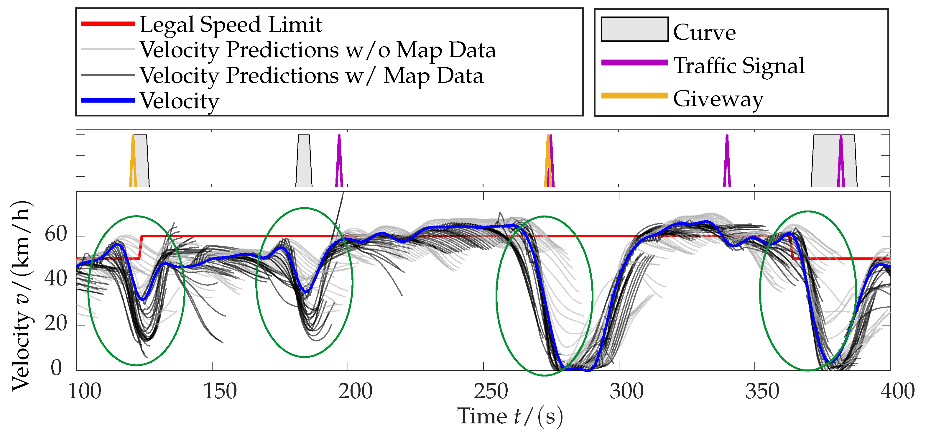
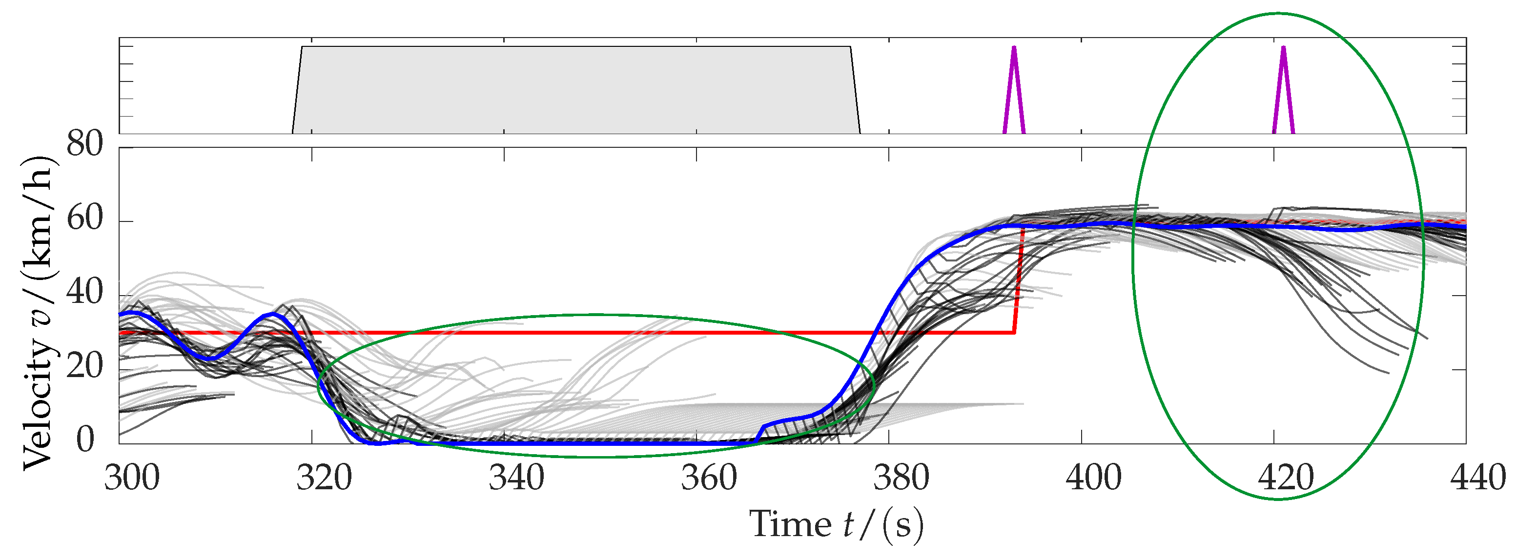
5.2. Analysis in Time Domain (Qualitative Analysis)

In Figure 13, (top), the relevant map data are displayed as a flag over time for a section of a given route. According to Figure 12, this includes curves (grey), traffic signals (violet), and give ways (yellow). In addition, in a further plot, the legal speed limit from map data is visualised (red line). Furthermore, the corresponding real driving profile is presented (blue line). The predictions of the ED-LSTM are plotted by a light grey and dark grey line, both for a prediction horizon of 20 s. The predictions in light grey, represent predictions without any knowledge of map data (see Table 2). The predictions in dark grey represent predictions including map data (see Table 3) as presented in Figure 12.

A correlation between the velocity profile-driven (blue line) and the identified map data can be recognised. At t = 120 s, both a give way sign and a curve are detected. Although the vehicle does not stop, the curve causes a significant reduction in velocity to ≈30 km/h. The velocity of the vehicle is also reduced at t = 180 s. However, a stop resulting from the traffic lights at t = 200 s is not recognisable, either. It is unclear whether the velocity reduction results from the curve or from a back-up of the red traffic light, which just turned green again. At t = 340 s, the traffic signal is clearly green and thus has no influence on the velocity profile. At t = 280 s and t = 380 s, there is obviously a stop due to the detected traffic lights.

An analysis of the breaking manoeuvres demonstrates that the ED-LSTM can predict a breaking manoeuvre much more precisely than without knowledge of the map data. This can be seen particularly well in the driving situations at t = 120 s, t = 180 s, t = 280 s, and t = 380 s (green circles). The ED-LSTM without knowledge of the map data predicts a velocity profile without any major dynamics (light grey lines) in all driving situations. The ED-LSTM with knowledge of the map data, on the other hand, predicts an appropriate breaking manoeuvre as soon as the flag has moved into the prediction horizon (20 s). However, unrealistic predictions are also issued in some cases, which are avoided in the ED-LSTM without map data (see t = 130 s). This is because of the higher complexity of the RNN when map data are taken into account. An increase in the training data could provide a solution to this problem.

As visualized in Figure 14, there are also standing phases that cannot be explained directly with map data. From t = 320 s to t = 380 s, there is a standstill in a curve situation. The reason is not clear, however, a tailback from the traffic light at t = 390 s is possible. Clearly, the ED-LSTM with map data predicts the standphase much more accurately than the one without map data. The problem of inaccurate stand phase predictions was already identified as a weakness of the FNN in [8]. Although this weakness also occurs analogously with the ED-LSTMs when no map data are available, the ED-LSTMs taking map data into account seem to predict these situations much better.

Moreover, t = 420 s demonstrates another weakness of the proposed implementation: When a traffic light occurs (420 s), breaking manoeuvres are predicted from t = 410 s on, until the traffic light situation is overcome without breaking. Predictions using the map data are obviously worse than those without using the map data, as can be seen by the corresponding light grey and dark grey predictions. Knowledge about the status of the traffic lights, for example via camera information, could possibly make the predictions much more precise.

It should be considered whether in a further development of the model, instead of the specified time horizon, a specific future distance of x m should be used as input for the ED-LSTM. For implementation in a real vehicle, an assumption regarding upcoming velocity has to be made to transfer the map information from the distance domain to the time domain.

6. Conclusions

It was shown how an existing robust generic approach to the prediction of traction torque-relevant variables can be extended. This extension focuses on the consideration of map information in the case of an a priori known route and the availability of the corresponding GNSS signal.

An analysis of related work revealed that the influences on the driving profile are complex and a consideration in the driver model is challenging. Therefore, the paper focuses on the utilization of Artificial Neural Networks (ANNs). These are particularly suitable for modelling systems whose physical foundations are not easy to describe or are even unknown. At the same time, a robust use can be ensured for the chosen application. Additionally, in the course of the work, map data were added to raise prediction accuracy. The most suitable map data provider was selected based on defined criteria. Next, GNSS tracks were enriched using both Open Street Map (OSM) data and data from the Shuttle Radar Topography Mission (SRTM). Positions of traffic signals, give way signs, and stops as well as maximum legal velocity were identified properly. Furthermore, velocity, road curvature, and road slope were determined. After preprocessing, Long Short-Term Memory (LSTM) cells from the field of Recurrent Neural Networks (RNNs) in an Encoder–Decoder configuration (ED-LSTM) were applied, as they are particularly suitable for time-series predictions. Additionally, a comparison to Feed-Forward Neural networks was given. Both ANNs were applied to the driving profiles and evaluated with regard to their predictive quality: After calibrating the models appropriately, quantitative analyses regarding RMSE values and qualitative analyses in the time domain were successfully performed for each approach. Regarding the quantitative analysis, it became clear that ED-LSTMs consistently outperform FNN. This assertion holds true for all of the prediction horizons investigated and the RMSE values of velocity $RMS{E}_v$ and acceleration $RMS{E}_a$. This finding is consistent with the widely held belief that ED-LSTMs perform better in time-series prediction. Furthermore, it was observed that when employing map data, lower RMSE values are reached at all times. From the qualitative analyses of the ED-LSTM, it could be confirmed that identified map data are considered properly. However, the limits were revealed, for example in the case of a green traffic light.

To summarize, ED-LSTM should be preferred over FNN, and considering map data in the predictions provides additional benefits regarding prediction accuracy. Further work should deal with how the ED-LSTM can be enriched with additional information to make the predictions more precise. The easy expansion allows the use of Radar, Lidar, and camera or additional data from C2C, C2X if these are accessible. This should make it easier to predict standstill phases that cannot be explained by map data or, for example, to predict that a stop will not be made if the traffic light is green. This higher prediction accuracy allows the energy management strategy to optimize more accurately and, thereby, ultimately allows getting closer to the global optimal solution.

References

1. Silvas, E.; Hofman, T.; Murgovski, N.; Etman, P.; Steinbuch, M. Review of Optimization Strategies for System-Level Design in Hybrid Electric Vehicles. IEEE Trans. Veh. Technol. 2017, 66, 57–70. [Google Scholar] [CrossRef]
2. Tran, D.D.; Vafaeipour, M.; El Baghdadi, M.; Barrero, R.; van Mierlo, J.; Hegazy, O. Thorough state-of-the-art analysis of electric and hybrid vehicle powertrains: Topologies and integrated energy management strategies. Renew. Sustain. Energy Rev. 2020, 119, 109596. [Google Scholar] [CrossRef]
3. Serrao, L. A Comparative Analysis of Energy Management Strategies for Hybrid Electric Vehicles. Ph.D. Thesis, Ohio State University, Columbus, OH, USA, 2009. [Google Scholar]
4. Rizzoni, G.; Onori, S. Energy Management of Hybrid Electric Vehicles: 15 years of development at the Ohio State University. Oil Gas Sci. Technol. Rev. D’IFP Energies Nouv. 2015, 70, 41–54. [Google Scholar] [CrossRef] [Green Version]
5. Xu, N.; Kong, Y.; Chu, L.; Ju, H.; Yang, Z.; Xu, Z.; Xu, Z. Towards a Smarter Energy Management System for Hybrid Vehicles: A Comprehensive Review of Control Strategies. Appl. Sci. 2019, 9, 2026. [Google Scholar] [CrossRef] [Green Version]
6. Jiang, Q.; Ossart, F.; Marchand, C. Comparative Study of Real-Time HEV Energy Management Strategies. IEEE Trans. Veh. Technol. 2017, 66, 10875–10888. [Google Scholar] [CrossRef] [Green Version]
7. Markschlaeger, P.; Wahl, H.G.; Weberbauer, F.; Lederer, M. Assistenzsystem für mehr Kraftstoffeffizienz. In Vernetztes Automobil; Siebenpfeiffer, W., Ed.; Springer: Wiesbaden, Germany, 2014; pp. 146–153. [Google Scholar] [CrossRef]
8. Deufel, F.; Gießler, M.; Gauterin, F. A Generic Prediction Approach for Optimal Control of Electrified Vehicles Using Artificial Intelligence. Vehicles 2022, 4, 182–198. [Google Scholar] [CrossRef]
9. Yang, S.; Wang, J.; Xi, J. Leveraging Drivers’ Driving Preferences into Vehicle Speed Prediction Using Oriented Hidden Semi-Markov model. In Proceedings of the 2020 4th CAA International Conference on Vehicular Control and Intelligence (CVCI), Hangzhou, China, 18–20 December 2020; pp. 650–655. [Google Scholar] [CrossRef]
10. Lefevre, S.; Sun, C.; Bajcsy, R.; Laugier, C. Comparison of parametric and non-parametric approaches for vehicle speed prediction. In Proceedings of the 2014 American Control Conference, Portland, OR, USA, 4–6 June 2014; pp. 3494–3499. [Google Scholar] [CrossRef]
11. Omari, B.H.A.; Jafari, A.A. Roles of driver and vehicle characteristics in speed choice along rural highways. Int. J. Eng. Manag. Econ. 2015, 5, 181. [Google Scholar] [CrossRef]
12. Yufang, L.; Mingnuo, C.; Wanzhong, Z. Investigating long–term vehicle speed prediction based on BP–LSTM algorithms. IET Intell. Transp. Syst. 2019, 13, 1281–1290. [Google Scholar] [CrossRef]
13. Quimby, A.; Maycock, G.; Palmer, C.; Buttress, S. The Factors That Influence a Driver’s Choice of Speed—A Questionnaire Study; Transport Research Laboratory: Crowthorne, UK, 1999. [Google Scholar]
14. Sagberg, F. Factors Infuencing Driving Speed; TOI Report 765/2005; Institute of Transport Economics: Oslo, Norway, 2005. [Google Scholar]
15. Laraki, M.; de Nunzio, G.; Thibault, L. Vehicle speed trajectory estimation using road traffic and infrastructure information. In Proceedings of the 2020 IEEE 23rd International Conference on Intelligent Transportation Systems (ITSC), Rhodes, Greece, 20–23 September 2020; pp. 1–7. [Google Scholar] [CrossRef]
16. Hellwig, M.; Ritschel, W. The Predictability of Driving in Typical Traffic Conditions. In Proceedings of the 2020 21st International Conference on Research and Education in Mechatronics (REM), Cracow, Poland, 9–11 December 2020; pp. 1–6. [Google Scholar] [CrossRef]
17. Rezaei, A.; Burl, J.B. Effects of Time Horizon on Model Predictive Control for Hybrid Electric Vehicles. IFAC-PapersOnLine 2015, 48, 252–256. [Google Scholar] [CrossRef]
18. Back, M. Prädiktive Antriebsregelung zum Energieoptimalen Betrieb von Hybridfahrzeugen. Ph.D. Thesis, Karlsruhe Institute of Technology, Karlsruhe, Germany, 2005. [Google Scholar]
19. Liu, L.; Zhu, L.; Yang, D. Modeling and simulation of the car-truck heterogeneous traffic flow based on a nonlinear car-following model. Appl. Math. Comput. 2016, 273, 706–717. [Google Scholar] [CrossRef]
20. Treiber, M.; Hennecke, A.; Helbing, D. Congested traffic states in empirical observations and microscopic simulations. Phys. Rev. E Stat. Phys. Plasmas Fluids Relat. Interdiscip. Top. 2000, 62, 1805–1824. [Google Scholar] [CrossRef] [Green Version]
21. Chandra, R.; Goyal, S.; Gupta, R. Evaluation of Deep Learning Models for Multi-Step Ahead Time Series Prediction. IEEE Access 2021, 9, 83105–83123. [Google Scholar] [CrossRef]
22. LeCun, Y.; Bengio, Y.; Hinton, G. Deep learning. Nature 2015, 521, 436–444. [Google Scholar] [CrossRef] [PubMed]
23. Aggarwal, C.C. Neural Networks and Deep Learning; Springer: Cham, Switzerland, 2018. [Google Scholar] [CrossRef]
24. Li, F.F.; Johnson, J.; Yeung, S. Lecture 10: Recurrent Neural Networks; Stanford University: Stanford, CA, USA, 2017; Available online: http://cs231n.stanford.edu/slides/2017/cs231n{_}2017{_}lecture10.pdf (accessed on 25 March 2022).
25. Werbos, P.J. Generalization of Backpropagation with Application to a Recurrent Gas Market Model. Neural Netw. 1988, 1, 339–356. [Google Scholar]
26. Elman, J. Finding Structure in Time. Cogn. Sci. 1990, 14, 179–211. [Google Scholar] [CrossRef]
27. Goodfellow, I.; Bengio, Y.; Courville, A. Deep Learning; MIT Press: Cambridge, MA, USA, 2016. [Google Scholar]
28. Afshine Amidi and Shervine Amidi. CS 230—Deep Learning; Stanford University: Stanford, CA, USA, 2022; Available online: https://stanford.edu/{~{}}shervine/teaching/cs-230/ (accessed on 10 May 2022).
29. Hochreiter, S.; Schmidhuber, J. Long Short-Term Memory. Neural Comput. 1997, 9, 1735–1780. [Google Scholar] [CrossRef] [PubMed]
30. Phi, M. Illustrated Guide to LSTMs and GRUs: A Step by Step Explanation; Towards Data Science: Toronto, ON, Canada, 2022; Available online: https://towardsdatascience.com/illustrated-guide-to-lstms-and-gru-s-a-step-by-step-explanation-44e9eb85bf21 (accessed on 25 March 2022).
31. Graves, A.; Mohamed, A.R.; Hinton, G. Speech Recognition with Deep Recurrent Neural Networks. 2013. Available online: http://arxiv.org/pdf/1303.5778v1 (accessed on 25 March 2022).
32. Graves, A. Generating Sequences with Recurrent Neural Networks. 2014. Available online: https://arxiv.org/pdf/1308.0850 (accessed on 25 March 2022).
33. Jiang, L.; Hu, G. Day-Ahead Price Forecasting for Electricity Market using Long-Short Term Memory Recurrent Neural Network. In Proceedings of the 2018 15th International Conference on Control, Automation, Robotics and Vision (ICARCV), Singapore, 18–21 November 2018; IEEE: Piscataway, NJ, USA, 2018. [Google Scholar]
34. Gers, F.; Schmidhuber, J. Recurrent Nets that Time and Count. In Proceedings of the IEEE-INNS-ENNS International Joint Conference on Neural Networks. IJCNN 2000. Neural Computing: New Challenges and Perspectives for the New Millennium, Como, Italy, 27 July 2000. [Google Scholar]
35. Nowak, J.; Taspinar, A.; Scherer, R. LSTM Recurrent Neural Networks for Short Text and Sentiment Classiication. In International Conference on Artificial Intelligence and Soft Computing; Springer: Cham, Switzerland, 2017; pp. 553–562. [Google Scholar]
36. Ciepłuch, B.; Jacob, R.; Mooney, P.; Winstanley, A.C. Comparison of the accuracy of OpenStreetMap for Ireland with Google Maps and Bing Maps. In Proceedings of the Ninth International Symposium on Spatial Accuracy Assessment in Natural Resuorces and Enviromental Sciences, Leicester, UK, 20–23 July 2010; University of Leicester: Leicester, UK, 2010; p. 337. [Google Scholar]
37. Cahyono, A.; Angogoro, H. Comparison Study of Crowdsource Geographic Comparison Study of Crowdsource Geographic Information Services for Rural Mapping and Toponym Inventory. In Proceedings of the 1st International Conference on Geography and Education (ICGE 2016), Malang, Indonesia, 29 October 2016; Atlantis Press: Amsterdam, The Netherlands, 2016; pp. 275–282. [Google Scholar]
38. Ruchti, P.; Steder, B.; Ruhnke, M.; Burgard, W. Localization on OpenStreetMap data using a 3D laser scanner. In Proceedings of the 2015 IEEE International Conference on Robotics and Automation (ICRA), Seattle, WA, USA, 26–30 May 2015; pp. 5260–5265. [Google Scholar] [CrossRef]
39. Basiri, A.; Jackson, M.; Amirian, P.; Pourabdollah, A.; Sester, M.; Winstanley, A.; Moore, T.; Zhang, L. Quality assessment of OpenStreetMap data using trajectory mining. Geo Spat. Inf. Sci. 2016, 19, 56–68. [Google Scholar] [CrossRef] [Green Version]
40. Silvas, E.; Hereijgers, K.; Peng, H.; Hofman, T.; Steinbuch, M. Synthesis of Realistic Driving Cycles With High Accuracy and Computational Speed, Including Slope Information. IEEE Trans. Veh. Technol. 2016, 65, 4118–4128. [Google Scholar] [CrossRef]
41. Geofabrik. OpenStreetMap Data Extracts; Geofabrik GmbH: Karlsruhe Germany, 2022; Available online: https://download.geofabrik.de/ (accessed on 25 March 2022).
42. Migurski, M. Osmosis; Github: San Francisco, CA, USA, 2022; Available online: https://github.com/openstreetmap/osmosis/releases/tag/0.48.3 (accessed on 25 March 2022).
43. Falkena, W. xml2struct; MATLAB Central File Exchange: Natick, MA, USA, 2022; Available online: https://www.mathworks.com/matlabcentral/fileexchange/28518-xml2struct (accessed on 25 March 2022).
44. Filippidis, I. OpenStreetMap Functions; Github: San Francisco, CA, USA, 2022; Available online: https://github.com/johnyf/openstreetmap (accessed on 25 March 2022).
45. USGS. EarthExplorer; U.S. Geological Survey: Reston, VA, USA, 2022. Available online: https://earthexplorer.usgs.gov (accessed on 25 March 2022).
46. Burg, H. (Ed.) Handbuch Verkehrsunfallrekonstruktion: Unfallaufnahme, Fahrdynamik, Simulation; mit 152 Tabellen, 2., aktualisierte aufl; Praxis; ATZ-MTZ-Fachbuch; Vieweg + Teubner: Wiesbaden, Germany, 2009. [Google Scholar]
47. Forster, D.; Inderka, R.B.; Gauterin, F. Data-Driven Identification of Characteristic Real-Driving Cycles Based on k-Means Clustering and Mixed-Integer Optimization. IEEE Trans. Veh. Technol. 2020, 69, 2398–2410. [Google Scholar] [CrossRef]
48. Sutskever, I.; Vinyals, O.; Le, Q.V. Sequence to Sequence Learning with Neural Networks. 2014. Available online: https://arxiv.org/pdf/1409.3215 (accessed on 25 March 2022).
49. Gangopadhyay, T.; Yong Tan, S.; Huang, G.; Sarkar, S. Temporal Attention and Stacked LSTMs for Multivariate Time Series Prediction. In Proceedings of the Workshop on Modeling and Decision-Making in the Spatiotemporal Domain, 32nd Conference on Neural Information Processing Systems (NIPS 2018), Montréal, Canada, 3–8 December 2018. [Google Scholar]
Figure 1. Overview of influences on the driving profile based on related work.
Vehicles 04 00045 g001
Figure 2. Applied methodology to evaluate both utilization of LSTMs and reveal benefits by use of map data. This also includes several steps of preprocessing.
Vehicles 04 00045 g002
Figure 3. Feed-Forward Neural Networks (FNN) in comparison to Recurrent Neural Networks (RNN).
Vehicles 04 00045 g003
Figure 4. Architecture of an LSTM cell of a Recurrent Neural Network (RNN).
Vehicles 04 00045 g004
Figure 5. Comparison of three providers for map data.
Vehicles 04 00045 g005
Figure 6. Visualization of available driving data.
Vehicles 04 00045 g006
Figure 7. Visualisation of SRTM data points in Map (left) and corresponding elevation data (right).
Vehicles 04 00045 g007
Figure 8. Visualisation of identified OSM Data including GNSS track, traffic signal (TS), give way (GW), and stop.
Vehicles 04 00045 g008
Figure 9. Visualisation of two-step filter methodology for velocity calculation on exemplary plot.
Vehicles 04 00045 g009
Figure 10. Two-step filter methodology for curvature calculation: Visualisation of the smoothPathSpline (left) and calculated bearing and curvature (right) using the low-pass filter.
Vehicles 04 00045 g010
Figure 11. Two-step filter methodology for road slope calculation using an alps traverse journey. The raw elevation signal from interpolated SRTM data is represented by a black dotted line. Applying the first filter algorithm, the filtered elevation signal is calculated (black solid line). Elevation Reference signal is represented by a blue solid line. The resulting calculated road slope from the Elevation Reference signal after applying a Butterworth filter is visualized by the red solid line.
Vehicles 04 00045 g011
Figure 12. Architecture of the implemented ED-LSTM in multi-step, multivariate application for an exemplary prediction horizon of 3 s. The input data include both past velocity timesteps ( v i ) and future information about slope ( s l p i ), traffic signals ( f l a g T S i ), give way signs ( f l a g G W i ), curves ( f l a g C v i ) and the legal speed limit ( v m a x i ). The output of the ED-LSTM represents the future velocity for the prediction horizon of 3 s.
Vehicles 04 00045 g012
Figure 13. First exemplary test sequence using ED-LSTM 20 s prediction horizon.
Vehicles 04 00045 g013
Figure 14. Second exemplary test sequence using ED-LSTM 20 s prediction horizon.
Vehicles 04 00045 g014