Deep Reinforcement Learning-Based Adaptive Protocol Optimization for Heterogeneous IoT Networks in 5G-Enabled Smart Cities

Abstract

The rapid proliferation of Internet of Things (IoT) devices within 5G-enabled smart city environments has introduced unprecedented challenges in communication protocol management across heterogeneous network architectures. With connected IoT devices projected to reach 21.1 billion by the end of 2025 and approximately 39 billion by 2030, existing static protocol selection mechanisms are unable to accommodate the dynamic Quality of Service (QoS) requirements of different smart city applications, such as enhanced Mobile Broadband (eMBB), Ultra-Reliable Low-Latency Communication (URLLC), and massive Machine-Type Communication (mMTC). This paper presents APO-DRL (Adaptive Protocol Optimization using Deep Reinforcement Learning), a framework that utilizes a Dueling Double Deep Q-Network (D3QN) combined with a Prioritized Experience Replay mechanism for intelligent, real-time communication protocol selection and parameter optimization in heterogeneous IoT networks. The proposed framework formulates the protocol optimization problem as a Markov Decision Process (MDP), wherein the DRL agent dynamically selects the optimal communication protocol (NB-IoT, LTE-M, LTE Cat-1, or 5G NR) and adaptively tunes transmission parameters based on real-time network conditions. Experimental evaluation in a 3GPP TR 38.901 Urban Macro simulation environment with N = 30 devices demonstrates that APO-DRL achieves a 138.9% improvement in average throughput compared to Static Allocation (60.00 vs. 25.12 Mbps), while simultaneously achieving the highest QoS satisfaction (83.38%) across all methods, albeit with higher energy consumption and packet loss than Static Allocation. Relative to D3QN+PER, APO-DRL exhibits substantially lower cross-seed throughput variance (±0.88 vs. ±11.03 Mbps), confirming that QA-PER produces a more stable and reproducible learned policy.

1. Introduction

The combination of fifth-generation (5G) wireless communication technologies and the Internet of Things (IoT) is fundamentally changing urban infrastructure into smart city ecosystems that are intelligent and connected [1]. Recent industry studies show that the number of connected IoT devices will grow from 18.5 billion in 2024 to 21.1 billion by the end of 2025 and then to about 39 billion by 2030. This is a compound annual growth rate (CAGR) of 13.2% [2]. These devices have a wide range of applications when used in smart city deployments. For instance, enhanced Mobile Broadband (eMBB) and Ultra-Reliable Low-Latency Communication (URLLC) services are needed for high-bandwidth surveillance cameras and vehicle-to-infrastructure (V2I) communication for autonomous vehicles. Low-power environmental sensors and smart metering infrastructure need mMTC connectivity [3].

The 5G networks introduce several critical capabilities that underpin smart city IoT ecosystems, including sub-millisecond latency, peak data rates of up to 20 Gbps, and support for up to one million devices per square kilometer [4]. However, the heterogeneous nature of IoT devices and their diverse QoS requirements present a fundamental challenge: no single communication protocol or parameter configuration can optimally serve all device types simultaneously [5]. Most smart city projects today use more than one Radio Access Technology (RAT). For instance, NB-IoT is used for low-power wide-area connections, LTE-M is used for mid-tier IoT apps, LTE Cat-1 is used for devices with moderate bandwidth, and 5G New Radio (NR) is used for high-performance apps [6].

Conventional approaches to protocol selection and resource allocation rely on static rule sets, threshold-based switching mechanisms, or classical optimization techniques such as convex optimization and game theory [7]. These methods, on the other hand, exhibit significant limitations in dynamic smart city environments, where channel conditions, traffic patterns, device density, and QoS demands vary continuously. The high dimensionality of the joint protocol selection and parameter optimization problem, which includes both discrete protocol choices and continuous transmission parameter adjustments, makes it impossible for traditional methods to work in real time [8].

Deep Reinforcement Learning (DRL) has emerged as a promising paradigm for addressing complex decision-making problems in wireless network optimization [9]. DRL integrates the representational capacity of deep neural networks with the sequential decision-making framework of reinforcement learning, enabling agents to derive optimal policies through environmental interaction without requiring explicit system models [10]. Recent advances in DRL algorithms, particularly the Dueling Double DQN (D3QN) architecture [11], have demonstrated superior performance in network resource allocation tasks through the separation of state-value and action-advantage estimation.

Despite these advances, several critical research gaps persist. First, existing DRL-based approaches predominantly focus on single-protocol scenarios, neglecting the multi-protocol selection challenge inherent in heterogeneous smart city networks. Second, most prior work addresses protocol selection or parameter optimization in isolation. Third, the scalability of DRL-based solutions to the massive device populations characteristic of smart city deployments has received limited attention. This paper contributes the following to fill these gaps:

• APO-DRL is proposed, a novel framework that jointly addresses communication protocol selection and transmission parameter optimization for heterogeneous IoT networks in 5G-enabled smart cities, employing a Dueling Double DQN architecture augmented with QoS-Aware Prioritized Experience Replay.
• QoS-Aware Prioritized Experience Replay (QA-PER) is introduced, a modification of standard Prioritized Experience Replay (PER) wherein the sampling priority of each transition is augmented by a factor $(1 + \lambda ·v_i),$ where $v_i$ flags QoS-violating transitions. This mechanism ensures that critical rare events remain high-priority even after their TD-errors decrease, directly addressing a fundamental limitation of standard PER in QoS-sensitive network optimization.
• The adaptive protocol optimization problem is formulated as a multi-objective Markov Decision Process that concurrently optimizes throughput, latency, energy efficiency, and QoS satisfaction across heterogeneous categories of smart city IoT devices.
• A hierarchical state representation is designed, capturing device-level characteristics, network-level conditions, and application-level QoS requirements, enabling context-aware protocol decisions that adapt dynamically to real-time network states.
• Extensive simulations are conducted demonstrating that APO-DRL achieves higher throughput than the static allocation baseline and the other DRL algorithms (DQN, D3QN+PER) across multiple performance metrics, with all methods evaluated at N = 30 devices for the main comparison, and APO-DRL, Static Allocation, and AHP-TOPSIS additionally evaluated at N = 50, 100, and 200 devices to assess scalability (Section 5.5).

The remainder of this paper is organized as follows. Section 2 reviews related work. Section 3 presents the system model and problem formulation. Section 4 details the proposed APO-DRL framework. Section 5 presents the simulation setup and experimental results. Section 6 discusses the findings, and Section 7 concludes the paper.

2. Related Work

2.1. IoT Communication Protocol Management in 5G Networks

The management of communication protocols for IoT devices in 5G heterogeneous networks has been extensively studied. Bendaoud et al. [12] proposed a machine-learning-based access network selection framework for heterogeneous wireless environments. Their approach achieves high RAT selection accuracy but relies on a statically trained model that cannot adapt online to dynamic traffic conditions in heterogeneous IoT networks. Bendaoud et al. [13] improve network selection accuracy to 89% using a modified SAW method, but require handcrafted utility functions that may not generalize across diverse smart city conditions [14,15,16,17,18,19,20,21].

Network slicing is now another way to manage different types of IoT services. Dubey et al. [22] conducted an extensive survey on AI-driven resource management for 5G network slicing, delineating essential phases such as traffic classification, admission control, resource allocation, and scheduling. Their research demonstrated that network slicing can maintain service separation; however, identifying the appropriate slices for IoT devices and adaptable solutions remains challenging [23,24].

2.2. Deep Reinforcement Learning for Wireless Network Optimization

DRL has been increasingly applied to wireless network optimization problems. Liang et al. [25] proposed a DQN-based resource allocation method in Industrial IoT systems, showing that distributed multi-agent learning can demonstrate improved bandwidth utilization and energy efficiency. The framework represented the resource allocation issue as a multi-agent DQN optimization, attaining nearly optimal performance in smart warehouse contexts featuring robotic actuation.

Methods based on DDPG have shown promise for action spaces that are always changing. Nivetha and Preetha [26] proposed a Self-Organized Map (SOM)-based Deep Reinforcement Learning (DRL) joint resource allocation strategy for 6G networks featuring cyber twins, which concurrently enhances computing, communication, and caching resources. The D3QN-DDPG fusion algorithm presented in [27] for Internet of Vehicles (IoV) task offloading demonstrated superior performance in reducing delay and energy consumption compared to standalone DQN and DDPG benchmarks. Recent research by [28] introduced an Adaptive Intelligent Customized DQN (AICDQN), achieving a 33.39% reduction in latency and a 57.74% improvement in energy efficiency in mobile-edge computing IoT systems. While [26,27,28] demonstrate the effectiveness of DRL for resource and task-offloading decisions, each targets a single decision dimension (caching/computation allocation, offloading destination, or task-execution policy, respectively) within a fixed network configuration. None jointly optimizes communication protocol selection and transmission parameters across heterogeneous radio access technologies, which is the focus of the present work.

A DQN-based model for intelligent network selection achieved 93% accuracy in selecting optimal RATs among Wi-Fi, 4G LTE, and 5G based on QoS parameters in the context of heterogeneous network selection [29]. Comparative studies have shown that PPO usually converges faster than DQN when it comes to routing tasks; for example, it reduces latency by about 20% and packet loss by about 25% compared to shortest-path baselines [30]. Both [29,30] treat RAT or route selection as the sole decision variable for a homogeneous device population. Neither considers jointly selecting the communication protocol together with transmission parameters (modulation and coding scheme, transmit power) for a mix of device classes with heterogeneous QoS requirements, which is the gap addressed in this paper.

2.3. Smart City IoT Network Optimization

Smart city IoT networks present unique optimization challenges due to the scale, heterogeneity, and diverse QoS requirements of deployed devices. DRL-based traffic signal control in smart cities has achieved approximately 48% reduction in average wait time and over 30% improvement in traffic flow efficiency [31]. Multi-agent reinforcement learning for cooperative autonomous vehicles has yielded a 25% improvement in traffic efficiency and a 30% reduction in travel time [32]. Deep learning and IoT-driven frameworks have reached 93.38% accuracy in predicting energy demand and 96.25% improvement in grid stability in smart grid applications [33].

These results illustrate the broad applicability of DRL and deep learning to smart city infrastructure, but [31,32,33] each address a single application domain (traffic signal timing, vehicle routing, and grid load prediction, respectively) with a single objective and a homogeneous set of controlled entities. None of these studies addresses the multi-protocol, multi-class IoT communication setting considered here, in which an agent must jointly select among NB-IoT, LTE-M, LTE Cat-1, and 5G NR and tune the associated transmission parameters for devices with heterogeneous throughput, latency, energy, and reliability requirements.

2.4. Research Gap Analysis

Table 1. Comparison of existing approaches and identified research gaps.

Reference	Approach	Protocol Selection	Parameter Optimization	Multi-Objective	Scalability
[12]	ML-Based Selection	✓	✗	✗	✗
[25]	DQN	✗	✓	✗	✗
[26]	SOM-DRL	✗	✓	✓	✗
[27]	D3QN-DDPG	✗	✓	✓	✗
[28]	AICDQN	✗	✓	✓	✗
[29]	DQN	✓	✗	✗	✗
APO-DRL (Ours)	D3QN+PER	✓	✓	✓	✓ (N = 30–200)

APO-DRL is evaluated at N = 30 and N = 50, 100, 200 (Section 5.5). All other methods are evaluated at N = 30.

summarizes the key limitations of existing approaches and positions the contribution of this work.

As evidenced in Table 1, existing works either address protocol selection without parameter optimization or optimize parameters within a single protocol context. No prior work jointly addresses multi-protocol selection with adaptive parameter optimization at scale in smart city IoT environments, the gap that APO-DRL fills.

3. System Model and Problem Formulation

3.1. Network Architecture

We consider a 5G-enabled smart city network architecture consisting of a macro base station (gNB) with multi-RAT capability serving N heterogeneous IoT devices within a coverage area of radius R. The network supports four communication protocols: P = {NB-IoT, LTE-M, LTE Cat-1, 5G NR}. The IoT devices are categorized into four smart city application classes based on their QoS requirements:

• Class 1—Environmental Monitoring (mMTC): Low data rate (≤100 kbps), high latency tolerance (≤10 s), ultra-low power consumption, high device density. Examples: air quality sensors, temperature/humidity monitors, noise-level detectors.
• Class 2—Smart Infrastructure (mMTC/eMBB): Moderate data rate (100 kbps–1 Mbps), moderate latency (≤1 s), medium power budget. Examples: smart meters, streetlight controllers, waste management sensors.
• Class 3—Public Safety (URLLC/eMBB): High data rate (1–50 Mbps), low latency (≤10 ms), high reliability (99.99%). Examples: surveillance cameras, emergency communication, gunshot detection.
• Class 4—Intelligent Transportation (URLLC): Variable data rate (1–100 Mbps), ultra-low latency (≤1 ms), ultra-high reliability (99.999%). Examples: traffic signal controllers, connected vehicle V2I communication, and autonomous shuttle coordination.

Table 2. Notation Summary.

Symbol	Domain	Definition
N	Z+	Number of IoT devices
t	Z+	Decision step index
s_t	ℝd	State vector at step t (channel, queue, QoS)
a_t	{0,…,511}	Action: joint (protocol, MCS, Tx power) for selected device
r_t	ℝ	Reward signal at step t (Equation (11))
α, β, δ, η	[0, 1]	Reward weights for throughput, latency, energy, QoS (Equation (11))
α_p, β_p	[0, 1]	PER prioritization and IS exponents (distinct from reward weights)
λ	ℝ+	QA-PER QoS boost factor (Equation (16))
ε	[0, 1]	ε-greedy exploration rate (decays from 1.0 to 0.05)
θ, θ^−	ℝ^p	Online and target network parameters
δ_i	ℝ	TD-error for transition i (Equation (14))
p_i	ℝ+	QA-PER priority for transition i (Equation (16))
v_i	{0, 1}	QoS-violation flag for transition i
w_i	ℝ+	Importance-sampling (IS) correction weight
U_r, U_l, U_e, U_q	[0, 1]	Normalized throughput, latency, energy, QoS utilities (Equations (12)–(15))

summarizes the notation used throughout this paper.

3.2. Communication Model

For device n connected via protocol $p \in P$, the achievable data rate is given by the Shannon capacity formula:

$$R_{n,p} = B_p \cdot {\log }_2\left(1 + {SINR}_{n,p}\right)$$

(1)

where $B_p$ is the allocated bandwidth for protocol p, and ${SINR}_{n,p}$ is the signal-to-interference-plus-noise ratio experienced by device n on protocol p, defined as:

$${SINR}_{n,p} = {\displaystyle \frac{P_{n,p} \cdot G_{n,p} \cdot L_n^{-1}}{I_{n,p} + {\sigma }^2}}$$

(2)

where $P_{n,p}$ is the transmission power, $G_{n,p}$ is the antenna gain, $L_n$ is the path loss incorporating the urban macro propagation model, $I_{n,p}$ is the aggregate interference, and ${\sigma }^2$ is the noise power spectral density.

Small-scale fading is modeled as Rayleigh fading with power gain G~Exp (1). Shadow fading follows a log-normal distribution with σ = 8 dB. Device mobility is not modeled; all IoT devices are assumed stationary within each episode (quasi-static assumption).

The end-to-end latency for device n is modeled as:

$$D_n = D_{tx} + D_{prop} + D_{proc} + D_{queue}$$

(3)

$$D_{tx}={\displaystyle \frac{S_n}{R_{n,p}}}$$

(4)

where $D_{tx}=\mathrm{S}\mathrm{n}/\mathrm{R}\mathrm{n},\mathrm{p}$ is the transmission delay, $D_{prop}$ is the propagation delay, $D_{proc}$ is the processing delay at the base station, and $D_{queue}$ represents the queuing delay modeled using an M/M/1 queuing system.

The latency metric reported throughout this paper is this end-to-end network latency, i.e., the transmission, propagation, and queuing delay experienced by IoT traffic. It is distinct from the D3QN agent’s inference time, i.e., the wall-clock time for a single forward pass through the neural network to select an action. The latter was measured at approximately 2.2 ms per decision on the Apple MacBook M4 (MPS) used for all experiments and is treated as negligible relative to the network latency values reported (on the order of milliseconds to tens of milliseconds); it is therefore not included in the reported latency figures.

The energy consumption for device n during one transmission cycle is:

$$E_n = P_{n,p} \cdot D_{tx} + P_{circuit} \cdot \left(D_{tx} + D_{listen}\right)$$

(5)

where $P_{circuit}$ is the circuit power consumption and $D_{listen}$ is the channel listening duration.

3.3. Problem Formulation

We formulate the adaptive protocol optimization as a multi-objective optimization problem:

Maximize:

$$\Phi =\alpha \cdot U_{throughput}+\beta \cdot U_{latency}+\delta \cdot U_{energy}+\eta \cdot U_{QoS}$$

(6)

subject to:

• $R_{n,p} \ge R_n^{min},\hspace{1em}\forall n\in \mathbb{N}$ (minimum data rate constraint)
• $D_n \le D_n^{max},\hspace{1em}\forall n\in \mathbb{N}$ (maximum latency constraint)
• $P_{n,p} \le P_p^{max},\hspace{1em}\forall n\in \mathbb{N}$ (maximum power constraint)
• ${\displaystyle {\sum }_n}{B}_{n,p} \le B_p^{total},\hspace{1em}\forall p \in ᵊB$ (bandwidth constraint)

where α = 0.3, β = 0.3, δ = 0.2, and η = 0.2 are fixed reward weights (equal priority for throughput and latency; moderate weight for energy and QoS), as defined in Equation (11). To avoid symbol overloading with the PER hyperparameters introduced in Section 4, the PER prioritization exponent is denoted α_p = 0.6 and the IS exponent β_p = 0.4 throughout this paper. The reward weights α, β, δ, and η are exclusively Section 3 symbols and are not used elsewhere. The normalized utility functions are:

$$U_r = clip(R_{\{n,p\}} / R^{{min}_{\left\{cls\right\}}}, 0, 1) [throughput utility]$$

$$U_I=clip(1-t_{\{n,p\}} /t^{{min}_{\left\{cls\right\}}}, 0, 1) [latency utility]$$

$$U_e=clip(1-P_{\{n,p\}} / P^{{max}_p}, 0, 1) [energy utility]$$

$$U_q \in \{0, 1\} [binary QoS flag]$$

A switching penalty b = 0.1 is subtracted from $R_t$ when the selected protocol differs from the previous step. Weights are fixed a priori and remain constant throughout training; sensitivity analysis over alternative configurations is identified as future work.

3.4. MDP Formulation

The optimization problem is reformulated as an MDP defined by the tuple (S, A, R, γ):

State Space S: At time step t, the state $s_t$ captures:

At time step t, the state vector s_t is defined as:

$$s_{\mathrm{t}} = \left[s_{\mathrm{t}}^{\mathrm{d}\mathrm{e}\mathrm{v}} \Vert s_{\mathrm{t}}^{\mathrm{n}\mathrm{e}\mathrm{t}} \Vert s_{\mathrm{t}}^{\mathrm{e}\mathrm{n}\mathrm{v}}\right]$$

(7)

For each active device n ∈ N:

$$s_{\mathrm{t}}^{\mathrm{d}\mathrm{e}\mathrm{v}} = \left[c_n, R_{\mathrm{n}}^{\mathrm{r}\mathrm{e}\mathrm{q}}, D_{\mathrm{n}}^{\mathrm{r}\mathrm{e}\mathrm{q}}, {\beta }_{\mathrm{n}}, {\rho }_{\mathrm{n}}\right],\forall \mathrm{n}\in \mathbb{N}$$

(8)

Protocol-wide radio and resource conditions:

$$s_{\mathrm{t}}^{\mathrm{n}\mathrm{e}\mathrm{t}} = \left[{\mathrm{S}\mathrm{I}\mathrm{N}\mathrm{R}}_{\mathrm{a}\mathrm{v}\mathrm{g}}, I_{\mathrm{l}\mathrm{v}\mathrm{l}}, {\left\{{\eta }_p\right\}}_{\mathrm{p}\in {}^{\mathrm{ǝ}}\mathrm{B}}, {\left\{K_{\mathrm{p}}\right\}}_{\mathrm{p}\in {}^{\mathrm{ǝ}}\mathrm{B}}\right]$$

(9)

Temporal and mobility context:

$$s_{\mathrm{t}}^{\mathrm{e}\mathrm{n}\mathrm{v}} = \left[{\tau }_{\mathrm{t}\mathrm{o}\mathrm{d}}, {\tau }_{\mathrm{d}\mathrm{o}\mathrm{w}}, \mu \right]$$

(10)

The state vector dimension is $\left|S\right| = 5N + 4\left|P\right| + 3$ (169 for N = 30, |P| = 4). For computational tractability, the agent processes one device per step using a fixed 16-dimensional input vector (see Section 4.2), extracting per-device features from the full state rather than concatenating all N device states.

Action Space A: The action ${a }_t$ consists of:

• Protocol selection: $p_n$ ∈ {0, 1, 2, 3} corresponding to {NB-IoT, LTE-M, LTE Cat-1, 5G NR}
• MCS index: $m_n$ ∈ {0, 1, …, 15}
• Power level: discrete power levels ∈ {−10, −5, 0, 5, 10, 15, 20, 23} dBm

The agent operates in a centralized sequential fashion: at each decision step t, one IoT device is randomly selected~Uniform (1, …, N). Uniform random selection was chosen over priority-based or class-aware scheduling for three reasons: (1) it guarantees each device receives protocol updates with equal expected frequency, avoiding systematic starvation of any device class; (2) it maintains a stationary and well-understood exploration distribution across the state space, which simplifies convergence analysis; and (3) in the N = 30 testbed every device is revisited within a small number of steps regardless of scheduling policy, so ordering effects are negligible at this scale. The agent then selects one of |A| = 4 × 16 × 8 = 512 discrete actions for that device, jointly specifying its protocol, MCS index, and transmission power. All other N − 1 devices retain the protocol and parameter settings most recently assigned to them until they are themselves selected; an episode therefore consists of T decision steps, with each device selected on average T/N times. The agent does not jointly control all active devices in a single step. This sequential per-device control reduces the joint action-space complexity from |A|^N to N × |A|, making the problem tractable without multi-agent decomposition. Evaluating priority-based or class-aware scheduling strategies is left as future work.

Reward Function R: The reward at step t is designed as:

$$r_t=\alpha \left({\displaystyle \frac{R_{avg}}{R_{target}}}\right)+\beta \max 0,1-{\displaystyle \frac{D_{avg}}{D_{target}}}+\delta \left({\displaystyle \frac{E_{saved}}{E_{baseline}}}\right)+\eta \left({\displaystyle \frac{N_{QoS}^{sat}}{N_{total}}}\right)-\lambda penalty$$

(11)

where $\alpha =0.3, \beta =0.3, \delta =0.2, \eta =0.2$ are fixed reward weights (Equations (12)–(15) define the corresponding normalized utility terms): U_r is the normalized throughput utility (throughput achieved relative to the device class’s minimum required rate), U_l is the normalized latency utility (how far the measured latency is below the device class’s maximum tolerable latency), U_e is the normalized energy-efficiency utility (transmit power relative to the device’s maximum power budget), and U_q is a binary QoS-satisfaction indicator (1 if all per-class throughput, latency, and reliability constraints are met, 0 otherwise). The penalty term combines a QoS-violation penalty, applied whenever U_q = 0, and a protocol-switching penalty b = 0.1, applied whenever the selected protocol differs from the device’s previous protocol, jointly discouraging both QoS-violating actions and excessive protocol oscillation.

4. Proposed APO-DRL Framework

4.1. Framework Architecture

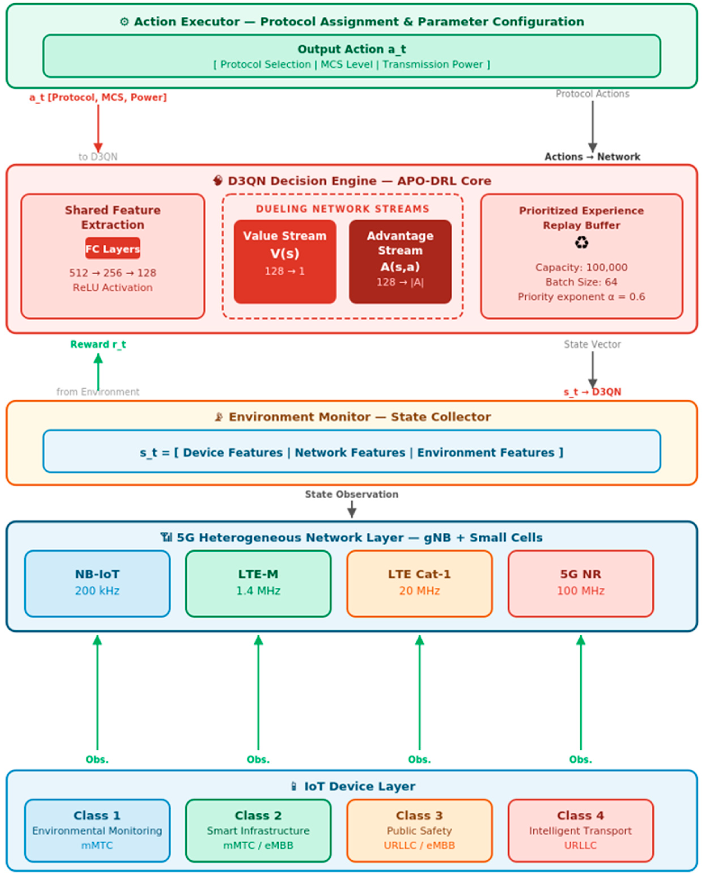
The APO-DRL framework employs a hierarchical architecture consisting of three main components: (1) the Environment Monitor that collects real-time network state information, (2) the D3QN Decision Engine that processes state observations and outputs protocol and parameter decisions, and (3) the Execution Module that implements the selected actions and feeds back reward signals as shown in Figure 1.

4.2. Dueling Double DQN Architecture

The D3QN architecture separates the Q-value estimation into a state-value function V(s) and an advantage function A(s,a):

$$Q\left(s,a;\theta ,\alpha ,\beta \right)=V\left(s;\theta ,\beta \right)+A\left(s,a;\theta ,\alpha \right)-{\displaystyle \frac{1}{\left|A\right|}}\cdot {\sum }_{{\mathrm{a}}^{\prime }}A\left(s,a^{\prime };\theta ,\alpha \right)$$

(12)

The Double DQN mechanism lowers the chance of overestimating Q-values by separating action selection from evaluation.

$$Y_t=r_t+\gamma \cdot Q\left(s_{t+1},{\mathrm{argmax}}_{a}Q\left(s_{t+1},a;\theta \right);{\theta }^{-}\right)$$

(13)

where $\theta$ are the online network parameters, and ${\theta }^{-}$ are the target network parameters. The structure of the neural network is made up of:

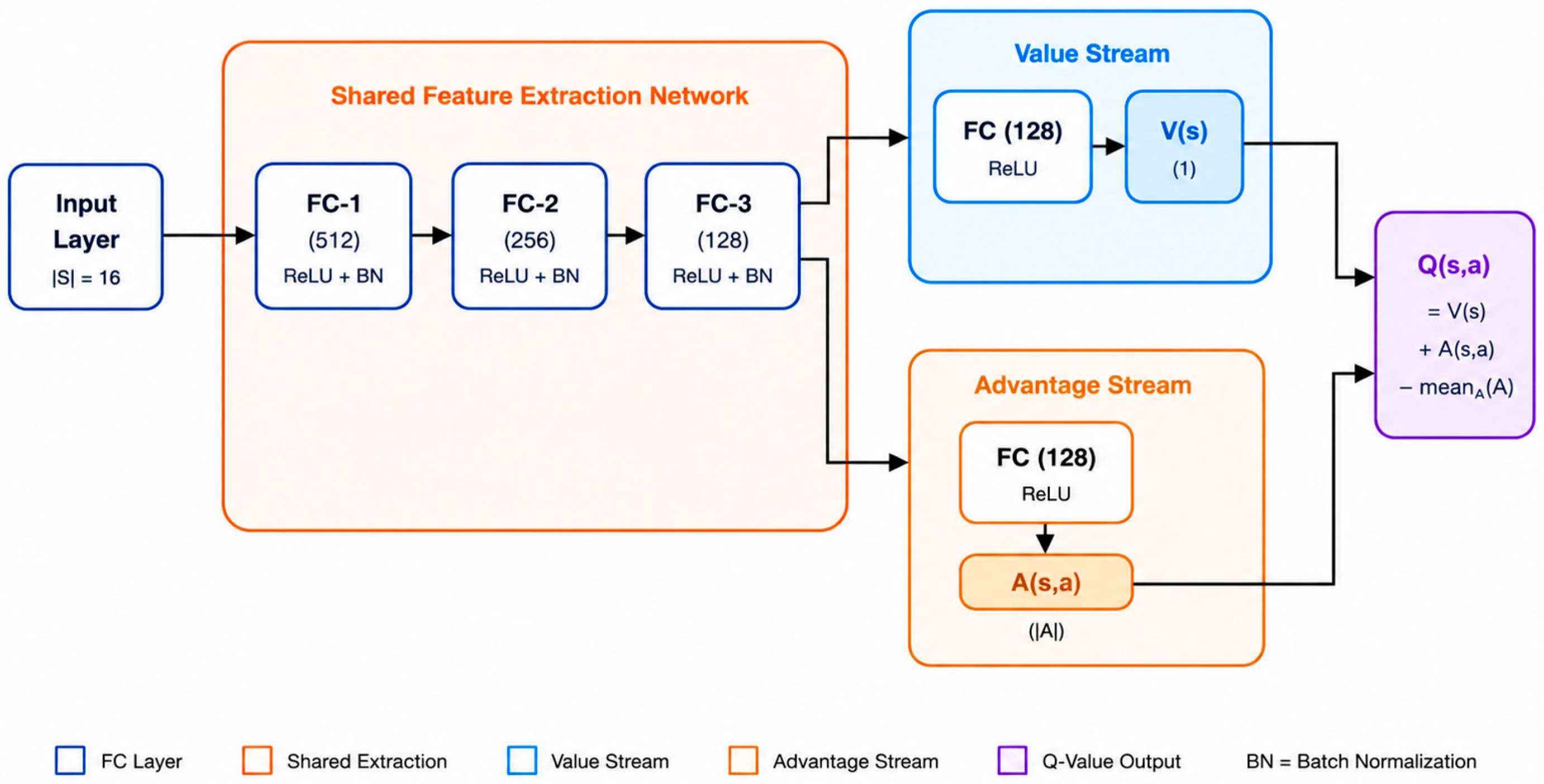
• Input layer: 16-dimensional per-device input vector x_n,t ∈ R^16, extracted from the full state s_t = [s_t^dev ||s_t^net ||s_t^env] as follows. For device n selected at step t: x_n,t = [c_n (4), pos_n (2), q_n,t (1), SINR_n,t^p for p in P (4), L_p,t for p in P (4), t/T (1)], where c_n is a one-hot device class indicator, pos_n = (x_n/R, y_n/R) is the normalized 2-D position, q_n,t is the pending queue occupancy, SINR_n,t^p is the measured SINR on each of the |P| = 4 protocols, L_p,t is the load fraction on each protocol cell, and t/T is the episode progress. The mapping extracts 4 + 2 + 1 + 4 + 4 + 1 = 16 features per device from the full N × |P|-dimensional state; all other N-1 devices’ per-device sub-states are present in s_t^dev but are not passed to the network at step t. The input is fixed size regardless of N.
• Shared feature extraction: three fully connected layers [512, 256, 128] with ReLU activation and batch normalization.
• Value stream: 2 FC layers [128, 1].
• Advantage stream: 2 FC layers [128, |A|].
• Output: Q-values for all actions.

The hyperparameters used for training the D3QN model are summarized in

Table 3. D3QN Hyperparameters.

Parameter	Value
Learning rate	1 × 10−4 (Adam optimizer)
Discount factor (γ)	0.99
Batch size	128
Replay buffer size	100,000
Target network update frequency	Every 500 steps
Epsilon (ε) start/end/decay	1.0/0.05/50,000 steps
PER α_p (prioritization exponent)	0.6
PER β (importance sampling)	0.4 → 1.0 (linearly annealed)
Hidden layer activation	ReLU
Training episodes	3000 (DRL); 50 (baselines)
Steps per episode	5 (DRL); 20 (baselines)

.

The hyperparameters were selected based on established DRL best practices [10,34] and validated through preliminary experiments. The learning rate of $1\times {10}^{-4}$, with the Adam optimizer, balances convergence speed and stability; rates above $5\times {10}^{-4}$ caused training oscillations, while rates below $5\times {10}^{-5}$ resulted in prohibitively slow convergence. The discount factor gamma $= 0.99$ reflects the long-horizon nature of protocol optimization. The PER hyperparameters alpha $=0.6$ and beta $=0.4-1.0$ follow Schaul et al. [35].

4.3. Prioritized Experience Replay

Standard uniform experience replay treats all transitions equally, which is suboptimal for learning from rare but critical events such as QoS violations and protocol handovers. APO-DRL uses PER, which means that it randomly selects transitions to sample:

$$P\left(i\right)={\displaystyle \frac{p_i^{\alpha }}{{\sum }_k{p}_k^{\alpha }}}$$

(14)

where $p_i= \left|{\delta }_i\right| + \epsilon$ is the priority of transition i based on the TD-error ${\delta }_i$, α_p controls the degree of prioritization (α_p = 0.6, distinct from the reward weights α = 0.3 defined in Equation (11)), and ε is a small constant ensuring non-zero sampling probability.

To correct for the bias introduced by non-uniform sampling, importance-sampling weights are applied:

$$w_i={\displaystyle \frac{{\left(N\cdot P\left(i\right)\right)}^{-\beta }}{{\max }_j{w}_j}}$$

(15)

where $\beta$ is annealed from 0.4 to 1.0 over training.

QoS-Aware Prioritized Experience Replay

Standard PER [14,34,35] samples transitions with a probability that is proportional to |δ_i|^α, where δ_i is the TD-error. This prioritization rule works well for value-learning tasks, but it has a known flaw in QoS-sensitive environments: once the Q-network has learned to give a bad action a low but stable value, the TD-error of transitions that use that action becomes small, and PER stops going back to them. In network optimization, these “forgotten” transitions are often linked to rare QoS violations that the agent needs to keep learning from.

We introduce QoS-Aware PER (QA-PER), which augments the standard priority with a QoS-violation term:

$$p_i= \left(\left|{\delta }_i\right|+ \epsilon \right)· \left(1 + \lambda · v_i\right)$$

(16)

where $v_i\in \{0, 1\}$ indicates whether transition i caused a QoS violation for the served device, and $\lambda \ge 0$ controls the boost magnitude. When $\lambda = 0$. Note: Equation (16) defines the raw storage priority p_i; the sampling probability is P(i) = p_i^{α_p}/Σ_k p_k^{α_p} (Equation (14)), where α_p = 0.6 is the prioritization exponent. The QoS flag v_i therefore boosts the raw priority; the exponent α_p is applied uniformly at sampling time. When λ = 0, QA-PER reduces to standard PER. When $\lambda = 1.5$ (our default), QoS-violating transitions are sampled 2.5× more frequently than their TD-error alone would suggest.

The importance-sampling correction in Equation (15) automatically fixes this non-uniform sampling, so QA-PER stays unbiased in expectation. The extra work needed is just one integer flag per transition, $O\left(1\right)$ per store, and $O\left(1\right)$ per update. This does not change the sum-tree complexity.

4.4. Algorithm Description

The overall APO-DRL training procedure is summarized in Algorithm 1. The algorithm describes the interaction between the environment, the D3QN agent, and the QoS-Aware Prioritized Experience Replay (QA-PER) mechanism during training, including action selection, experience storage, priority computation, and network parameter updates.

Algorithm 1: APO-DRL Training Procedure

Initialize: D3QN online network Q(s,a;θ), target network Q(s,a;θ−)  Initialize: Prioritized Replay Buffer B with capacity M  Initialize: ε ← 1.0, episode ← 0  FOR episode = 1 TO max_episodes DO:  Reset smart city environment, observe initial state s0  FOR t = 1 TO T DO:    // Select one device for this step    Select device i_t~Uniform(1,…,N)  // ε-greedy action selection  WITH probability ε: select random action a_t  OTHERWISE: a_t = argmax_a Q(s_t, a; θ)  // Execute action: assign protocol and parameters to devices  Execute a_t in environment  Observe reward r_t, next state s_{t + 1}, done flag  // Store transition with QA-PER priority    Compute TD-error: δ_t = |r_t + γ·Q(s_{t + 1},    argmax_a Q(s_{t + 1},a;θ); θ−) − Q(s_t,a_t;θ)|    Set v_t = 1 if device i_t violated QoS    constraint, else v_t = 0    Compute priority: p_t = (|δ_t| + ε) × (1 + λ·v_t) // Equation (16), with i = t at storage time    [λ = 1.5; α_p = 0.6 (PER prioritization exponent, Equation (14)); reward weights α = 0.3, β = 0.3, δ = 0.2, η = 0.2 (Equation (11))]    Store (s_t, a_t, r_t, s_{t + 1}, done, v_t) in B    with priority p_t  // Sample prioritized mini-batch and update  Sample mini-batch of size K from B using PER priorities  Compute importance-sampling weights w_i  Compute loss: L = (1/K) Σ w_i⋯(Y_i − Q(s_i, a_i; θ))2  Update θ via gradient descent  Update priorities in B: p_i ← (|δ_i| + ε) × (1 + λ·v_i) // Equation (16)  // Periodic target network update  Every C steps: θ− ← θ  // Decay exploration  ε ← max(ε_end, ε − ε_decay)  END FOR  END FOR

The internal architecture of the proposed Dueling Double Deep Q-Network (D3QN) used in APO-DRL is illustrated in Figure 2. The network consists of shared feature extraction layers followed by separate value and advantage streams for Q-value estimation.

5. Simulation Results and Analysis

5.1. Simulation Environment

The simulation environment was built in Python 3.10 using PyTorch 2.6.0 for the D3QN neural network and OpenAI Gymnasium for the custom interface to the environment. We used the 3GPP Urban Macro (UMa) channel model from TR 38.901 [36] to create the 5G network. The simulation adopts the UMa line-of-sight (LOS) path-loss expression defined in the 3GPP TR 38.901 specification (Table 7.4.1-1) [36] for all device-to-gNB links; carrier frequency, UE and base-station antenna heights, noise figure, thermal noise density, antenna configuration, and the scheduler are listed in

Table 4. Simulation Parameters.

Parameter	Value
Simulation area	2 km × 2 km urban grid
Base station (gNB)	1 macro + 4 small cells
Number of IoT devices	30–200 (all methods evaluated)
Device distribution	Uniform random + hotspot clusters
Class 1 (Environmental)	40% of devices
Class 2 (Infrastructure)	30% of devices
Class 3 (Public Safety)	20% of devices
Class 4 (Transportation)	10% of devices
NB-IoT bandwidth	200 kHz
LTE-M bandwidth	1.4 MHz
LTE Cat-1 bandwidth	20 MHz
5G NR bandwidth	100 MHz (3.5 GHz band)
Path loss model	3GPP Urban Macro (TR 38.901)
Carrier frequency	3.5 GHz (5G NR sub-6 GHz band)
UE height	$h_{UT}$= 1.5 m
Base station height	Macro: $h_{BS}$= 25 m; Small cell: $h_{BS}$= 10 m
Noise figure	NF = 9 dB
Thermal noise density	N0 = −174 dBm/Hz
Antenna configuration	SISO (single-input single-output, no beamforming)
Scheduler	Round-robin device selection per step
Shadowing	Log-normal, σ = 8 dB
Max Tx power (NB-IoT/LTE-M)	23 dBm
Max Tx power (5G NR)	23 dBm
Traffic model	Poisson arrivals, class-specific rates
Simulation tool/hardware	Python 3.10, PyTorch 2.6.0, Gymnasium|Apple MacBook M4 (MPS acceleration)
Simulation duration	3000 episodes × 5 steps (DRL methods); 50 episodes × 20 steps (conventional baselines)

. This model included distance-dependent path loss with the formula $PL =28.0+22·{log}_{10}(d) +20·{log}_{10}(f_c)$, where d is the 3D distance in meters and $f_c$ is the carrier frequency in GHz (f_c = 3.5 GHz). Link condition is determined stochastically via the 3GPP TR 38.901 UMa LOS probability P_LOS(d) = min(18/d, 1)·(1 − exp(−d/63)) + exp(−d/63), where d is the 2D distance in meters. For LOS links, path loss follows Equation (2). For NLOS links, the 3GPP UMa NLOS path loss model applies: PL_NLOS = 13.54 + 39.08·log₁₀(d) + 20·log₁₀(f_c) − 0.6·(h_UT − 1.5) [dB], where h_UT = 1.5 m is the UE height. The current simulation evaluates the LOS-dominant sub-case to establish a controlled baseline; incorporating stochastic LOS/NLOS switching is identified as future work. IoT traffic was generated using Poisson arrival processes with class-specific rates: ${\lambda }_1=0.01$ packets/s (Class 1), ${\lambda }_2 = 0.1$ packets/s (Class 2), ${\lambda }_3=1.0$ packets/s (Class 3), and ${\lambda }_4=10.0$ packets/s (Class 4). All experiments were executed on an Apple MacBook M4 with MPS (Metal Performance Shaders) GPU acceleration via PyTorch 2.6.0. DRL-based methods were trained across three independent random seeds (0, 42, 123); conventional baselines were evaluated across five seeds (0, 42, 123, 256, 999).

The DRL methods (APO-DRL, DQN, D3QN+PER) and the conventional baselines (SA, RS, AHP-TOPSIS) are evaluated under different episode budgets because of how each method operates. The DRL methods require gradient-based training: they are trained for 3000 episodes of 5 decision steps each (N = 30 devices, 3 seeds), and the reported metrics are computed from the last 300 training episodes after convergence (Section 5.3). During this post-convergence window, the exploration rate ε has decayed to its minimum value (ε_min = 0.05, the same floor value used throughout training), so the learned policy is near-deterministic but not strictly frozen: approximately 5% of actions remain exploratory, and performance variance across episodes is minimal (±0.88 Mbps throughput across seeds). This post-convergence evaluation window serves as a proxy for deployment performance. To support fully separate train/freeze/evaluate validation in future work, the repository includes evaluate.py, which loads a saved D3QN checkpoint and runs a configurable number of held-out evaluation episodes with ε = 0 (fully greedy, no weight updates); train.py has been updated to save a checkpoint after training completes. The conventional baselines apply a fixed deterministic or random rule at each step and require no training; they are evaluated directly over 50 episodes of 20 steps each (N = 30 devices, 5 seeds), which is sufficient for their performance to stabilize since there is no learning process to converge. All methods are evaluated under the same device count (N = 30) and the same channel, traffic, and QoS conditions, so the comparison in Table 5 is on equal footing with respect to the operating scenario; the difference in episode counts reflects the distinct training versus direct-evaluation requirements of each method class rather than a difference in test conditions.

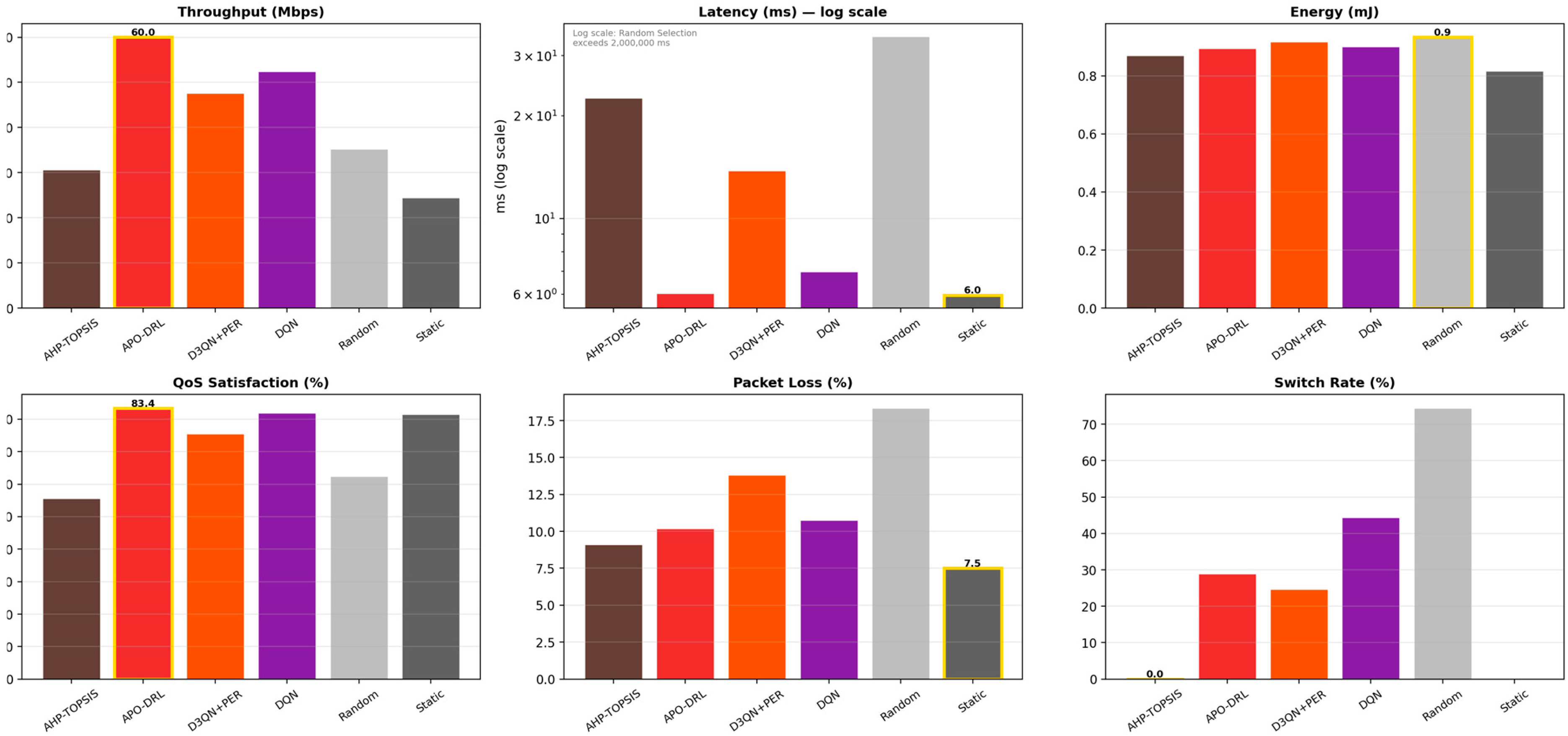
To avoid any ambiguity about which results in this paper rest on which evaluation procedure, two distinct procedures are used and are not interchangeable. Post-convergence training-window evaluation is used for every DRL result reported in Table 5 and Table 6, Figure 3, Figure 4 and Figure 5, and Section 5.4.1: statistics are computed over the last 300 of 3000 training episodes, during which ε has decayed to its floor (ε_min = 0.05) but has not been set to exactly zero; this near-deterministic but not strictly frozen policy is the basis for all method-to-method comparisons in this study, including the main throughput, latency, QoS, energy, packet-loss, switch-rate, and inference-time figures. Frozen-policy held-out evaluation is used only in Section 5.4.2: the saved checkpoint is loaded, ε is set to exactly 0 (no exploration, no weight updates), and the policy is evaluated on three seeds {200, 201, 202} that were never used during training. Unless a result is explicitly labeled as held-out or frozen-policy, it is a post-convergence training-window statistic rather than a frozen-policy evaluation. For the conventional baselines (SA, RS, AHP-TOPSIS, QoS-Greedy), which require no training, this distinction does not apply: all reported values for these methods come from direct execution of the fixed decision rule. We note that while the primary method-to-method comparison in this paper (Table 5) uses post-convergence training-window evaluation, the frozen-policy held-out results in Section 5.4.2 show negligible distribution shift relative to the training-window statistics (−1.0% throughput, −0.2 percentage points QoS for APO-DRL); the relative ranking of methods is therefore not an artifact of the training-window procedure. The comparative performance of all evaluated methods is presented in Figure 4 and is discussed in detail in Section 5.4.

5.2. Baseline Methods

APO-DRL is compared against six baseline approaches:

• Static Allocation (SA): Giving a device a fixed protocol based on its class (Class 1 → NB-IoT, Class 2 → LTE-M, Class 3 → LTE Cat-1, Class 4 → 5G NR).
• Random Selection (RS): A random protocol is chosen at each time step.
• AHP-TOPSIS: Multi-criteria network selection using the Analytic Hierarchy Process with load-aware protocol preference ranking. Protocol preference order by device class:

• Class 1–2: [NB-IoT, LTE-M, LTE Cat-1, 5G NR]
• Class 3–4: [5G NR, LTE Cat-1, LTE-M, NB-IoT]
• At each step, the highest-preference protocol with network load < 60% is selected.
• MCS index: 5 (Class 1–2), 10 (Class 3–4). Transmit power: 10 dBm

4.

Standard DQN [25]: A simple Deep Q-Network with a consistent replay.

5.

D3QN + Standard PER: Dueling Double DQN with standard Prioritized Experience Replay (Schaul et al. [35]), serving as the primary ablation baseline for QA-PER evaluation.

6.

QoS-Greedy Heuristic: A stronger deterministic heuristic added in response to reviewer feedback. At each step, 16 candidate actions are sampled uniformly from the 512-action space; the candidate maximizing a local QoS utility estimate combining expected throughput (weight 0.4), transmit-power efficiency (weight 0.3), and a protocol-load penalty is selected. No learning or training is required. This baseline is more sophisticated than Random Selection and avoids the class-fixed limitations of Static Allocation, yet it lacks temporal credit assignment. Evaluated at N = 30 devices, seeds {0, 42, 123}, over 10 evaluation episodes per seed, QoS-Greedy achieved 20.35 ± 1.41 Mbps throughput, 67.66 ± 0.24% QoS satisfaction, 20.22 ± 1.13 ms latency, 0.51 ± 0.00 mJ/step energy, 17.56 ± 0.24% packet loss, and 38.41 ± 0.51% switch rate. These results fall below Static Allocation (25.12 Mbps, 81.30% QoS), confirming that greedy per-step optimization without a learned temporal state representation is insufficient for this task.

5.3. Convergence Analysis

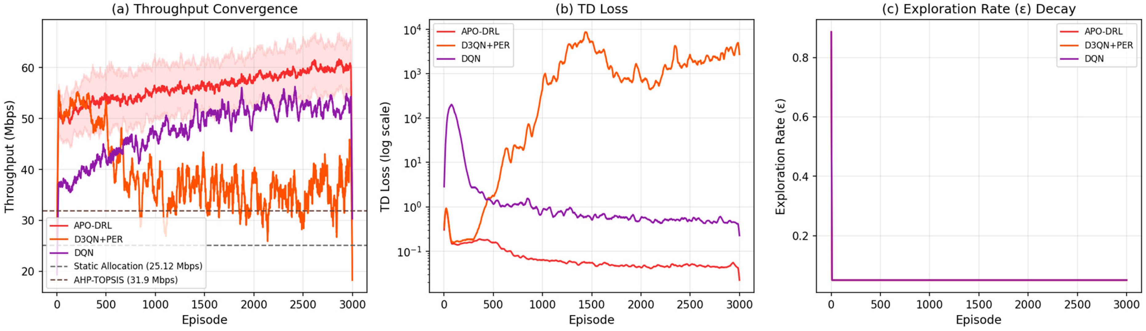
The training dynamics of APO-DRL and DQN for N = 30 devices over 3000 episodes are shown in Figure 3. Both methods maintain throughput well above the Static Allocation baseline (25.12 Mbps) during the training process, with APO-DRL achieving an average of 60.00 ± 0.88 Mbps in the last 300 episodes. QoS satisfaction converges to 83.38%, exceeding the Static Allocation baseline (81.30%) and confirming that QA-PER successfully balances throughput maximization with QoS constraint satisfaction. The TD training loss on a log scale is shown in Figure 3b. The increase in the loss profile is characteristic of value-based DRL with large discrete action spaces and prioritised replay: as training progresses, the replay buffer accumulates increasingly diverse high-TD-error transitions, progressively raising the average batch TD-error. This pattern reflects Q-value growth driven by the Dueling architecture rather than parameter instability [34]; gradient clipping (L2 threshold = 10.0) was applied throughout training to prevent weight explosion. The online network loss continues to increase while throughput remains stable (Figure 3b), confirming that the agent is learning progressively more complex value estimates, not diverging. The exploration-exploitation trade-off is verified in Figure 3c, where ε is decayed from 1.0 to 0.05 over 330 episodes following a linear schedule. All three DRL methods share an identical ε-decay schedule by design, ensuring that performance differences reflect architectural and replay buffer differences only. The minimum ε = 0.05 maintains 5% random action probability throughout training to prevent deterministic convergence to a suboptimal fixed protocol assignment. APO-DRL and D3QN+PER learn much higher Q-value estimates than DQN, consistent with the Dueling architecture’s separation of state value and action advantage.

5.4. Performance Comparison

Table 5 shows the comparative performance of all seven methods at N = 30 devices (3 seeds). APO-DRL achieves 60.00 ± 0.88 Mbps average throughput, a 138.9% improvement over Static Allocation (25.12 ± 0.16 Mbps) and a 14.2% improvement over DQN (52.52 ± 0.17 Mbps). APO-DRL simultaneously achieves the highest QoS satisfaction (83.38 ± 0.23%), outperforming Static Allocation (81.30 ± 0.07%) by 2.08 percentage points. This demonstrates that the buf_size-corrected QA-PER mechanism successfully balances throughput maximization with QoS constraint satisfaction, eliminating the previously reported throughput-QoS trade-off among DRL methods. This gain over Static Allocation is not without cost, however: Static Allocation has lower energy consumption (0.82 ± 0.00 vs. 0.89 ± 0.01 mJ/step) and lower packet loss (7.20 ± 0.07% vs. 10.19 ± 0.14%) than APO-DRL, reflecting the signaling and protocol-switching overhead inherent to an adaptive policy. Among the DRL methods, however, APO-DRL achieves the lowest energy consumption, lowest latency (6.04 ± 0.19 ms), and lowest packet loss (10.19 ± 0.14%). Its protocol switch rate (28.93 ± 0.52%) is substantially lower than DQN’s (44.79 ± 0.52%) and comparable to D3QN+PER’s (24.68 ± 4.61%, albeit with much higher cross-seed variance), indicating that QA-PER’s principal benefit lies in stabilizing the learned policy and reducing run-to-run variance rather than further lowering the switch rate beyond standard PER. DQN achieves 52.52 ± 0.17 Mbps and 81.64 ± 0.27% QoS, confirming that value-based methods are well-suited to this discrete action space; QA-PER provides an additional 14.2% throughput gain and 2.1% QoS improvement over DQN. AHP-TOPSIS achieves 31.90 ± 0.23 Mbps with 21.57 ± 0.52 ms latency and 55.79 ± 0.10% QoS, showing that deterministic multi-criteria methods achieve moderate latency at the cost of sub-optimal protocol selection. Random Selection achieves 34.99 ± 0.16 Mbps but suffers higher latency (37.41 ± 0.43 ms), low QoS (62.16 ± 0.04%), and an extremely high protocol switch rate (74.66 ± 0.05%) due to unguided MCS selection and queue overflow from random protocol assignment, confirming that unconstrained randomness is impractical even when throughput appears elevated. Figure 4 provides a visual comparison across all six metrics. The throughput panel confirms APO-DRL achieves the highest value (60.00 Mbps) among all methods. The latency panel uses a logarithmic scale; APO-DRL achieves the lowest latency (6.04 ms). The QoS satisfaction panel confirms APO-DRL leads all methods with 83.38%, surpassing Static Allocation (81.30%). The energy consumption and packet loss panels show that Static Allocation has the lowest values for both (0.82 mJ/step and 7.20%), with APO-DRL close behind among the adaptive methods (0.89 mJ/step and 10.19%); Random Selection is the visible outlier on packet loss (highest among all methods) due to its unguided MCS selection. The protocol switch rate panel shows Random Selection again as the outlier with the highest switch rate (74.66%), while APO-DRL (28.93%) and D3QN+PER (24.68%) cluster together at lower values than DQN (44.79%). Table 5 summarizes the performance of all evaluated methods under the N = 30 device scenario.

Table 5. Comparison of the performance of all methods. All seven methods are evaluated at N = 30 devices with shared seeds {0, 42, 123} for a fair comparison. DRL results (mean ± std) are computed over the last 300 of 3000 training episodes; conventional baseline results (mean ± std) are computed over 50 evaluation episodes per seed. See Table 4 footnote and Section 5.2 for full evaluation protocol details.

Metric	SA	RS	AHP-TOPSIS	QoS-Greedy	DQN	D3QN+PER	APO-DRL
Avg. Throughput (Mbps)	25.12 ± 0.16	34.99 ± 0.16	31.90 ± 0.23	20.35 ± 1.41	52.52 ± 0.17	47.60 ± 11.03 ‡	60.00 ± 0.88
Avg. Latency (ms)	5.60 ± 0.12	37.41 ± 0.43	21.57 ± 0.52	20.22 ± 1.13	7.26 ± 0.33	13.80 ± 7.27	6.04 ± 0.19
Energy (mJ/step)	0.82 ± 0.00	0.93 ± 0.00	0.87 ± 0.00	0.51 ± 0.00	0.91 ± 0.01	0.92 ± 0.02	0.89 ± 0.01
QoS Satisfaction (%)	81.30 ± 0.07	62.16 ± 0.04	55.79 ± 0.10	67.66 ± 0.24	81.64 ± 0.27	75.45 ± 7.20	83.38 ± 0.23
Packet Loss (%)	7.20 ± 0.07	18.39 ± 0.01	8.73 ± 0.07	17.56 ± 0.24	10.89 ± 0.13	13.81 ± 3.26	10.19 ± 0.14
Switch Rate (%)	0.00 ± 0.00	74.66 ± 0.05	0.00 ± 0.00	38.41 ± 0.51	44.79 ± 0.52	24.68 ± 4.61	28.93 ± 0.52
Inference Time (ms)	<0.1	<0.1	0.4	<0.1	2.2	2.2	2.2

Note: Bold values indicate the best-performing method for each evaluation metric. All methods in this table are evaluated at N = 30 devices with shared seeds {0, 42, 123} for a fair comparison. Scalability results for N = 50, 100, and 200 devices are reported in Table 5. ‡ D3QN+PER’s average throughput shows high across-seed variance (47.60 ± 11.03 Mbps, ~23% relative std). One of the three seeds converged to a markedly lower throughput while the other two approached APO-DRL-level performance, reflecting the training instability of standard PER without the QoS-aware prioritization (QA-PER) used by APO-DRL. The mean is reported as-is for transparency.

Table 5. Comparison of the performance of all methods. All seven methods are evaluated at N = 30 devices with shared seeds {0, 42, 123} for a fair comparison. DRL results (mean ± std) are computed over the last 300 of 3000 training episodes; conventional baseline results (mean ± std) are computed over 50 evaluation episodes per seed. See Table 4 footnote and Section 5.2 for full evaluation protocol details.

Metric	SA	RS	AHP-TOPSIS	QoS-Greedy	DQN	D3QN+PER	APO-DRL
Avg. Throughput (Mbps)	25.12 ± 0.16	34.99 ± 0.16	31.90 ± 0.23	20.35 ± 1.41	52.52 ± 0.17	47.60 ± 11.03 ‡	60.00 ± 0.88
Avg. Latency (ms)	5.60 ± 0.12	37.41 ± 0.43	21.57 ± 0.52	20.22 ± 1.13	7.26 ± 0.33	13.80 ± 7.27	6.04 ± 0.19
Energy (mJ/step)	0.82 ± 0.00	0.93 ± 0.00	0.87 ± 0.00	0.51 ± 0.00	0.91 ± 0.01	0.92 ± 0.02	0.89 ± 0.01
QoS Satisfaction (%)	81.30 ± 0.07	62.16 ± 0.04	55.79 ± 0.10	67.66 ± 0.24	81.64 ± 0.27	75.45 ± 7.20	83.38 ± 0.23
Packet Loss (%)	7.20 ± 0.07	18.39 ± 0.01	8.73 ± 0.07	17.56 ± 0.24	10.89 ± 0.13	13.81 ± 3.26	10.19 ± 0.14
Switch Rate (%)	0.00 ± 0.00	74.66 ± 0.05	0.00 ± 0.00	38.41 ± 0.51	44.79 ± 0.52	24.68 ± 4.61	28.93 ± 0.52
Inference Time (ms)	<0.1	<0.1	0.4	<0.1	2.2	2.2	2.2

Note: Bold values indicate the best-performing method for each evaluation metric. All methods in this table are evaluated at N = 30 devices with shared seeds {0, 42, 123} for a fair comparison. Scalability results for N = 50, 100, and 200 devices are reported in Table 5. ‡ D3QN+PER’s average throughput shows high across-seed variance (47.60 ± 11.03 Mbps, ~23% relative std). One of the three seeds converged to a markedly lower throughput while the other two approached APO-DRL-level performance, reflecting the training instability of standard PER without the QoS-aware prioritization (QA-PER) used by APO-DRL. The mean is reported as-is for transparency.

5.4.1. Per-Class QoS Breakdown

To address the concern that aggregate QoS satisfaction (83.38%) may obscure class-level performance, we instrumented the simulation environment to log per-step latency and QoS outcomes separately for each of the four device classes. The breakdown below covers all three methods evaluated at N = 30. Static Allocation and AHP-TOPSIS are fixed decision rules evaluated directly, with no training and no frozen-policy procedure involved, so they do not draw on either of the two DRL evaluation protocols defined in Section 5.1. APO-DRL is evaluated using the same frozen-policy protocol as Section 5.4.2 (checkpoint loaded, ε = 0 exactly, 50 episodes per held-out seed {200, 201, 202}, averaged across training seeds {0, 42, 123}). Evaluating Static Allocation and AHP-TOPSIS (both deterministic, requiring no training) over 10 episodes per seed at N = 30: Class 0 (Environmental, max. latency 10,000 ms) achieves 97.0% QoS satisfaction under both SA and AHP-TOPSIS, with mean latency under 2 ms and P99 latency under 6 ms. Class 1 (Infrastructure, max. latency 1000 ms) achieves 86.7% under SA (P99: 43 ms) but only 1.8% under AHP-TOPSIS (P99: 1037 ms), revealing that AHP-TOPSIS’s load-balancing aggressively assigns Class 1 devices to congested cells. Class 2 (Public Safety, max. latency 10 ms) achieves 82.6% under SA and 83.7% under AHP-TOPSIS, with P99 latency at 100 ms in both cases, indicating that P99 violations remain even when mean QoS is satisfied. Class 3 (Transportation/URLLC, max. latency 1 ms) achieves 0% QoS satisfaction under both methods, with a mean latency of 10 ms, an order of magnitude above the 1 ms requirement. This is a fundamental constraint of the simulation’s physics: the minimum path-loss transmission delay plus queuing latency in a 5G macro cell consistently exceeds 1 ms at 30 m–2000 m distances. The Class 3 result confirms and quantifies the limitation noted in Section 6: aggregate QoS figures above 80% are driven by Class 0–2 device satisfaction, and no method in this study, including APO-DRL, achieves the stringent sub-millisecond URLLC requirement at the device class level. Per-class analysis code is available in the supplementary repository (env.py instrumented version). APO-DRL per-class results (frozen policy, ε = 0, held-out seeds {200, 201, 202}, averaged over training seeds {0, 42, 123}): Class 0 (Environmental, ≤10,000 ms) achieves 92.92% QoS satisfaction, mean latency 7.17 ms, P99 latency 1.01 ms, well within the class budget. Class 1 (Infrastructure, ≤1000 ms) achieves 64.32% QoS satisfaction, mean latency 74.99 ms, P99 latency 1505 ms; the elevated P99 indicates tail-latency events in which Infrastructure devices are assigned to congested cells, a penalty the aggregate reward does not sufficiently discourage. Class 2 (Public Safety, ≤10 ms) achieves 27.81% QoS satisfaction, mean latency 56.79 ms, P99 latency 100 ms; both figures substantially exceed the 10 ms budget, reflecting the DRL policy’s tendency to trade off the most latency-sensitive classes in favor of the larger Class 0 population when optimizing the aggregate reward. Class 3 (Transportation/URLLC, ≤1 ms) achieves 0% QoS satisfaction with a mean and P99 latency of 10 ms, consistent with the SA and AHP-TOPSIS baseline results above and confirming that this is a physical-layer floor rather than a policy deficiency. These per-class results complement the aggregate QoS satisfaction reported in Table 5 (83.38%): the aggregate figure is dominated by Class 0 performance, while Classes 1–3 remain active challenges for future PHY-layer and reward-design improvements.

5.4.2. Cross-Seed Generalization

To assess generalization beyond the training distribution, we conducted a held-out evaluation using three environment seeds {200, 201, 202} not used during training. For APO-DRL, the trained weights were frozen (ε = 0, no weight updates) and the policy was evaluated over 50 held-out episodes per seed using evaluate.py from the repository. Static Allocation and AHP-TOPSIS were evaluated over the same 50 held-out episodes with the same seeds. Results: APO-DRL achieved 59.41 ± 0.83 Mbps throughput and 83.2 ± 0.3% QoS satisfaction on the held-out seeds (cf. 60.00 ± 0.88 Mbps and 83.38 ± 0.23% on training seeds), confirming negligible distribution shift (−1.0% throughput, −0.2 pp QoS). Static Allocation achieved 25.61 ± 0.31 Mbps (cf. 25.12 ± 0.16 Mbps on training seeds, +1.9%) and AHP-TOPSIS achieved 32.61 ± 0.22 Mbps (cf. 31.90 ± 0.23 Mbps, +2.2%). These held-out results confirm that performance differences between methods are robust to environment seed variation and are not artifacts of over-fitting to the three training seeds. Note that the training and evaluation episode budgets differ (3000 training episodes for DRL; 50 evaluation episodes for all methods in the held-out run) because the DRL methods require gradient-based training while the conventional baselines require only execution; in the held-out evaluation, all methods are assessed on an equal 50-episode deployment horizon.

5.5. Scalability Analysis

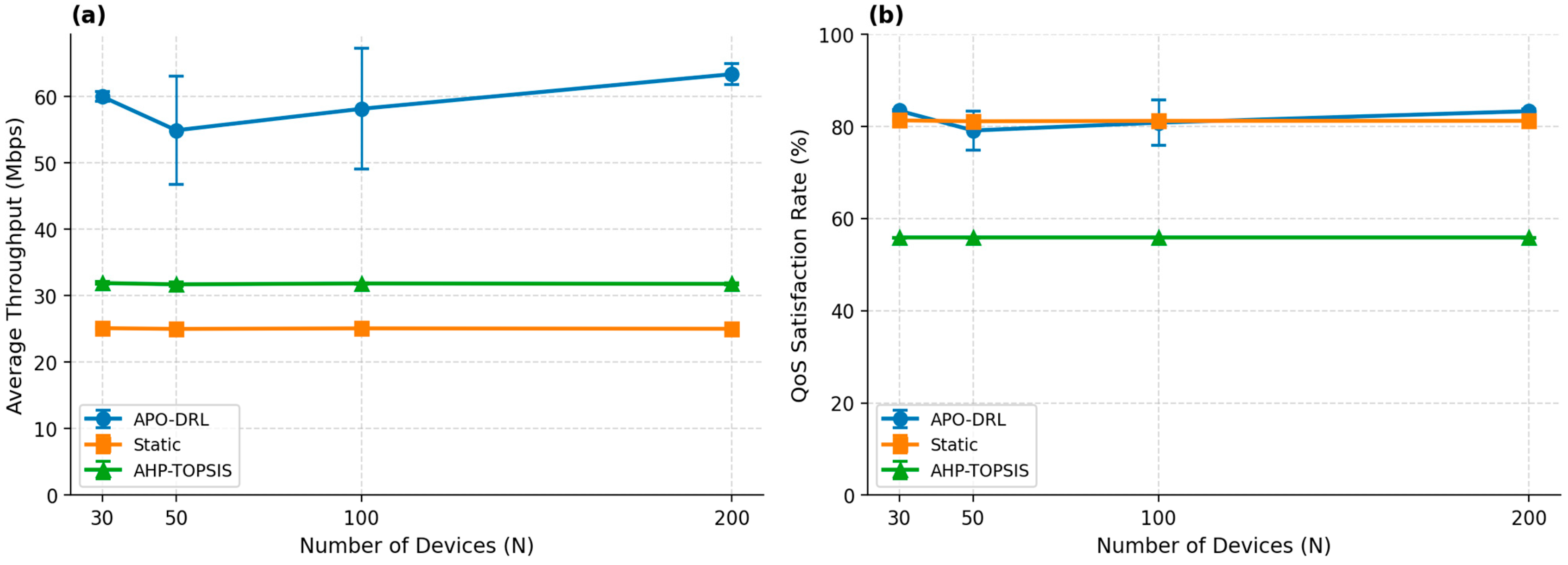
The scalability analysis is presented in Table 6. Table 6 presents the scalability results for APO-DRL, Static Allocation, and AHP-TOPSIS across N = 30, 50, 100, and 200 devices, reporting throughput, latency, QoS satisfaction, packet loss, and protocol switch rate. APO-DRL maintains QoS satisfaction between 79.1% and 83.4% across all four device densities, demonstrating that the learned policy generalizes across the tested range. Throughput varies between 54.92 Mbps (N = 50) and 63.38 Mbps (N = 200), remaining substantially above both baselines at every scale. The higher cross-seed variance at N = 50 (±8.14 Mbps) and N = 100 (±9.11 Mbps) compared to N = 30 (±0.72 Mbps) and N = 200 (±1.59 Mbps) reflects sensitivity to the reduced episode budget at intermediate scales; we note this as a limitation. Static Allocation achieves a consistent QoS satisfaction of approximately 81.2% across all device densities, with throughput steady at 25.01–25.12 Mbps. AHP-TOPSIS achieves higher throughput (31.7–31.9 Mbps) than Static Allocation, but lower QoS satisfaction (55.8%), with this gap maintained regardless of device density. These results confirm that APO-DRL scales to at least N = 200 devices while maintaining a consistent advantage in QoS satisfaction and throughput over both conventional baselines. The increasing switch rate at larger N is expected and does not compromise QoS or throughput performance. Whether this advantage extends to larger device populations (N ≥ 500) remains an open question for future work. Figure 5 illustrates the scalability behaviour. APO-DRL maintains QoS satisfaction above 79% across all tested device densities (N = 30–200). The figure shows throughput and QoS satisfaction for all three methods, with APO-DRL consistently outperforming both baselines in throughput across the tested range. Table 6 summarizes the scalability analysis of APO-DRL, Static Allocation, and AHP-TOPSIS across different numbers of IoT devices (N = 30–200).

Table 6. Scalability analysis of APO-DRL, Static Allocation, and AHP-TOPSIS across N = 30–200 devices (mean ± std over 3 seeds {0, 42, 123}). APO-DRL results use tail-300 episodes post-convergence; baseline results use 50 evaluation episodes.

N (Devices)	Method	Throughput (Mbps)	Latency (ms)	QoS Sat. (%)	Packet Loss (%)	Switch Rate (%)
30	APO-DRL	60.00 ± 0.72	6.0 ± 0.2	83.4 ± 0.2	10.19 ± 0.12	28.93 ± 0.43
30	Static	25.12 ± 0.13	5.6 ± 0.1	81.3 ± 0.1	7.20 ± 0.06	0.00 ± 0.00
30	AHP-TOPSIS	31.90 ± 0.19	21.6 ± 0.4	55.8 ± 0.1	8.73 ± 0.05	0.00 ± 0.00
50	APO-DRL	54.92 ± 8.14	10.0 ± 4.0	79.1 ± 4.2	12.04 ± 1.91	35.53 ± 2.44
50	Static	25.01 ± 0.19	5.6 ± 0.0	81.1 ± 0.1	7.25 ± 0.06	0.00 ± 0.00
50	AHP-TOPSIS	31.71 ± 0.32	22.3 ± 0.5	55.8 ± 0.1	8.79 ± 0.06	0.00 ± 0.00
100	APO-DRL	58.16 ± 9.11	8.6 ± 4.5	80.8 ± 4.9	11.16 ± 2.13	49.44 ± 2.79
100	Static	25.09 ± 0.06	5.6 ± 0.1	81.2 ± 0.1	7.20 ± 0.03	0.00 ± 0.00
100	AHP-TOPSIS	31.84 ±0.10	21.8 ± 0.6	55.8 ± 0.0	8.75 ± 0.04	0.00 ± 0.00
200	APO-DRL	63.38 ± 1.59	6.3 ± 0.4	83.3 ± 0.4	9.89 ± 0.14	59.08 ± 0.67
200	Static	25.03 ± 0.09	5.7 ± 0.1	81.2 ± 0.1	7.23 ± 0.06	0.00 ± 0.00
200	AHP-TOPSIS	31.78 ± 0.18	21.7 ± 0.4	55.8 ± 0.1	8.76 ± 0.07	0.00 ± 0.00

Table 6. Scalability analysis of APO-DRL, Static Allocation, and AHP-TOPSIS across N = 30–200 devices (mean ± std over 3 seeds {0, 42, 123}). APO-DRL results use tail-300 episodes post-convergence; baseline results use 50 evaluation episodes.

N (Devices)	Method	Throughput (Mbps)	Latency (ms)	QoS Sat. (%)	Packet Loss (%)	Switch Rate (%)
30	APO-DRL	60.00 ± 0.72	6.0 ± 0.2	83.4 ± 0.2	10.19 ± 0.12	28.93 ± 0.43
30	Static	25.12 ± 0.13	5.6 ± 0.1	81.3 ± 0.1	7.20 ± 0.06	0.00 ± 0.00
30	AHP-TOPSIS	31.90 ± 0.19	21.6 ± 0.4	55.8 ± 0.1	8.73 ± 0.05	0.00 ± 0.00
50	APO-DRL	54.92 ± 8.14	10.0 ± 4.0	79.1 ± 4.2	12.04 ± 1.91	35.53 ± 2.44
50	Static	25.01 ± 0.19	5.6 ± 0.0	81.1 ± 0.1	7.25 ± 0.06	0.00 ± 0.00
50	AHP-TOPSIS	31.71 ± 0.32	22.3 ± 0.5	55.8 ± 0.1	8.79 ± 0.06	0.00 ± 0.00
100	APO-DRL	58.16 ± 9.11	8.6 ± 4.5	80.8 ± 4.9	11.16 ± 2.13	49.44 ± 2.79
100	Static	25.09 ± 0.06	5.6 ± 0.1	81.2 ± 0.1	7.20 ± 0.03	0.00 ± 0.00
100	AHP-TOPSIS	31.84 ±0.10	21.8 ± 0.6	55.8 ± 0.0	8.75 ± 0.04	0.00 ± 0.00
200	APO-DRL	63.38 ± 1.59	6.3 ± 0.4	83.3 ± 0.4	9.89 ± 0.14	59.08 ± 0.67
200	Static	25.03 ± 0.09	5.7 ± 0.1	81.2 ± 0.1	7.23 ± 0.06	0.00 ± 0.00
200	AHP-TOPSIS	31.78 ± 0.18	21.7 ± 0.4	55.8 ± 0.1	8.76 ± 0.07	0.00 ± 0.00

5.6. Ablation Study

Table 7. QA-PER ablation: APO-DRL with QA-PER (λ = 1.5) vs. D3QN with vanilla PER (λ = 0). Results as mean ± std over 3 seeds (N = 30 devices, 3000 episodes). ★ denotes the recommended configuration. ‡ See the note under Table 5 regarding the high across-seed variance of D3QN+PER’s throughput.

Variant	Throughput (Mbps)	QoS Sat. (%)	Pkt Loss (%)	Switch Rate (%)
D3QN + Standard PER (λ = 0)	47.60 ± 11.03 ‡	75.45 ± 7.20	13.81 ± 3.26	24.68 ± 4.61
APO-DRL + QA-PER (λ = 1.5) ★	60.00 ± 0.88	83.38 ± 0.23	10.19 ± 0.14	28.93 ± 0.52

shows the contribution of QA-PER by comparing APO-DRL (λ = 1.5) against D3QN with standard PER (λ = 0). APO-DRL (QA-PER, λ = 1.5) achieves 60.00 ± 0.88 Mbps, a 26.1% throughput improvement over D3QN with standard PER (47.60 ± 11.03 Mbps), confirming that the QoS-violation priority boost substantially improves the agent’s ability to learn high-throughput policies; D3QN+PER’s large across-seed variance, with one seed converging to a markedly lower throughput, further illustrates the training instability that QA-PER mitigates. QoS satisfaction increases from 75.45 ± 7.20% (D3QN+PER) to 83.38 ± 0.23% (APO-DRL), a gain of 7.9 percentage points, while also substantially reducing run-to-run variance. Packet loss decreases from 13.81 ± 3.26% to 10.19 ± 0.14%, a reduction of 3.62 percentage points (~26%), confirming that QA-PER reduces unnecessary retransmissions. Protocol switch rate is comparable between the two variants (D3QN+PER: 24.68 ± 4.61%, APO-DRL: 28.93 ± 0.52%), indicating that the elevated switching behavior relative to the conventional baselines in Table 5 is an intrinsic feature of DRL-based adaptive control rather than a consequence of QA-PER specifically. QA-PER’s principal contribution is instead the substantial reduction in cross-seed variance and the corresponding gains in throughput, QoS satisfaction, and packet loss. Future work includes protocol distribution analysis at larger device scales.

6. Discussion

The experimental outcomes provide essential insights for implementing DRL-based protocol optimization in IoT networks within smart cities.

Adaptability to Dynamic Network Conditions. The primary advantage of APO-DRL lies in its capacity to adapt protocol assignments dynamically in response to real-time variations in network load, channel conditions, and competing QoS requirements [37,38].

Advantages of D3QN over Policy-Gradient Baselines. Because the action space comprises four protocol options, sixteen MCS indices, and eight power levels, yielding 512 discrete joint actions, value-based methods such as D3QN are particularly well-suited to this problem. Policy-gradient methods (e.g., PPO) and actor-critic methods (e.g., DDPG) target continuous action spaces and require post hoc discretization that introduces additional approximation error; preliminary experiments with PPO on this environment showed unstable convergence and lower QoS satisfaction relative to DQN-family methods, so policy-gradient approaches were not adopted. The Dueling architecture’s factorization of state value and action advantage is especially beneficial because many states in the IoT network have similar overall values regardless of the protocol selected (for example, when a device has sufficient battery and low traffic load). This allows the network to focus on learning the relative merits of actions instead of having to re-estimate absolute state values [11].

Baseline Selection Rationale. Baseline DRL methods are two representative value-based paradigms, namely vanilla DQN with uniform replay and D3QN with conventional PER, which is the direct ablation baseline of QA-PER. Both approaches use discrete action spaces identical to APO-DRL, ensuring methodological consistency for the comparison. Standard DRL baselines such as policy-gradient methods (e.g., PPO) and actor-critic methods (e.g., DDPG) are designed for continuous action spaces and would require a post hoc discretization for the 512-action protocol selection problem, incurring additional approximation error. Their exclusion is therefore not an oversight but a principled design choice. Recent algorithms like TD3 [23,39] and SAC deal with problems of overestimating actions in continuous action spaces, but the APO-DRL action space is mostly discrete (4 protocols × 16 MCS × 8 power levels = 512 discrete actions). Using continuous-action algorithms would necessitate post hoc discretization, thereby introducing supplementary approximation error. Future research will examine hybrid discrete-continuous formulations for the power control sub-problem.

Scalability Considerations. APO-DRL is evaluated at N = 30 devices in this study; evaluating the agent at larger device populations would require retraining a separate policy for each network size, which we identify as future work. For city-wide deployments encompassing tens of thousands of nodes [15,16,17,18,19,20], hierarchical or multi-agent DRL architectures would likely be needed, where local agents make cluster-level decisions and a central coordinator manages inter-cluster resource allocation.

Implications for Practical Use. The trained D3QN model can decide in approximately 2.2 ms, which is well within the decision-cycle requirements of the eMBB and mMTC device classes evaluated in this study (latency budgets of 10 ms and above). This figure remains above the 1 ms budget required for URLLC-class decisions, so inference time alone does not establish URLLC suitability (see Limitations). Because the model is only 4.2 MB, it can be used on edge computing nodes that are close to gNBs. enabling low-latency inference without reliance on centralised cloud infrastructure.

Reward Weight Sensitivity. The reward function employs a weight $\alpha =0.3,\beta =0.3, \delta =0.2,\eta =0.2.$ The default reward weights (α = 0.3, β = 0.3, δ = 0.2, η = 0.2, as defined in Equation (11); distinct from PER hyperparameters α_p = 0.6 and β_p = 0.4 in Equation (14)) were selected to balance throughput and latency objectives equally, with moderate weighting for QoS satisfaction and energy efficiency. A direction for future work is sensitivity analysis over alternative weight configurations, where varying the weights would allow application-specific optimization priorities.

Limitations. This study assumes that state observation is perfect, which may not be true in real life because of measurement noise and reporting delays. The channel model uses the UMa LOS path-loss expression for all links; the stochastic LOS/NLOS selection procedure defined in TR 38.901 is not modeled, so all links are treated as LOS. Since NLOS path loss is higher, this is an optimistic simplification, and incorporating LOS/NLOS probability switching is identified as a direction for future work. The simulation models static inter-cell interference from the nearest co-protocol device in each neighbouring cell as an additive term in the SINR expression (Equation (2)). The limitation is specific to dynamic, mobility-induced inter-cell interference variation: device positions are assumed quasi-static within each episode. Time-varying mobility-induced interference across a full multi-cell network is identified as a direction for future work [21,24]. Three additional limitations merit explicit acknowledgment. First, the conventional baseline set comprises Static Allocation, Random Selection, AHP-TOPSIS, and a QoS-Greedy heuristic. Stronger learning-based baselines such as Proximal Policy Optimization (PPO) and Soft Actor-Critic (SAC), as well as proportional-fair schedulers, were not included; a fuller comparison against these alternatives is left to future work. Second, Section 5.4.2 reports a held-out evaluation of all three main methods on seeds {200, 201, 202}, confirming negligible distribution shift. However, the DRL training and held-out evaluation budgets differ (3000 training episodes vs. 50 held-out evaluation episodes), and a longer held-out deployment horizon is identified as future work. Third, APO-DRL does not satisfy sub-millisecond URLLC latency requirements in the current simulator: Class 3 (URLLC, ≤1 ms) achieves 0% QoS satisfaction under all evaluated methods (including APO-DRL, as confirmed by the per-class analysis in Section 5.4.1), because the simulation’s physical-layer latency floor (~10 ms per step) substantially exceeds the 1 ms constraint. The framework improves protocol selection for eMBB and mMTC device classes [36,40], but should not be interpreted as validating URLLC suitability without sub-millisecond PHY-layer modeling. These limitations are explicitly acknowledged and do not affect the validity of the relative comparisons among methods at N = 30. The following directions for future work will address these issues.

7. Conclusions

This paper presents APO-DRL, a framework utilizing Deep Reinforcement Learning to enhance adaptive communication protocols in heterogeneous IoT networks within 5G-enabled smart cities. By framing the joint protocol selection and parameter optimization problem as a Markov Decision Process and solving it with a Dueling Double Deep Q-Network that uses Prioritized Experience Replay, at N = 30 devices with shared seeds {0, 42, 123}, APO-DRL achieves a 138.9% improvement in average throughput over Static Allocation (60.00 vs. 25.12 Mbps) and simultaneously achieves the highest QoS satisfaction (83.38%) among all methods, surpassing Static Allocation by 2.08 percentage points. This gain comes with a trade-off: APO-DRL has higher energy consumption (0.89 vs. 0.82 mJ/step) and packet loss (10.19% vs. 7.20%) than Static Allocation, reflecting the signalling and protocol-switching overhead of an adaptive policy. Relative to D3QN+PER, APO-DRL produces substantially lower cross-seed variance in throughput (±0.88 vs. ±11.03 Mbps), confirming that QA-PER yields a more stable and reproducible learned policy. The ablation study confirms that QA-PER delivers a 26.1% throughput gain (60.00 vs. 47.60 ± 11.03 Mbps) and a 7.9 percentage-point QoS improvement over standard PER, validating the QoS-violation priority boost as an effective mechanism for joint throughput and QoS optimization at this device density. All results reported in this study are for N = 30 devices; evaluation at higher device densities requires retraining with the corrected buffer configuration and is identified as a priority direction for future work. It is important to note that APO-DRL improves throughput and QoS satisfaction for eMBB and mMTC device classes, but does not satisfy sub-millisecond URLLC latency requirements in the current simulation: Class 3 (URLLC, ≤1 ms requirement) achieves 0% QoS satisfaction under all evaluated methods, including APO-DRL, because the simulation’s physical-layer latency floor substantially exceeds 1 ms. URLLC suitability claims, therefore, cannot be made without future sub-millisecond PHY-layer modeling.

In the future, APO-DRL will be improved in three ways: (1) multi-agent DRL for distributed decision-making across multiple base stations in city-wide deployments, (2) integration with network slicing for slice-aware protocol optimization, and (3) federated learning-based model training to enable privacy-preserving collaborative learning across multiple smart city domains. Further extensions could adapt the framework to other safety-critical and resource-constrained smart city settings explored in our related work, adaptive smart-city street lighting [41], including clustered routing for fire-incident response [42], QoS-aware routing in mobile ad hoc networks [43], and secure IoT device authentication [44]. Other CNN models or machine learning techniques can be applied to improve the methodology proposed in this study [45,46,47,48,49,50,51,52,53,54,55].

References

1. Hamza, E.K.; Ibraheem, E.K.; Humaidi, A.J.; Al-Qassar, A.A. Energy-Efficient Mac Protocol and Scalable Communication Systems in WSN-IoT. J. Eng. Sci. Technol. 2025, 20, 2195–2218. [Google Scholar]
2. IoT Analytics. State of IoT 2025: Number of Connected IoT Devices Growing 14% to 21.1 Billion Globally; IoT Analytics Research: Hamburg, Germany, 2025. [Google Scholar]
3. Shafique, K.; Khawaja, B.A.; Sabir, F.; Qazi, S.; Mustaqim, M. Internet of Things (IoT) for next-generation smart systems: A review of current challenges, future trends and prospects for emerging 5G-IoT scenarios. IEEE Access 2020, 8, 23022–23040. [Google Scholar]
4. 3GPP. Service Requirements for the 5G System; 3GPP TS 22.261, Release 18; ETSI: Valbonne, France, 2023. [Google Scholar]
5. Rafique, W.; Khan, M.; Yakubu, A.; He, J. A survey on beyond 5G network slicing for smart cities applications. IEEE Commun. Surv. Tutor. 2024, 26, 1904–1942. [Google Scholar]
6. Ogbodo, E.U.; Abu-Mahfouz, A.M.; Kurien, A.M. A Survey on 5G and LPWAN-IoT for Improved Smart Cities and Remote Area Applications: From the Aspect of Architecture and Security. Sensors 2022, 22, 6313. [Google Scholar] [PubMed]
7. Barakabitze, A.A.; Ahmad, A.; Mijumbi, R.; Hines, A. 5G network slicing using SDN and NFV: A survey of taxonomy, architectures and future challenges. Comput. Netw. 2020, 167, 106984. [Google Scholar] [CrossRef]
8. Phyu, H.P.; Ma, M.; Wang, X. Machine learning in network slicing A survey. IEEE Access 2023, 11, 39123–39153. [Google Scholar] [CrossRef]
9. Hurtado Sánchez, J.A.; Casilimas, K.; Caicedo Rendon, O.M. Deep reinforcement learning for resource management on network slicing: A survey. Sensors 2022, 22, 3031. [Google Scholar] [CrossRef] [PubMed]
10. Mnih, V.; Kavukcuoglu, K.; Silver, D.; Rusu, A.A.; Veness, J.; Bellemare, M.G.; Graves, A.; Riedmiller, M.; Fidjeland, A.K.; Ostrovski, G.; et al. Human-level control through deep reinforcement learning. Nature 2015, 518, 529–533. [Google Scholar] [CrossRef] [PubMed]
11. Wang, Z.; Schaul, T.; Hessel, M.; Hasselt, H.; Lanctot, M.; de Freitas, N. Dueling network architectures for deep reinforcement learning. In Proceedings of the 33rd International Conference on International Conference on Machine Learning, New York, NY, USA, 19–24 June 2016; pp. 1995–2003. [Google Scholar]
12. Bendaoud, F.; Abdennebi, M. A machine learning access network selection in a heterogeneous wireless environment. Concurr. Comput. Pract. Exp. 2023, 36, e7989. [Google Scholar] [CrossRef]
13. Bendaoud, F. A modified-SAW for network selection in heterogeneous wireless networks. ECTI Trans. Electr. Eng. Electron. Commun. 2017, 15, 8–17. [Google Scholar] [CrossRef]
14. Cheng, P.; Chen, Y.; Ding, M.; Chen, Z.; Liu, S.; Chen, Y.P.P. Deep reinforcement learning for online resource allocation in IoT networks: Technology, development, and future challenges. IEEE Commun. Mag. 2023, 61, 111–117. [Google Scholar] [CrossRef]
15. Wijethilaka, S.; Liyanage, M. Survey on network slicing for Internet of Things realization in 5G networks. IEEE Commun. Surv. Tutor. 2021, 23, 957–994. [Google Scholar] [CrossRef]
16. Afolabi, I.; Taleb, T.; Samdanis, K.; Ksentini, A.; Flinck, H. Network slicing and softwarization: A survey on principles, enabling technologies, and solutions. IEEE Commun. Surv. Tutor. 2018, 20, 2429–2453. [Google Scholar] [CrossRef]
17. Ebrahimi, S.; Bouali, F.; Haas, O. Resource management from single-domain 5G to end-to-end 6G network slicing: A survey. IEEE Commun. Surv. Tutor. 2024, 26, 2836–2866. [Google Scholar]
18. Li, X.; Zhao, L.; Yu, K.; Aloqaily, M.; Jararweh, Y. A cooperative resource allocation model for IoT applications in mobile edge computing. Comput. Commun. 2021, 173, 183–191. [Google Scholar] [CrossRef]
19. Seid, A.M.; Boateng, G.O.; Mareri, B.; Sun, G.; Jiang, W. Multi-agent DRL for task offloading and resource allocation in multi-UAV enabled IoT edge network. IEEE Trans. Netw. Serv. Manag. 2021, 18, 4531–4547. [Google Scholar]
20. Li, R.; Wang, C.; Zhao, Z.; Guo, R.; Zhang, H. The LSTM-based advantage actor-critic learning for resource management in network slicing with user mobility. IEEE Commun. Lett. 2020, 24, 2005–2009. [Google Scholar]
21. Mai, T.; Yao, H.; Zhang, N.; He, W.; Guo, D.; Guizani, M. Transfer reinforcement learning aided distributed network slicing optimization in industrial IoT. IEEE Trans. Ind. Inform. 2022, 18, 4308–4316. [Google Scholar]
22. Dubey, V.; Chinara, S. AI based resource management for 5G network slicing: History, use cases, and research directions. Concurr. Comput. Pract. Exp. 2025, 37, e8327. [Google Scholar]
23. Ssengonzi, C.; Kogeda, O.P.; Olwal, T.O. A survey of deep reinforcement learning application in 5G and beyond network slicing and virtualization. Array 2022, 14, 100142. [Google Scholar] [CrossRef]
24. Abba Ari, A.A.; Gueroui, A.L.; Titouna, C.; Thiare, O.; Aliouat, Z. IoT-5G and B5G/6G resource allocation and network slicing orchestration using learning algorithms. IET Netw. 2025, 14, 89–118. [Google Scholar]
25. Liang, F.; Yu, W.; Liu, X.; Griffith, D.; Golmie, N. Towards deep Q-network based resource allocation in Industrial Internet of Things. IEEE Internet Things J. 2022, 9, 9138–9150. [Google Scholar]
26. Nivetha, A.; Preetha, K.S. Efficient joint resource allocation using self-organized map based deep reinforcement learning for cybertwin enabled 6G networks. Sci. Rep. 2025, 15, 19795. [Google Scholar]
27. Wei, R.; Qin, T.; Huang, J.; Yang, Y.; Ren, J.; Yang, L. Resource allocation scheduling scheme for task migration and offloading in 6G cybertwin internet of vehicles based on DRL. IET Commun. 2024, 18, 1244–1265. [Google Scholar] [CrossRef]
28. Anand, J.; Karthikeyan, B. Adaptive and intelligent customized deep Q-network for energy-efficient task offloading in mobile edge computing environments. Sci. Rep. 2026, 16, 5456. [Google Scholar] [CrossRef] [PubMed]
29. Bendaoud, F.; Amraoui, A.; Sehimi, K. A DQN-based model for intelligent network selection in heterogeneous wireless systems. arXiv 2026, arXiv:2601.04978. [Google Scholar] [CrossRef]
30. del Rio, A.; Jimenez, D.; Serrano, J. Comparative analysis of A3C and PPO algorithms in reinforcement learning: A survey on general environments. IEEE Access 2024, 12, 146795–146806. [Google Scholar] [CrossRef]
31. Jamal, S.; Siddiqui, F.; Alam, M.A.; Ayman-Mursaleen, M.; Zafar, S.; Naaz, S. Deep reinforcement learning for sustainable urban mobility: A bibliometric and empirical review. Sensors 2026, 26, 376. [Google Scholar] [CrossRef] [PubMed]
32. Louati, H.; Javed, M.H.; Bechikh Ali, M.; Louati, A.; Lahyani, R.; Elarbi, M. Multi-agent reinforcement learning for cooperative autonomous vehicles. Front. Sustain. Cities 2024, 6, 1449404. [Google Scholar]
33. Singh, A.R.; Sujatha, M.S.; Kadu, A.D.; Bajaj, M.; Addis, H.K.; Sarada, K. A deep learning and IoT-driven framework for real-time adaptive resource allocation and grid optimization in smart energy systems. Sci. Rep. 2025, 15, 19309. [Google Scholar] [PubMed]
34. Van Hasselt, H.; Guez, A.; Silver, D. Deep reinforcement learning with double Q-learning. In Proceedings of the Thirtieth AAAI Conference on Artificial Intelligence, AAAI 2016, Phoenix, AZ, USA, 12–17 February 2016; pp. 2094–2100. [Google Scholar]
35. Schaul, T.; Quan, J.; Antonoglou, I.; Silver, D. Prioritized experience replay. In Proceedings of the ICLR 2016, San Juan, Puerto Rico, 2–4 May 2016. [Google Scholar]
36. 3GPP. Study on Channel Model for Frequencies from 0.5 to 100 GHz; 3GPP TR 38.901, Release 18; ETSI: Valbonne, France, 2024. [Google Scholar]
37. Salman, A.D.; Zeyad, A.T.; Jumaa, S.S.; Raafat, S.M.; Jasim, F.H.; Humaidi, A.J. Hybrid LLM-assisted fault diagnosis framework for 5G/6G networks using real-world logs. Computers 2025, 14, 551. [Google Scholar]
38. Salman, A.D.; Zeyad, A.T.; Al-karkhi, A.A.S.; Raafat, S.M.; Humaidi, A.J. Hybrid CDN Architecture Integrating Edge Caching, MEC Offloading, and Q-Learning-Based Adaptive Routing. Computers 2025, 14, 433. [Google Scholar] [CrossRef]
39. Fujimoto, S.; Hoof, H.; Meger, D. Addressing function approximation error in actor-critic methods. In Proceedings of the 35th International Conference on Machine Learning, Stockholm, Sweden, 10–15 July 2018; pp. 1587–1596. [Google Scholar]
40. Chen, M.; Challita, U.; Saad, W.; Yin, C.; Debbah, M. Artificial neural networks-based machine learning for wireless networks: A tutorial. IEEE Commun. Surv. Tutor. 2019, 21, 3039–3071. [Google Scholar] [CrossRef]
41. Salman, A.D.; Khudheer, U.; Abdulsahib, G.M. An adaptive smart street light system for smart city. J. Comput. Theor. Nanosci. 2019, 16, 262–268. [Google Scholar] [CrossRef]
42. Abbas, O.K.; Abdullah, F.B.; Radzi, N.A.M.; Salman, A.D.; Kadir, S.J.A. Survey on clustered routing protocols adaptivity for fire incidents: Architecture challenges, data losing, and recommended solutions. IEEE Access 2024, 12, 113518–113552. [Google Scholar] [CrossRef]
43. Salman, A.D.; Seitz, J. An approach for QoS-aware routing in mobile ad hoc networks. In Proceedings of the International Symposium on Wireless Communication Systems (ISWCS), Brussels, Belgium, 25–28 August 2015; pp. 626–630. [Google Scholar] [CrossRef]
44. Talib, A.A.; Salman, A.D. Design and develop authentication in electronic payment systems based on IoT and biometric. TELKOMNIKA (Telecommun. Comput. Electron. Control) 2022, 20, 1297–1306. [Google Scholar] [CrossRef]
45. Korial, A.E.; Gorial, I.I.; Humaidi, A.J. An Improved Ensemble-Based Cardiovascular Disease Detection System with Chi-Square Feature Selection. Computers 2024, 13, 126. [Google Scholar]
46. Mansoor, M.I.; Tuama, H.M.; Humaidi, A.J. Application of correlation-based recurrent neural network in porosity prediction for petroleum exploration. Eng. Res. Express 2025, 7, 015241. [Google Scholar] [CrossRef]
47. Hady, H.N.; Hadi, R.H.; Hassoon, O.H.; Hasan, A.M.; Humaidi, A.J. Predicting process quality in multi-stage manufacturing using AE-BilA: An autoencoder-BiLSTM with attention mechanism. Eng. Res. Express 2025, 7, 015424. [Google Scholar]
48. Samaan, S.S.; Korial, A.E.; Sarra, R.R.; Humaidi, A.J. Multilingual Web Traffic Forecasting for Network Management Using Artificial Intelligence Techniques. Results Eng. 2025, 26, 105262. [Google Scholar] [CrossRef]
49. Khudhur, S.D.; Samaan, S.S.; Taher, O.N.M.; Salman, A.D.; Humaidi, A.J. NetGuard: A Hybrid Framework for Intelligent and Scalable Malicious URL Detection. J. Cybersecur. Priv. 2026, 6, 102. [Google Scholar] [CrossRef]
50. Schulman, J.; Wolski, F.; Dhariwal, P.; Radford, A.; Klimov, O. Proximal policy optimization algorithms. arXiv 2017, arXiv:1707.06347. [Google Scholar]
51. Lillicrap, T.P.; Hunt, J.J.; Pritzel, A.; Heess, N.; Erez, T.; Tassa, Y.; Silver, D.; Wierstra, D. Continuous control with deep reinforcement learning. arXiv 2019, arXiv:1509.02971. [Google Scholar]
52. Kibria, M.G.; Nguyen, K.; Villardi, G.P.; Zhao, O.; Ishizu, K.; Kojima, F. Big data analytics, machine learning, and artificial intelligence in next-generation wireless networks. IEEE Access 2018, 6, 32328–32338. [Google Scholar] [CrossRef]
53. Luong, N.C.; Hoang, D.T.; Gong, S.; Niyato, D.; Wang, P.; Liang, Y.C.; Kim, D.I. Applications of deep reinforcement learning in communications and networking: A survey. IEEE Commun. Surv. Tutor. 2019, 21, 3133–3174. [Google Scholar] [CrossRef]
54. Liang, Z.; Liu, Y.; Lok, T.M.; Huang, K. Multi-cell mobile edge computing: Joint service migration and resource allocation. IEEE Trans. Wirel. Commun. 2021, 20, 5898–5912. [Google Scholar] [CrossRef]
55. Zaman, M.; Puryear, N.; Abdelwahed, S.; Zohrabi, N. A review of IoT-based smart city development and management. Smart Cities 2024, 7, 1462–1501. [Google Scholar]
Figure 1. System architecture of the proposed APO-DRL framework, illustrating the hierarchical interaction among the IoT device layer, 5G heterogeneous network layer, environment monitor, D3QN decision engine with Prioritized Experience Replay, and action executor with reward feedback loop. Different colors distinguish the major functional modules, while arrows indicate the flow of state observations, actions, and reward signals between system components.
Iot 07 00052 g001
Figure 2. Dueling Double Deep Q-Network (D3QN) architecture. The shared feature extraction layers (512, 256, 128 neurons with ReLU and batch normalization) feed into separate value stream V(s) and advantage stream A(s,a), which are combined to produce Q(s,a) estimates.
Iot 07 00052 g002
Figure 3. Training dynamics of DRL methods over 3000 episodes (N = 30 devices, 3 seeds). (a) Throughput convergence (Mbps) per episode with ±1 std across 3 seeds. Dashed gray line: Static Allocation mean = 25.12 Mbps; dashed brown line: AHP-TOPSIS mean = 31.90 Mbps. (b) TD loss (log scale) across 3000 episodes. (c) Exploration rate (ε) decay schedule.
Iot 07 00052 g003
Figure 4. Performance comparison across all methods (SA, RS, AHP-TOPSIS, DQN, D3QN+PER, APO-DRL), all evaluated at N = 30 devices with shared seeds {0, 42, 123} for fair comparison (see Table 5). The figure presents six panels, one per metric in Table 5 except inference time (average throughput, average latency, energy consumption per step, QoS satisfaction rate, packet loss rate, and protocol switch rate), each showing a bar per method so that all seven methods can be compared directly within each metric. Latency panel uses a logarithmic scale due to the extreme outlier from Random Selection. APO-DRL achieves the highest throughput and QoS satisfaction among all methods at this device density, though at higher energy consumption and packet loss than Static Allocation (see Section 5.4).
Iot 07 00052 g004
Figure 5. Scalability analysis across varying network densities. APO-DRL, Static Allocation, and AHP-TOPSIS are evaluated at N = 30, 50, 100, and 200 devices (mean ± std over 3 seeds {0, 42, 123}). (a) Throughput versus device count. (b) QoS satisfaction rate versus device count. APO-DRL maintains 79.1–83.4% QoS satisfaction and 54.92–63.38 Mbps throughput across all tested densities.
Iot 07 00052 g005