Ensemble Machine Learning Approach for Traffic Congestion and Travel Time Prediction in Urban Bus Rapid Transit Systems: A Case Study of Trans Metro Bandung

Abstract

Traffic congestion and travel time uncertainty remain major challenges to the operational efficiency of Bus Rapid Transit (BRT) systems in urban areas of developing countries. This study proposes an integrated solution for the Trans Metro Bandung (TMB) system by leveraging Internet of Things (IoT)–based GPS data and tree-based ensemble machine learning algorithms. Spatio-temporal data collected from on-board GPS modules are processed to predict traffic congestion levels and estimate travel time across route segments. The performance of Decision Tree, Random Forest, and XGBoost models is evaluated in terms of prediction accuracy, interpretability, and computational efficiency, with particular consideration for deployment on resource-constrained hardware. Experiments conducted on 20,156 data samples show that the Decision Tree model achieves the highest congestion classification accuracy of 96.8%, while Random Forest outperforms other models in travel time regression, achieving an R² value of 0.95 and a root mean square error (RMSE) of 5.80 min. The trained models are successfully deployed on a Raspberry Pi 3B microcontroller for real-time inference, enabling fleet management and travel planning without reliance on cloud connectivity. The results demonstrate that cost-effective and interpretable machine learning solutions can deliver reliable performance in heterogeneous urban infrastructures while providing a replicable framework for medium-sized cities seeking to implement affordable smart transportation systems.

1. Introduction

The Bandung City Government is addressing traffic congestion by strengthening public transportation, particularly the Trans Metro Bandung (TMB) bus service. Over time, several challenges and obstacles have emerged, as the existing road infrastructure does not provide dedicated lanes for TMB. Travel time has become the second major issue after congestion, because traffic jams cause undesirable increases in travel duration for both passengers and the TMB fleet [1,2].

The Bandung City Government has begun implementing machine learning (ML) models to address these traffic challenges. ML can predict congestion levels based on vehicle speed data collected from sensors, demonstrating how this technology can improve decision-making. ML also helps reduce potential failures by providing a clearer understanding of complex data. Furthermore, it can give early warnings about congestion, allowing for better management of the Trans Metro Bandung bus service. Although the current model has limitations, such as not detecting incidents, its application marks a shift toward a proactive and data-driven strategy to enhance public transportation efficiency and reduce the impacts of traffic congestion [3,4].

To further improve public transportation efficiency, several studies have proposed tracking and prediction systems for Bus Rapid Transit (BRT) arrival times between shelters using the Internet of Things (IoT) [5]. Additionally, to improve the effectiveness of traffic monitoring, installing sensors at major road intersections is a crucial step. This allows incidents or accidents to be detected promptly, enabling faster responses [6]. However, this approach still faces challenges in accurately predicting BRT arrival times because it relies only on historical data collected from IoT module devices [7]. To address these limitations, recent research has emphasized integrating real-time GPS and IoT sensor data with machine learning models such as Random Forest and LSTM to enhance prediction accuracy and system reliability [8,9].

In [10], the proposed analytical method estimates BRT transit times between shelters using Global Positioning System (GPS)-based models and techniques such as Delay, K-Nearest Neighbors (KNN), Kernel Regression (KR), and Long Short-Term Memory (LSTM). Although Convolutional Neural Network (CNN) and LSTM models achieve high accuracy in specific data domains, such as spatial or sequential data. However, their advantages is not always consistent when applied to structured or tabular IoT data, as found in the case of Trans Metro Bandung (TMB). In this context, tree-based ensemble models such as Extreme Gradient Boosting (XGBoost) and Random Forest (RF) often achieve comparable or superior predictive performance with lower error rates. This advantage mainly arises from the ability of tree-based ensemble models to capture complex feature interactions and nonlinear patterns directly from structured data [11,12]. These models typically achieve strong performance without requiring extensive data transformation or large datasets, which deep learning models often need to reach optimal accuracy and prevent overfitting [13,14,15].

This study aims to predict traffic congestion levels along the routes traveled by TMB buses using vehicle speed data as the leading indicator of traffic conditions. The data are collected in real time using a GPS Breakout V3 module installed on each bus unit, which is connected to a Raspberry Pi 3B microcontroller for collecting, storing, and transmitting speed data. The recorded speed data are then processed into a tabular dataset that represents various variables such as collection time, location coordinates, average speed, and distance between observation points. These data are used to predict congestion using the Decision Tree and Random Forest algorithms. Additionally, the study aims to predict bus travel times using machine learning regression algorithms. This approach is designed to operate efficiently without overloading the microcomputer and to produce a model with minimal complexity. The target is to achieve an accuracy level above 80 percent using the dataset collected from the GPS module. Therefore, this research is expected to make a significant contribution to improving the efficiency of public transportation in Bandung City.

2. Materials and Methods

2.1. Literature Review

An information system consisting of both hardware and software can be implemented to monitor traffic congestion on busy roads while simultaneously predicting the travel time required [16]. A specific implementation for monitoring traffic conditions, particularly along the routes of the Trans Metro Bandung bus fleet, can serve as a solution that enables authorities to take swift action when congestion is likely to occur. In addition, potential passengers can be informed about traffic conditions along Trans Metro Bandung routes at specific times and on certain days. The level of traffic congestion is predicted based on route data processed by GPS. Deep learning models can achieve higher accuracy compared to conventional machine learning models in predicting traffic congestion [17]. In another study, a system was developed that can wirelessly transmit data. When an overspeeding vehicle is detected, the sensor issues a warning by sounding an alarm. The purpose of the proposed sensor is to reduce the high mortality rate caused by accidents in Middle Eastern countries and in Oman [18]. A smart ticketing device has also been developed, containing dynamic routes according to the bus depot. This smart ticketing device has been enhanced with Global System for Mobile Communications (GSM) and GPS technology and configured for high operational efficiency [19,20]. Furthermore, research on monitoring and predicting bus stops in university transportation systems has been conducted with the aim of developing effective transportation solutions. Testing was carried out using six machine learning algorithms, both online and offline, to determine which algorithm was the most efficient based on its parameter metrics. An efficient algorithm is one that achieves a prediction error rate of around 20 s [21].

The emergence of the IoT presents a significant opportunity to improve public transportation systems by integrating telemetry and data analysis to create intelligent solutions applicable in real-world environments [22]. The high precision of GPS technology allows for spatiotemporal route tracking, while efficient GSM bandwidth utilization can be optimized through a compensation scheme based on encapsulated data packets [23]. Implementing such solutions can encourage greater adoption of public transportation services, particularly among younger generations. An Android-based application could also introduce new intelligent features, including a digital ticketing system and passenger information services [24]. In an institutional context, transportation management systems based on cloud computing, such as those tested at the University of Jordan, offer real-time bus fleet tracking capabilities with geospatial visualization (GIS integration) and dynamic schedule updates through a centralized web interface. However, the system’s limitation in predicting the Estimated Time of Arrival (ETA) remains a critical issue affecting user satisfaction, indicating the need to integrate time series forecasting algorithms to enhance prediction accuracy [25].

The evolution of GPS-based platforms in intelligent transportation research demonstrates the convergence of graph algorithms and artificial intelligence. The implementation of mobile GIS applications utilizing Dijkstra’s Algorithm for multi-dimensional route optimization in terms of time, distance, and cost has introduced a new paradigm in personalizing public transportation navigation [26]. Further developments include real-time fleet tracking systems with centralized dashboard interfaces that enable spatiotemporal visualization of bus locations and on-demand route recommendations, although limitations in accurately predicting traffic dynamics still exist [17,27]. Other research has predicted traffic congestion levels using GPS trajectory data through CNN and Recurrent Neural Network (RNN) models, which can predict average driving speeds and classify congestion levels according to standard traffic conditions [28]. Another study used Support Vector Regression to predict congestion based on GPS data [29].

For instance, [30] demonstrated the use of XGBoost for estimating bus arrival times based on spatial travel patterns, while [31] found that Random Forest and XGBoost achieved higher accuracy in short-term travel time prediction compared to traditional regression methods. Similarly, [32] confirmed the robustness of ensemble methods in handling complex nonlinear relationships within real traffic datasets. These findings highlight the adaptability of ensemble-based models in analyzing tabular IoT data, an approach that effectively captures congestion dynamics in public transportation systems such as TMB. A related study by [33] utilized a Random Forest model to predict single trip bus travel times using features derived from GPS data, achieving high predictive accuracy and stability. This demonstrates the potential of using structured, sensor-based data to enhance real-time congestion forecasting. Such methods reinforce the importance of applying ensemble learning and IoT integration for data-driven urban mobility management and can inspire similar implementations in other smart city contexts.

XGBoost is an ensemble learning algorithm based on a gradient boosting framework optimized for classification and regression tasks with high computational efficiency. It was first developed by Tianqi Chen and his colleagues in 2014 at the University of Washington. The algorithm follows the boosting principle by iteratively combining several weak learners, usually shallow decision trees, to form a strong predictive model [14]. This provides further evidence that the XGBoost model is robust across various types of data, making it a preferred choice for complex data analysis tasks.

In evaluating the performance of an ML model using a confusion matrix, several key metrics are used, including Accuracy, Precision, Recall, and F1 Score [34]. For regression model performance evaluation, methods such as Mean Absolute Error (MAE), Mean Square Error (MSE), and Root Mean Square Error (RMSE) are commonly applied to measure the magnitude of prediction errors. Once the model achieves high accuracy through these performance evaluations, it is considered ready for deployment [35]. These metrics help assess how well the model predicts outcomes and provide insights for further improvements.

The proposed approach for predicting traffic congestion and bus travel time leverages ML and the IoT to overcome specific challenges related to routes with numerous stops. Existing systems that use algorithms such as LSTM, ARIMA, SVM, and MLP face difficulties as the number of stops increases, making the system less reliable. However, the proposed system can generate accurate and dependable predictions for bidirectional routes and those with many bus stops. By incorporating more real-time IoT sensors, the system enhances its ability to optimize routing paths dynamically. Moreover, it provides transparency by displaying information through an application, ensuring that users have access to the most recent route updates. This system offers an effective solution for both congestion prediction and travel time estimation while maintaining high computational efficiency and low model complexity.

2.2. Method

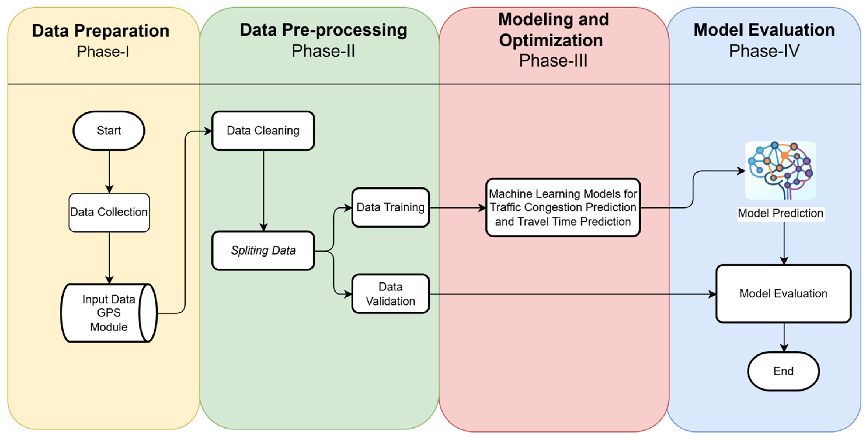
The system aims to predict traffic congestion and the arrival time of the BRT, allowing passengers to obtain estimated travel times for the bus through all stops on that route, as shown in Figure 1.

The process begins with Phase I: Data Understanding, where data are collected from GPS modules to serve as the foundation for analysis and modeling. This phase focuses on understanding data characteristics, including feature types and value distributions, to plan the next steps effectively. In Phase II: Data Preprocessing, the data undergo cleaning to remove errors and anomalies before being divided into training and testing subsets. The training data are used in Phase III: Modeling, where algorithms are applied to learn patterns and relationships for congestion and travel time prediction. The model is then evaluated using the testing data to ensure prediction accuracy. Finally, in Phase IV: Model Evaluation, the model’s performance and reliability are assessed using metrics such as the confusion matrix, R2 Score, MSE, RMSE, and MAE, ensuring that it meets the expected standards. The results are then analyzed to confirm the model’s readiness for practical implementation.

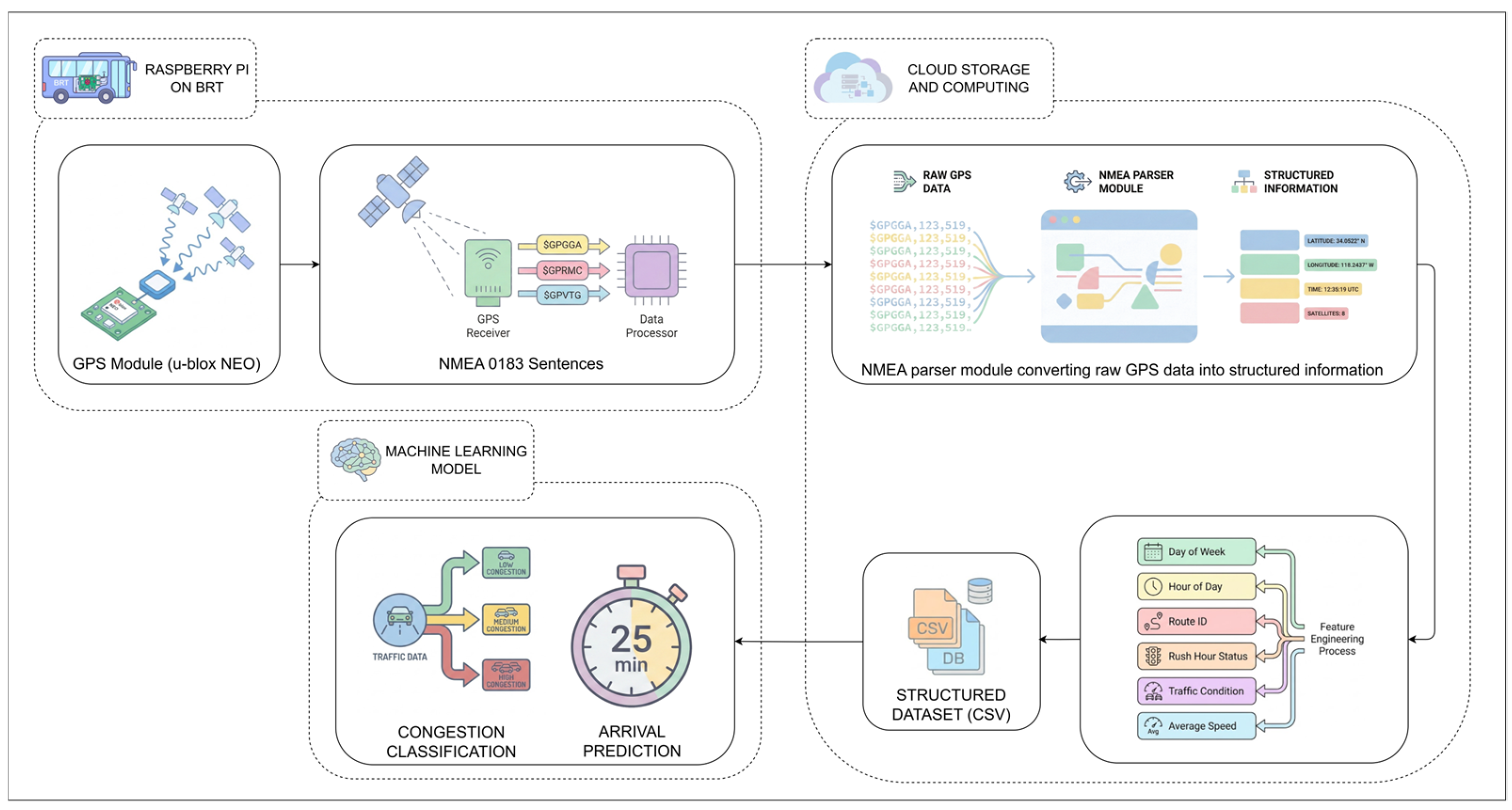
This system utilizes GPS-based datasets for both training and testing phases, with data acquisition performed directly on board Bus Rapid Transit (BRT) vehicles using a Raspberry Pi. As illustrated in Figure 2, a u-blox NEO GPS module installed on each bus continuously collects real-time positioning data and transmits raw location information in the form of NMEA 0183 sentences, including latitude, longitude, speed, and timestamp.

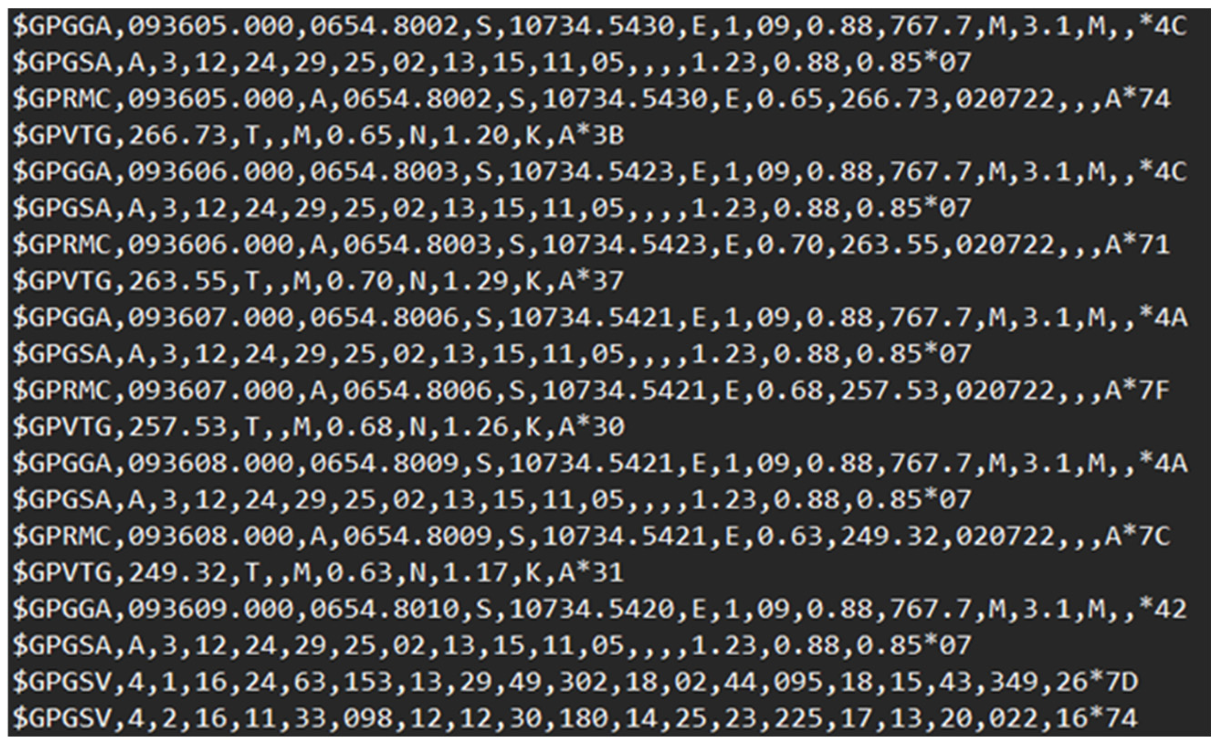
The raw NMEA data are received by the Raspberry Pi, which functions as an on-board data logger and preliminary processing unit. Once the GPS module is activated, the tracking process begins automatically and operates continuously while the bus is in service. The data collection process ends when the bus reaches the final terminal or completes its assigned route. During operation, the Raspberry Pi parses the NMEA sentences to extract relevant attributes and temporarily stores the data locally. The recorded GPS data are subsequently transmitted to a cloud-based storage and computing environment through a wireless connection. A VNC server platform is used to remotely access, manage, and monitor the datasets stored on both the Raspberry Pi and the cloud infrastructure. In the cloud processing stage, the parsed GPS data are converted from NMEA format into a structured CSV dataset as shown in Figure 3. The structured dataset undergoes data preprocessing, including data cleaning, validation, and feature engineering. Derived features such as temporal attributes (day of week and hour), route identifiers, rush-hour indicators, historical average speed per route, and traffic condition labels are generated to form a structured tabular dataset suitable for machine learning tasks.

These data are highly valuable for traffic condition analysis, particularly for identifying congestion patterns. Traffic congestion can be inferred from significant reductions in vehicle speed or prolonged stops occurring outside designated bus stops. Such events, identified through their spatial coordinates and temporal duration, serve as key indicators of congestion levels. Information regarding the location, duration, and severity of congestion is essential for understanding its impact on traffic flow. These insights support improvements in route smoothness, travel time estimation accuracy, and passenger comfort. Consequently, accurate identification of congestion patterns forms a critical foundation for subsequent predictive modeling and route optimization. Before the dataset is used for model training, several preprocessing steps are performed, including data conversion, data labeling, and handling missing values (NAN).

Table 1. Feature Engineering result.

Feature	Description	Type	Availability at Prediction Time
day	Day of week (1–7)	Categorical	Known (planned travel day)
hour	Hour of day (6–19)	Numerical	Known (planned travel time)
route	Bus route number (1–17)	Categorical	Known (selected route)
Rush_hours	Rush hour indicator (1 = 7–10 AM, 2 = other)	Binary	Known (derived from hour)
condition	Traffic condition (1 = Congested, 2 = Moderate, 3 = Smooth)	Categorical	Can be predicted from congestion model
avg_speed_route	Historical average speed per route	Numerical	Known (from historical data)

presents the results of this feature engineering process.

The dataset used in this study consists of a total of 20,156 records collected from GPS-based IoT devices installed on Bus Rapid Transit (BRT) vehicles operating in Bandung. Each record represents a spatiotemporal observation of a bus at a specific time and location. The dataset is structured in a tabular format and includes both temporal and operational features that are available at prediction time. The features comprise the day of the week, hour of the day, bus route identifier, rush-hour indicator, historical average speed per route, and traffic condition labels. Temporal features such as day and hour are known in advance based on planned travel schedules, while route information is selected by the user prior to prediction. The rush-hour indicator is derived from the hour attribute, and the historical average speed per route is obtained from previously collected data. Traffic condition labels are generated by the congestion classification model and can be used as input for travel time prediction. This structured dataset is designed to avoid data leakage by ensuring that all input features are either known or can be inferred at prediction time. With a total of 20,156 samples, the dataset provides sufficient coverage to train and evaluate machine learning models for both traffic congestion classification and travel time prediction tasks.

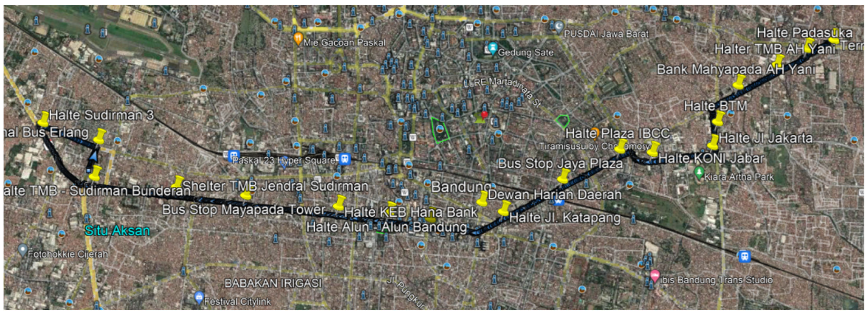
As shown in Figure 4, the departure route from Cicaheum Terminal to Cibeureum Terminal represents one of the main operational corridors of the Trans Metro Bandung (TMB) Bus Rapid Transit system. This corridor connects the eastern and western parts of Bandung City and passes through several strategic urban areas, including residential neighborhoods, commercial districts, and major arterial roads with high traffic activity. The route begins at Cicaheum Terminal and continues through multiple designated bus stops before terminating at Cibeureum Terminal. Each bus stop along this corridor serves as a critical passenger access point and contributes to variations in dwell time and traffic flow. Due to its alignment through central urban zones, the route is frequently affected by fluctuating traffic conditions, particularly during peak hours, which have a direct impact on travel time reliability and service efficiency.

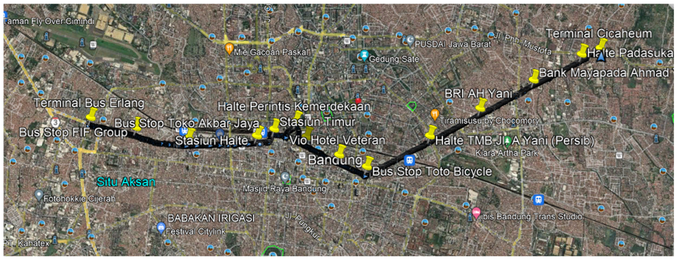
As shown in Figure 5, the departure route from Cibeureum Terminal to Cicaheum Terminal represents the return direction of the Trans Metro Bandung (TMB) Bus Rapid Transit corridor connecting the western and eastern parts of Bandung City. This route follows a different sequence of bus stops compared to the opposite direction due to traffic regulations and road geometry. The route starts at Cibeureum Terminal and proceeds through several designated bus stops before terminating at Cicaheum Terminal. Similar to the outbound route, this corridor passes through densely populated areas, commercial centers, and major arterial roads that are frequently affected by varying traffic conditions, especially during peak hours. These conditions influence bus travel time and service reliability.

At this stage, preprocessing continues until the data are ready for machine learning model creation. Categorical data are converted into numerical values to enable the regression process, as shown in Table 1 and

Table 2. Changes route to numeric.

Bus Routes	Numeric for Route
Cicaheum to Cibereum	1
Cibereum to Cicaheum	2

.

Based on Figure 4 and Figure 5, the departure and return routes differ, resulting in distinct bus stops for each direction. Numerical assignments are made accordingly, as shown in

Table 3. Cicaheum to Cibereum terminal.

Bus Routes	Numeric Halte
Terminal Cicaheum	0
Halte Padasuka	1
Halte AH Yani	2
Halte Bank Mahyapada	3
Halte BTM	4
Halte Jl Jakarta	5
Halte KONI	6
Halte Plaza IBCC	7
Halte Jaya Plaza	8
Halte Jl Ketapang	9
Halte HSBC	10
Halte Alun-Alun	11
Halte KEB Hana	12
Halte Mahaypada Tower	13
Halte Jendral Sudirman	14
Halte Bunderan Sudirman	15
Halte Jendral Sudirman 3	16
Terminal Elang	17

for the route from Cicaheum Terminal to Cibeureum Terminal, and

Table 4. Cibeureum to Cicaheum terminal.

Bus Routes	Numeric Halte
Terminal Elang	0
Halte FIF Group	1
Halte Toko Akbar Jaya	2
Halte Stasiun	3
Halte Stasiun Timur	4
Halte Perintis Kemerdekaan	5
Halte Bank CIMB	6
Halte Veteran	7
Halte Toto Bicycle	8
Halte Persib	9
Halte BRI AH Yani	10
Halte Bank AH Yani	11
Halte Padasuka 2	12
Terminal Cicaheum	13

for the route from Cibeureum Terminal to Cicaheum Terminal.

The route begins at Padasuka Stop (1) and continues to AH Yani Stop (2) along one of the city’s main arterial roads. The bus then passes Bank Mahyapada Stop (3) and BTM Stop (4) before reaching Jl. Jakarta Stop (5) and KONI Stop (6), both situated in one of the city’s busy activity centers. The route proceeds toward Plaza IBCC Stop (7) and Jaya Plaza Stop (8), which are located within commercial districts. In the midsection of the route, the bus stops at Jl. Ketapang Stop (9), followed by HSBC Stop (10) and the central city area at Alun-Alun Stop (11). The route then continues to KEB Hana Stop (12) and Mahaypada Tower Stop (13), which lie along the westbound segment of the corridor. Entering the Jenderal Sudirman area, there are three consecutive stops: Jendral Sudirman Stop (14), Bunderan Sudirman Stop (15), and Jendral Sudirman 3 Stop (16). The route concludes at Elang Terminal (17) as the endpoint on the western side.

Table 4 presents the ordered sequence of bus stops for the return route from Cicaheum Terminal to Cibeureum Terminal. This route consists of 14 stops, beginning at Elang Terminal, which is assigned the numeric value 0 as the starting point for the westbound journey.

The route begins at Elang Terminal (0), after which the bus proceeds to FIF Group Stop (1) and then to Toko Akbar Jaya Stop (2). Continuing along the corridor, the bus reaches Stasiun Stop (3), located near the central railway hub, followed by Stasiun Timur Stop (4), which serves the eastern side of the station area. The bus then continues toward Perintis Kemerdekaan Stop (5) before arriving at Bank CIMB Stop (6). As the route progresses into the city center, the next stop is Veteran Stop (7), which is situated in a busy commercial and governmental district. This is followed by Toto Bicycle Stop (8) and Persib Stop (9), both located within highly trafficked urban zones. In the eastern section of the route, the bus stops at BRI AH Yani Stop (10) and then Bank AH Yani Stop (11), which lie along one of Bandung’s major arterial roads. Nearing the end of the journey, the route reaches Padasuka 2 Stop (12) before terminating at Cicaheum Terminal (13) as the final stop. Overall, the structured numbering of the stops in Table 3 provides a clear representation of the reverse-direction corridor and can be used for route reconstruction, bidirectional mobility analysis, model validation, or integration into Machine Learning–based transport optimization frameworks.

After we obtained the data, the final step is create a model, which includes Random Forest and XGBoost algorithms that are validated and tested with an unseen dataset to evaluate its prediction accuracy for long-term dependencies. This evaluation provides an estimate of the model’s generalization ability in real traffic conditions. Evaluation metrics play a critical role in assessing model performance. The MAE measures prediction accuracy as the average absolute difference between predicted and actual values. The RMSE and MSE, commonly used metrics for regression tasks, weight errors according to their magnitude and are particularly sensitive to outliers in the data.

The MAE evaluates model performance by computing the average of the absolute differences between predicted and actual values. It provides a straightforward and easily interpretable measure of average error magnitude because its unit matches that of the original data. A significant advantage of MAE is its robustness to outliers; since it treats all errors linearly without squaring them, it avoids overemphasizing large deviations. The formula for MAE is given in (1).

$$MAE={\displaystyle \frac{1}{n}}{\sum }_{i=1}^n\left|y_i-\widehat{y_i}\right|$$

(1)

The MSE evaluates a model by calculating the average of the squared differences between predicted and actual values. Its key feature is that each error term is squared, which penalizes larger deviations more heavily. This property makes MSE sensitive to outliers, as even a single significant error can increase the overall score. Although its squared unit can reduce interpretability, MSE remains a standard metric for optimization during model training. The formula for MSE is given in (2).

$$MSE={\displaystyle \frac{1}{n}}{\sum }_{i=1}^n{\left(y_i-\widehat{y_i}\right)}^2$$

(2)

The RMSE is the square root of MSE. This metric resolves the interpretability issue by restoring the error’s unit to that of the original variable. Like MSE, RMSE penalizes significant errors more strongly and is sensitive to outliers, but its results are easier to interpret because they are expressed in the same unit as the target variable. The formula for RMSE is given in (3).

$$RMSE=\sqrt{{\displaystyle \frac{1}{n}}{\sum }_{i=1}^n{\left(y_i-\widehat{y_i}\right)}^2}$$

(3)

The R-squared (R²) score measures how well the independent variables explain the variance of the dependent variable. Its value ranges from 0 to 1, with a higher value indicating a better fit. The formula for the R² score is shown in (4).

$$R^2=1-{\displaystyle \frac{S{S}_{res}}{S{S}_{tot}}}=1-{\displaystyle \frac{{\sum }_{i=1}^n{\left(y_i-\widehat{y_i}\right)}^2}{{\sum }_{i=1}^n{\left(y_i-\overline{y}\right)}^2}}$$

(4)

3. Results and Discussion

3.1. Traffic Congestion Prediction

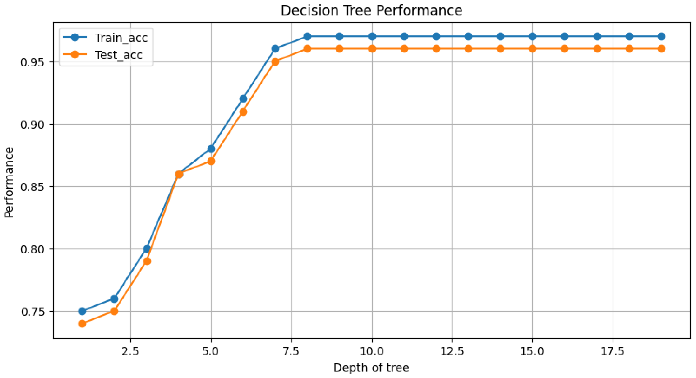
In this configuration, the dataset was divided into 80% training data and 20% testing data, comprising 16,124 samples for training and 4032 samples for testing. Model performance was evaluated using Precision, Recall, F1-score, and Accuracy metrics for both the Decision Tree and Random Forest classifiers. The Decision Tree and Random Forest models were evaluated to identify the optimal configuration that yields the highest classification accuracy for traffic congestion prediction. Model performance was assessed using the confusion matrix approach. During the training process, multiple experiments were conducted to determine the optimal value of the maximum depth hyperparameter. The maximum depth was analyzed by examining the training and testing accuracy across depth values ranging from 1 to 20. The maximum depth that resulted in the highest accuracy on the testing dataset was selected as the optimal model parameter. Figure 6 illustrates the training and testing accuracy curves obtained from the Decision Tree model for different maximum depth values.

As shown in Figure 6, the classification accuracy of the Decision Tree model increases as the tree depth increases, indicating enhanced learning capacity with greater model complexity. Both training and testing accuracy rise steadily from lower depth values and reach their peak at a tree depth of 8. Beyond this point, further increases in tree depth do not lead to significant improvements in testing accuracy, while the training accuracy remains relatively stable. Consequently, a maximum depth of 8 was selected as the optimal parameter for the Decision Tree model in this study.

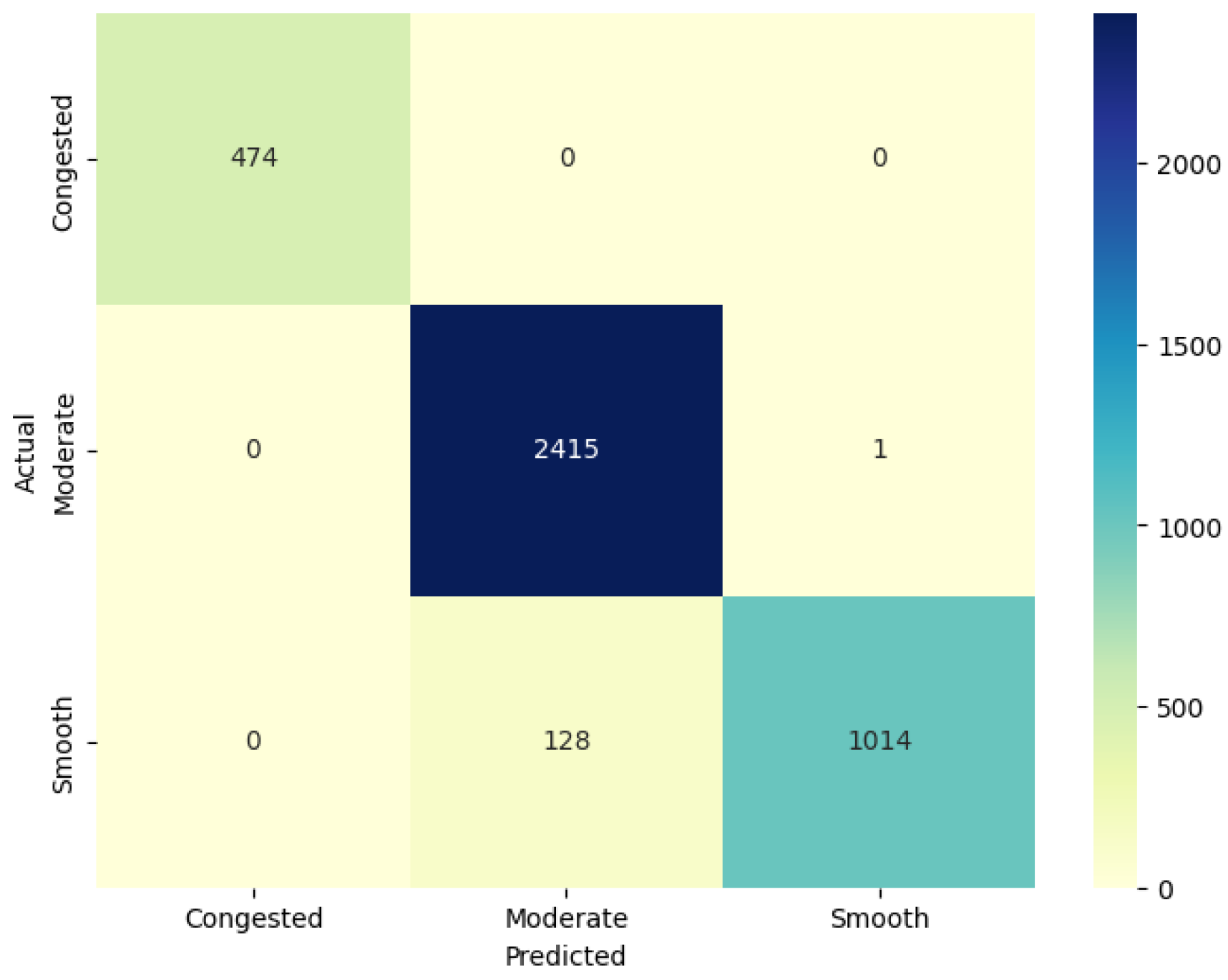
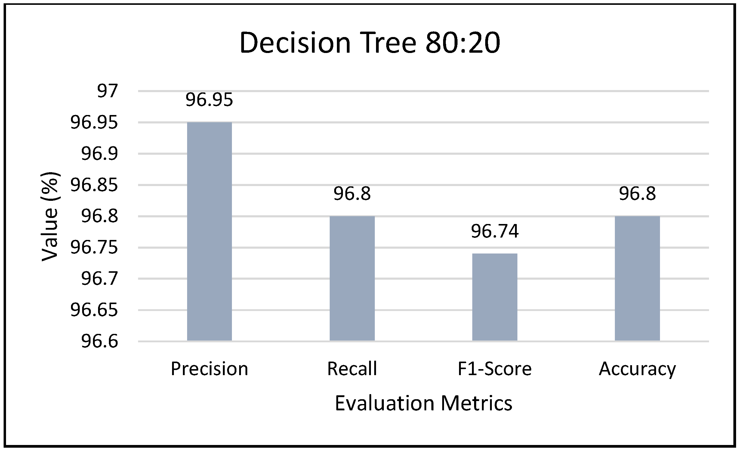
According to Figure 7, the Decision Tree model achieved strong classification performance across all congestion classes. For the Congested class, the true positive (TP) value was 474, with a false positive (FP) of 1 and no false negatives (FN = 0). For the Moderate class, the model recorded TP = 2415, FP = 128, and FN = 1, while for the Smooth class, TP = 1014, FP = 0, and FN = 128. Based on these confusion matrix values, the Decision Tree model attained a Precision of 96.9%, a Recall of 96.8%, an F1-score of 96.74%, and an overall Accuracy of 96.8% using a maximum depth of 8 with a random state of 0. The corresponding performance metrics, including precision, recall, F1-score, and accuracy, are illustrated in Figure 8.

These results demonstrate that the proposed model is capable of accurately classifying traffic congestion levels along bus routes, thereby supporting the identification of segments with lower congestion and enabling more reliable route planning and traffic management decisions.

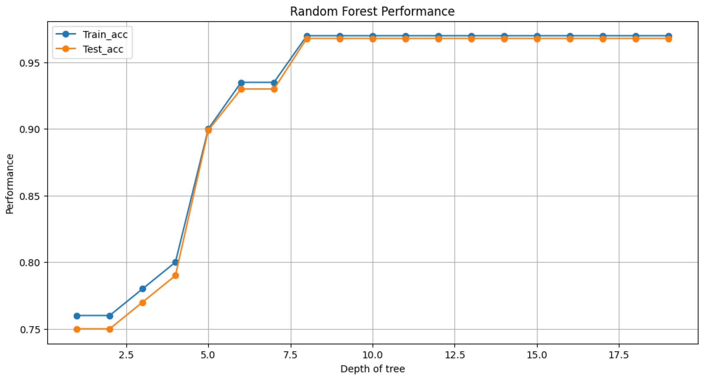
For the Random Forest model, Figure 9 illustrates the training and testing accuracy for traffic congestion prediction using an 80:20 data split. Similar to the Decision Tree model, the Random Forest classifier was evaluated by varying the maximum depth parameter to analyze its impact on model performance and generalization capability.

As shown in Figure 9, the training and testing accuracy of the Random Forest model increases as the maximum tree depth increases, indicating improved learning capability with greater model complexity. At lower depth values, both training and testing accuracy are relatively low, reflecting underfitting. As the depth increases, model accuracy improves rapidly and reaches a stable plateau at a tree depth of 8. Beyond depth = 8, further increases in tree depth do not lead to significant improvements in testing accuracy, while the training accuracy remains consistently high. The close alignment between training and testing accuracy across higher depth values indicates that the Random Forest model maintains good generalization performance and is less prone to overfitting due to its ensemble-based learning mechanism. The corresponding performance metrics are presented in Figure 10.

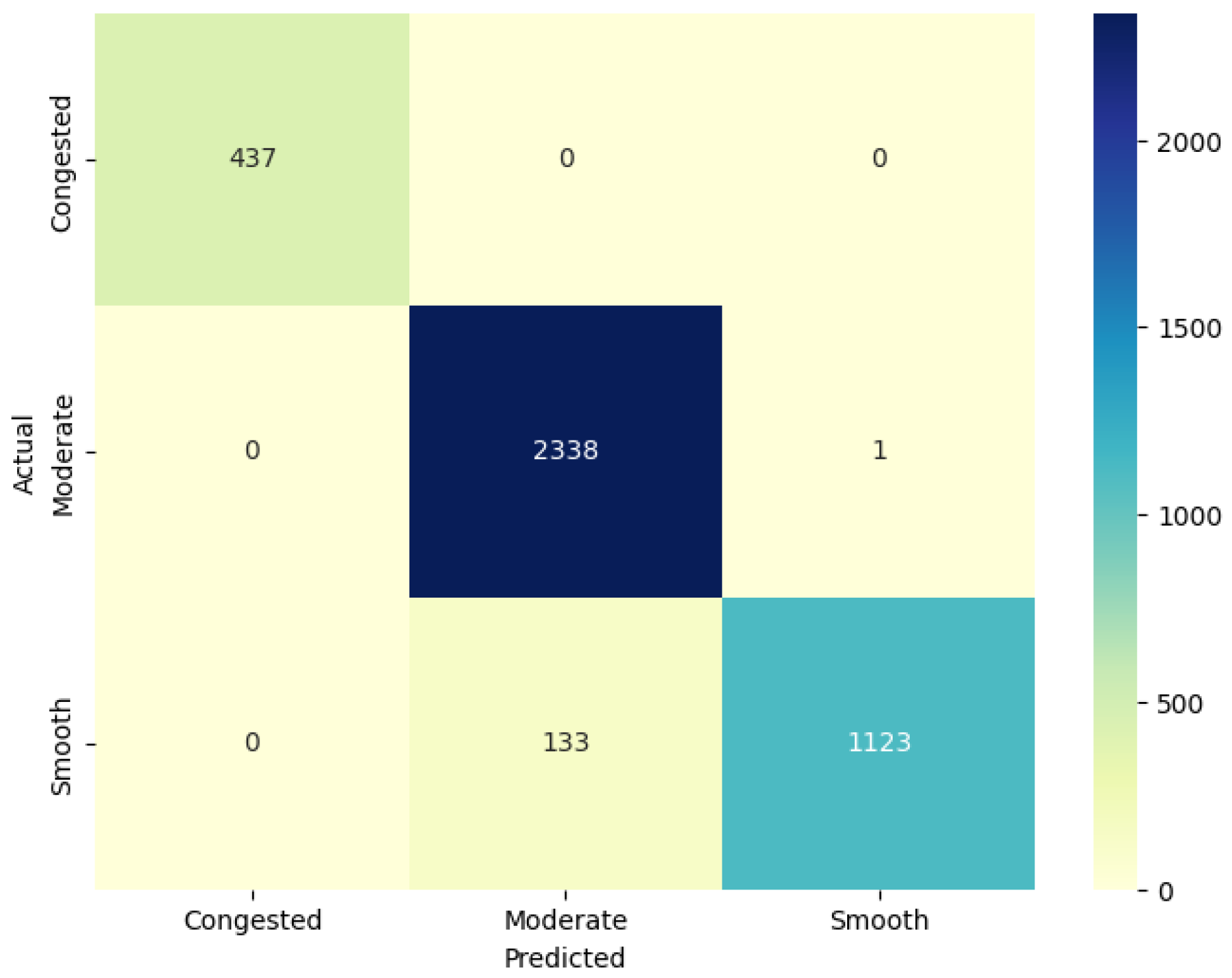
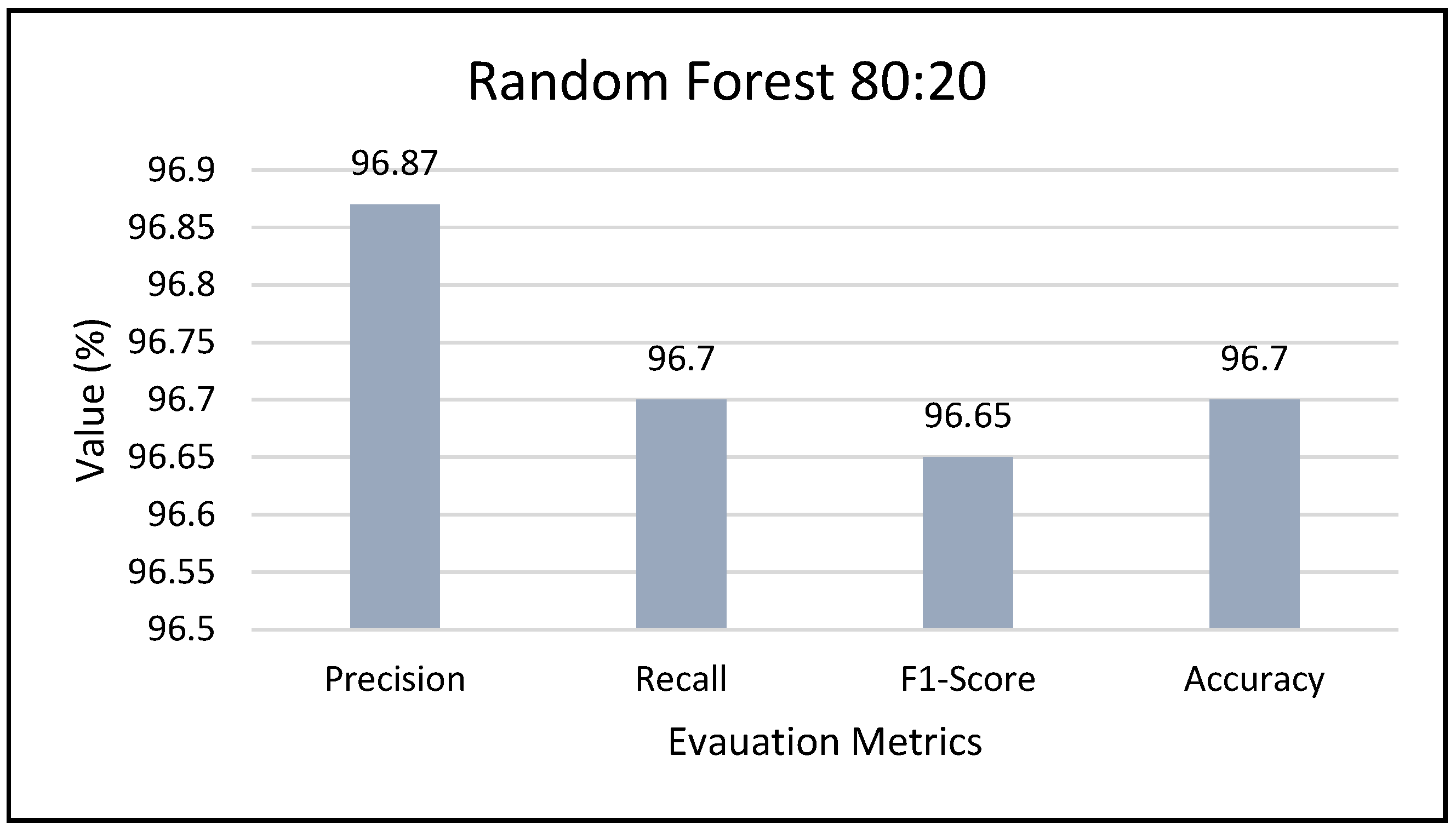
According to Figure 10, the TP value for the ‘Congested’ label is 437 with an FP value of 0 and an FN value of 0, while the TP value for the ‘Moderate’ label is 2338 with an FP value of 133, and an FN value of 1. Lastly, the TP value for the ‘Smooth’ label is 1123 with an FP value of 1 and an FN value of 133. Based on the obtained TP, FP, and FN values, the results for Precision, Recall, F1-Score, and Accuracy are shown in Figure 11. The Random Forest model has a precision of 96.87%, a recall of 96.7%, an F1-score of 96.65%, and an accuracy of 96.7%.

The results of both algorithms show that the prediction accuracy of congestion levels along travel routes is very high. Therefore, this approach can assist in identifying alternative routes with lower congestion levels. The confusion matrix method provides an effective means of evaluating accuracy by examining TP, FP, and FN values.

3.2. Travel Time

In this study, travel time is defined as the duration required for a bus to travel from the departure station to the destination station. The performance of the Random Forest and XGBoost regression models is analyzed to evaluate their ability to accurately estimate travel time, which represents one of the key operational challenges in the Bus Rapid Transit (BRT) system.

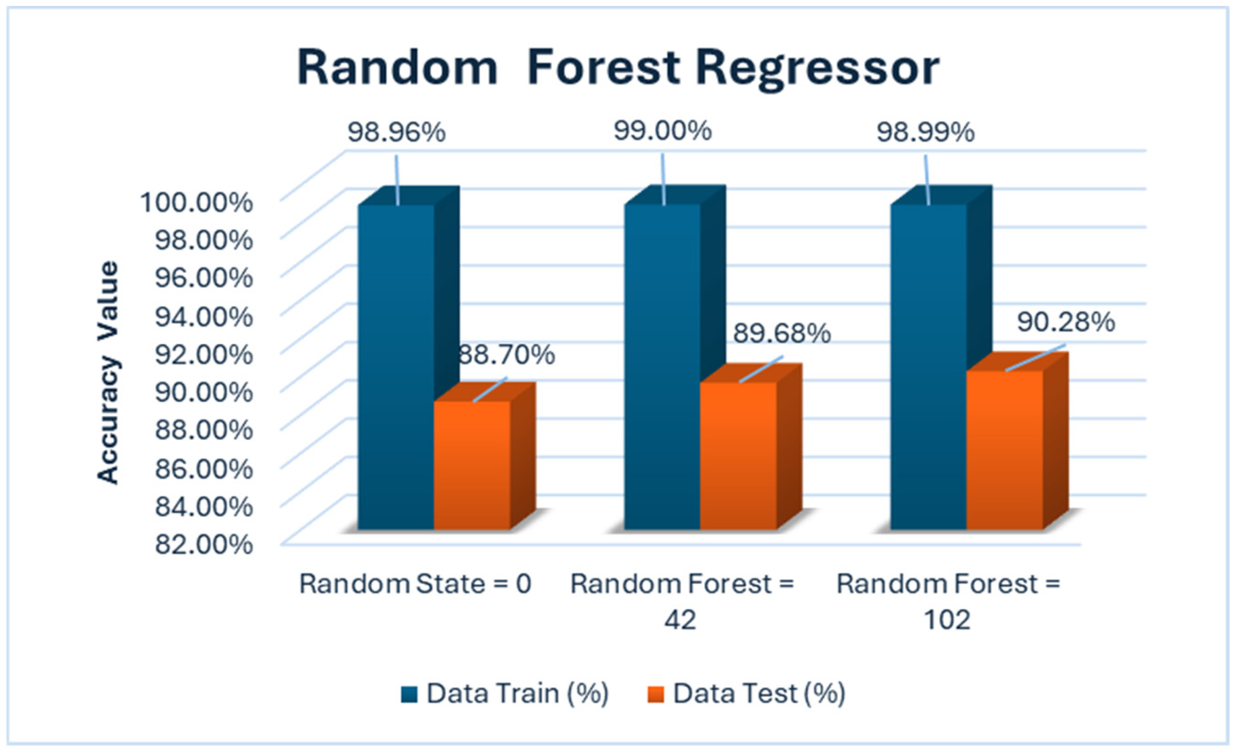
For model evaluation, both the Random Forest Regressor and XGBoost Regressor were tested using the same random state values (0, 42, and 102). The random state parameter was employed to ensure reproducibility of the experiments, rather than as a hyperparameter for performance optimization. The evaluation results of the Random Forest Regressor under different random states are presented in Figure 12.

As shown in Figure 12, the training and testing accuracy of the Random Forest Regressor were evaluated using three different random state values (0, 42, and 102) to ensure reproducibility of the experimental results. The training accuracy remains consistently high across all configurations, ranging from 98.96% to 99.00%, indicating that the model effectively captures the underlying patterns in the training data. For the testing data, the accuracy shows a gradual increase across different random state values. With random state = 0, the model achieves a testing accuracy of 88.70%. This value increases to 89.68% for random state 42 and reaches the highest observed testing accuracy of 90.28% for random state = 102. These variations are attributed to the inherent randomness in data sampling and model construction rather than changes in model capacity. These results indicate that the Random Forest Regressor demonstrates strong generalization capability in predicting travel time under consistent experimental settings.

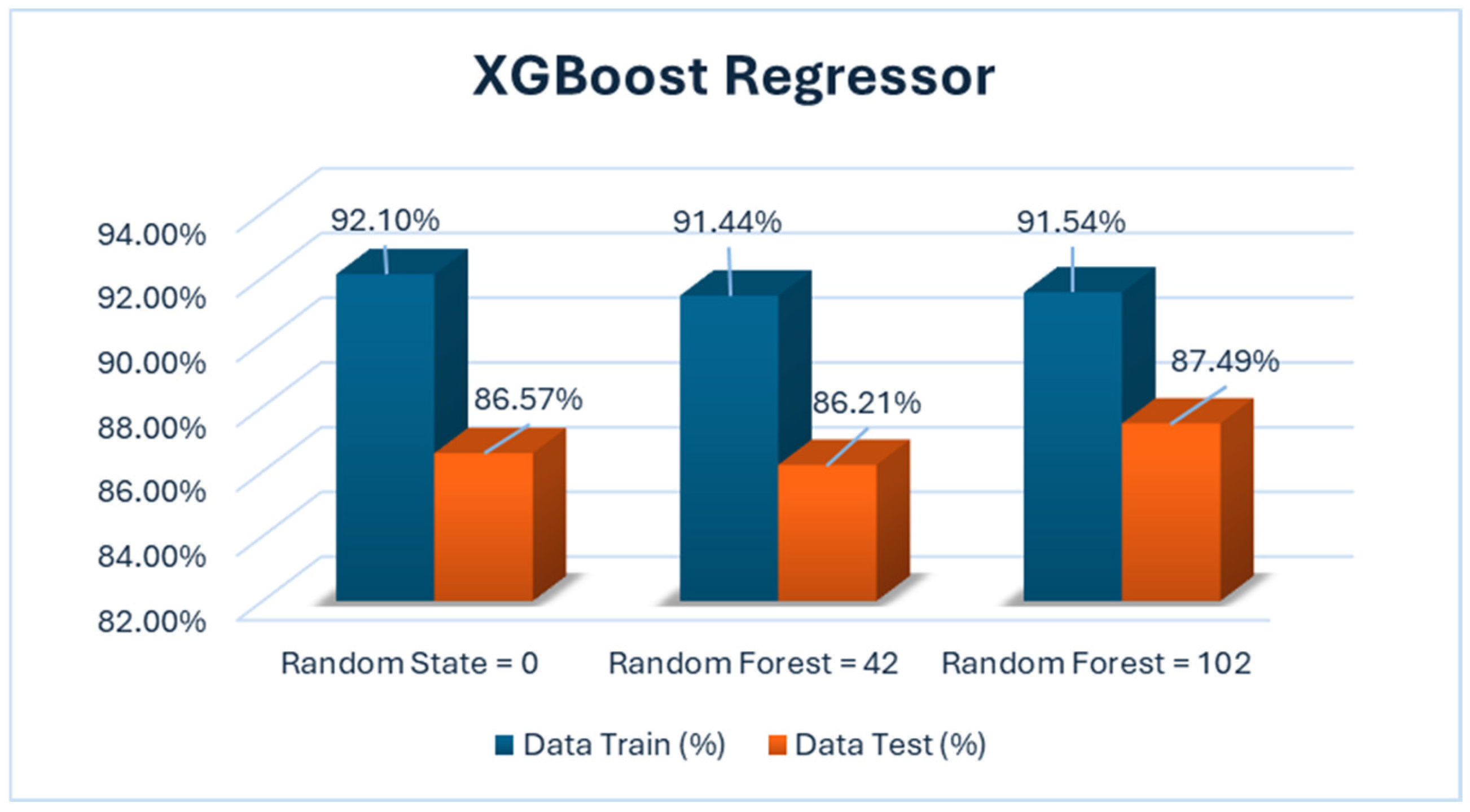
For the XGBoost Regressor, model performance was evaluated using the same random state values (0, 42, and 102) to ensure reproducibility and consistency of the experimental results. The random state parameter was used to control the inherent randomness in the training process rather than as a hyperparameter for optimization. The training and testing accuracy comparison for the XGBoost Regressor is presented in Figure 13.

As shown in Figure 13, the training and testing accuracy of the XGBoost Regressor were evaluated using three different random state values (0, 42, and 102) to ensure reproducibility of the experimental results. The training accuracy remains relatively stable across all configurations, ranging from 91.44% to 92.10%, indicating consistent learning performance of the model. For the testing data, the accuracy varies slightly due to the inherent randomness in data sampling and model initialization. The XGBoost model with random state = 0 achieved a testing accuracy of 86.57%, while random state 42 resulted in a testing accuracy of 86.21%. The highest observed testing accuracy of 87.49% was obtained with random state = 102. Despite these variations, all tested configurations achieve testing accuracy above 80%, demonstrating that the XGBoost Regressor exhibits stable and reliable generalization performance for travel time prediction. These results confirm that XGBoost is suitable for modeling travel time using real-world GPS-based IoT data, although its performance is slightly lower than that of the Random Forest Regressor in this study.

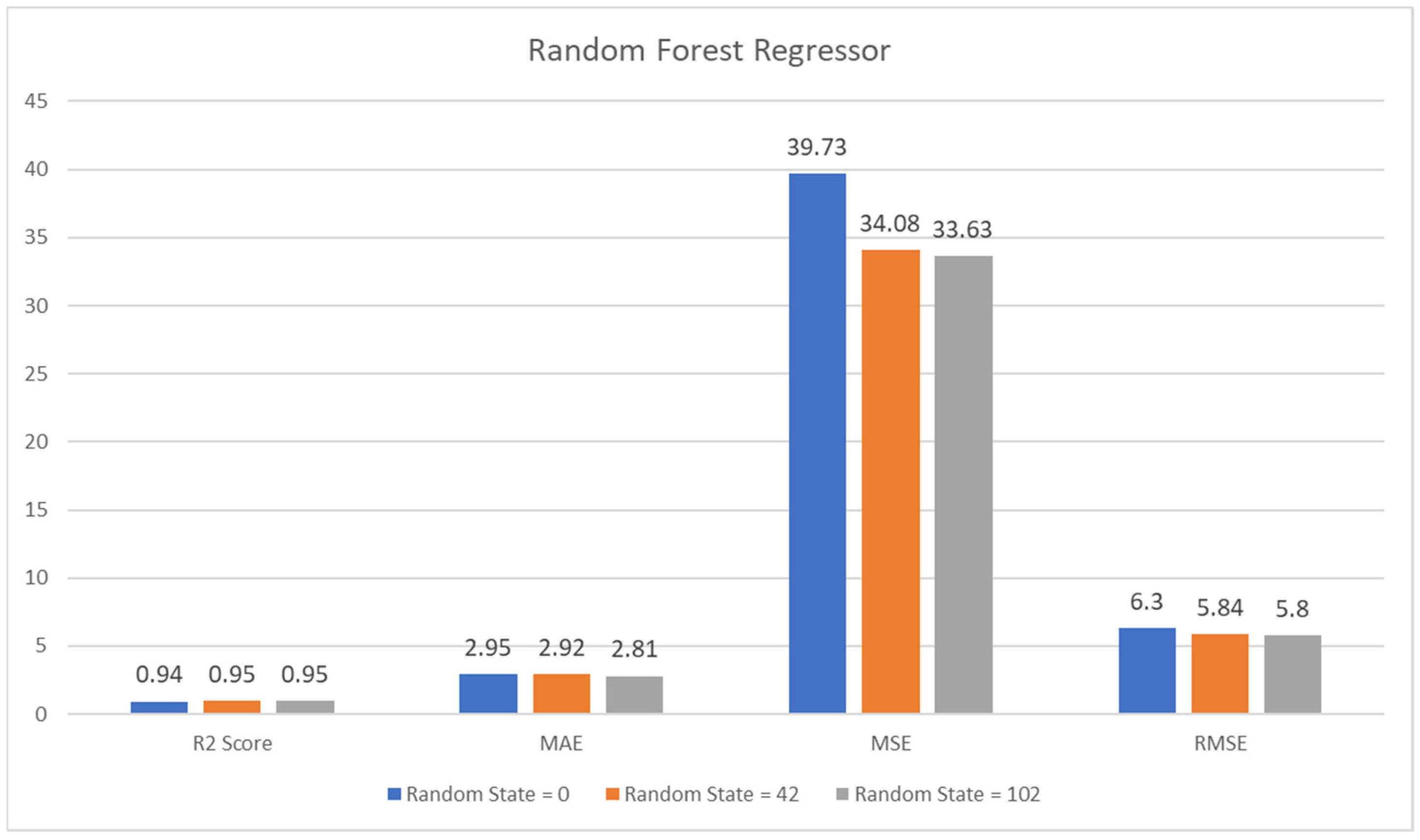
Figure 14 shows the results of R2 Score, MAE, MSE, and RMSE for the Random Forest Regressor Algorithm.

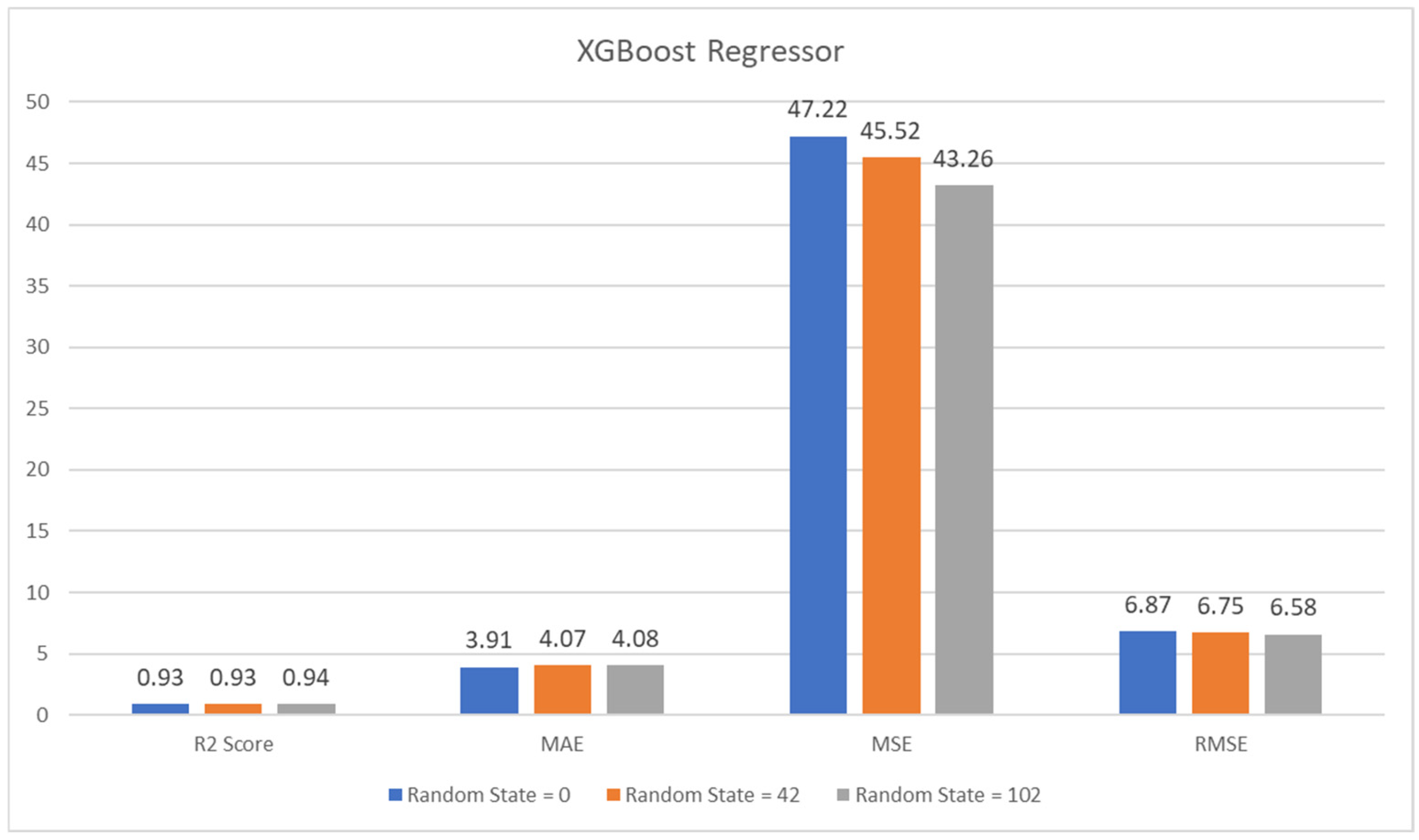
Figure 15 shows the results of calculating the R2, MAE, MSE, and RMSE scores for XGBoost Regressor.

XGBoost Regressor with Random state 102 achieved the highest R2 score in the error test, but for MAE, its performance was not as good as other random states. The lowest MSE value, 43.26, and the lowest RMSE value, 6.58, were obtained in the XGBoost 102 random state testing.

4. Discussion

The Random Forest algorithm has fewer errors than the XGboost algorithm in predicting travel time. Next, the training results will be tested using actual data.

Table 5. Actual time prediction data.

Route	Halte Early Stop	Halte Destination	Duration (Minute)
1	6	17	56.18
2	22	28	21.10
1	2	15	44.58
1	0	3	7.87
2	14	16	6.70

below contains the actual data. At this stage, a comparison will be made between the output results of the RF Regressor and XGBoost algorithms with the exact duration data.

In this scenario, a comparison will be made between the output results of the RF Regressor and XGBoost algorithms. This test aims to determine the differences in output results between these algorithms and the actual duration data. From the results obtained, it can be concluded that each algorithm produces differences in making predictions compared to the actual duration data. In

Table 6. Comparison of time prediction results.

Actual Time Prediction Data	Random Forest Prediction	XGBoost Regressor Prediction
56.18	47.15	57.68
21.10	21.64	21.36
44.58	47.42	49.80
7.87	7.64	10.87
6.70	9.10	9.84

, the RF algorithm in the first test has a relatively large difference where the actual data is 56.18 while the RF prediction result is 47.15. Similarly, in the third test, the actual data for the XGBoost algorithm was 44.58, while the prediction result was 49.80. In the fourth experiment, the actual data was 7.87, while the prediction result was 10.87. and the fifth experiment also shows a difference in output duration compared to the actual data, which is 6.70 in the actual data, while the prediction result is 9.84.

The duration results generated by the RF Algorithm with 98% accuracy are closer to the actual data than those generated by the XGBoost Algorithm with 92% accuracy.

Based on

Table 7. Comparison with another algorithm.

Model	Dataset	RMSE	MAE	MSE
LSTM [36]	METR-LA	6.78	5.12	45.96
ARIMA [36]	METR-LA	10.34	8.34	106.88
SVM [36]	METR-LA	8.72	6.78	76.06
MLP [36]	METR-LA	9.45	7.23	89.28
Random Forest	OUR DATASET	5.80	2.81	33.63

. The Random Forest Model using our dataset demonstrated the best performance with an RMSE of 5.80, MAE of 2.81, and MSE of 33.63, indicating high prediction accuracy. LSTM also showed good performance with an RMSE of 6.78, MAE of 5.12, and MSE of 45.96, though it was slightly below Random Forest. In contrast, ARIMA had the lowest performance with an RMSE of 10.34, MAE of 8.34, and MSE of 106.88. The SVM and MLP models were positioned in the middle; SVM had an RMSE of 8.72, MAE of 6.78, and MSE of 76.06, while MLP had an RMSE of 9.45, MAE of 7.23, and MSE of 89.28. Overall, Random Forest was the most superior model among all the models compared.

5. Conclusions

The conclusions drawn from this study are as follows: The 80:20 data split was chosen as the best data split because it is considered to be resistant to new data. For congestion prediction results, the Decision Tree model achieved a testing accuracy of 96.8% compared to the random forest, which only achieved an accuracy of 96.7%. This means that Decision Tree has better accuracy than Random Forest. Meanwhile, for travel time prediction, the Random Forest machine learning model achieved an accuracy of 98.96%, while the XGBoost algorithm achieved an accuracy of 92.10% when tested using actual data. When testing the prediction results with actual data for travel time, the Random Forest algorithm’s prediction results were more consistent with the duration in the actual data than the XGBoost algorithm’s prediction results. The Random Forest model performance evaluation produced an RMSE value of 5.80, which is the smallest error value, so the machine learning model is considered to improve accuracy and reduce error values for traffic congestion and BRT bus fleet travel time problems. Therefore, the models to be implemented on the website system are the Decision Tree algorithm for Congestion Prediction and Random Forest for Travel Time prediction. Although limited in terms of corridor coverage and feature complexity, this study provides a methodological foundation for cities in developing countries to replicate economical smart transportation systems while opening opportunities for future enhancements through the integration of weather data, incident information, and more advanced algorithms to further improve urban mobility.

To improve this research, several future improvements are proposed. The predictive model can be refined by adding features such as bus location visualization and route recommendations on demand. In addition, key areas for future research involve implementing this model on portable devices and IoT-based platforms. This will enable continuous, real-time monitoring of the transportation system. This approach will provide users with practical and instant assessments of transportation conditions, thereby increasing the usability and effectiveness of the system.

References

1. Berawi, M.A.; Sari, M.; Amiri, N.H.A.; Susilowati, S.I.; Utami, S.R.; Kulachinskaya, A. Developing a Machine Learning Model to Improve the Accuracy of Owner Estimate Cost in the Capital Expenditure Procurement Process. Int. J. Technol. 2025, 16, 1179. [Google Scholar] [CrossRef]
2. Noorsaman, A.; Amrializzia, D.; Zulfikri, H.; Revitasari, R.; Isambert, A. Machine Learning Algorithms for Failure Prediction Model and Operational Reliability of Onshore Gas Transmission Pipelines. Int. J. Technol. 2023, 14, 680–689. [Google Scholar] [CrossRef]
3. Abduljabbar, R.; Dia, H.; Liyanage, S. Machine Learning Traffic Flow Prediction Models for Smart and Sustainable Traffic Management. Infrastructures 2025, 10, 155. [Google Scholar] [CrossRef]
4. Devi, S.; Neetha, T. Machine Learning based traffic congestion prediction in a IoT based Smart City. Int. Res. J. Eng. Technol. 2017, 4, 3442–3445. Available online: www.irjet.net (accessed on 23 December 2025).
5. Megantara, E.; Munadi, R.; Sussi. Arrival Time Prediction Bus Trans Metro Bandung with Internet of Things and Machine Learning Method. e-Proceeding Eng. 2022, 8, 3801–3806. Available online: https://openlibrarypublications.telkomuniversity.ac.id/index.php/engineering/article/view/19124 (accessed on 25 December 2025).
6. Visconti, P.; Rausa, G.; Del-Valle-Soto, C.; Velázquez, R.; Cafagna, D.; De Fazio, R. Innovative Driver Monitoring Systems and On-Board-Vehicle Devices in a Smart-Road Scenario Based on the Internet of Vehicle Paradigm: A Literature and Commercial Solutions Overview. Sensors 2025, 25, 562. [Google Scholar] [CrossRef]
7. Shi, Z.; Wang, Y.; Guo, D.; Jiao, F.; Zhang, H.; Sun, F. The Urban Intersection Accident Detection Method Based on the GAN-XGBoost and Shapley Additive Explanations Hybrid Model. Sustainability 2025, 17, 453. [Google Scholar] [CrossRef]
8. Abdi, A.; Amrit, C. A review of travel and arrival-time prediction methods on road networks: Classification, challenges and opportunities. PeerJ Comput. Sci. 2021, 7, e689. [Google Scholar] [CrossRef]
9. Sarrab, M.; Pulparambil, S.; Awadalla, M. Development of an IoT based real-time traffic monitoring system for city governance. Glob. Transit. 2020, 2, 230–245. [Google Scholar] [CrossRef]
10. Liu, D.; Sun, J.; Wang, S. BusTime: Which is the Right Prediction Model for My Bus Arrival Time? In Proceedings of the 2020 5th IEEE International Conference on Big Data Analytics (ICBDA 2020), Xiamen, China, 8–11 May 2020; pp. 180–185. [Google Scholar] [CrossRef]
11. Grinsztajn, L.; Oyallon, E.; Varoquaux, G. Why do tree-based models still outperform deep learning on typical tabular data? Adv. Neural Inf. Process. Syst. 2022, 35, 507–520. [Google Scholar]
12. Sakib, N. Machine Learning-based Travel Time Prediction Models for Complex Traffic Conditions. SSRN 2024. [Google Scholar] [CrossRef]
13. Champahom, T.; Banyong, C.; Janhuaton, T.; Se, C.; Watcharamaisakul, F.; Ratanavaraha, V.; Jomnonkwao, S. Deep Learning vs. Gradient Boosting: Optimizing Transport Energy Forecasts in Thailand Through LSTM and XGBoost. Energies 2025, 18, 1685. [Google Scholar] [CrossRef]
14. Gifty, A.; Li, D.Y. A Comparative Analysis of LSTM, ARIMA, XGBoost Algorithms in Predicting Stock Price Direction. Eng. Technol. J. 2024, 9, 4978–4986. [Google Scholar] [CrossRef]
15. Pan, X. The Comparison Between Random Forest and LSTM Models Based on the Gold Price Prediction. Adv. Econ. Manag. Polit. Sci. 2024, 94, 102–108. [Google Scholar] [CrossRef]
16. Sujatha, R.; Teja, A.; Naveen, P.; Chatterjee, J.M.; Aarthy, S.L.; Hassanien, A.E. Web application for traffic monitoring and guidance. J. Syst. Manag. Sci. 2020, 10, 1–14. Available online: https://www.aasmr.org/jsms/Vol10/Vol.10.4.3.pdf (accessed on 25 December 2025).
17. Nivaan, G.V.; Tomasila, G.; Suyoto. Smart bus transportation for tracking system: A study case in Indonesia. In IOP Conference Series: Earth and Environmental Science; IOP Publishing: Philadelphia, PA, USA, 2021; Volume 729. [Google Scholar] [CrossRef]
18. Khan, M.A.; Khan, S.F. IoT based framework for Vehicle Over-speed detection. In Proceedings of the 2018 1st International Conference on Computer Applications & Information Security (ICCAIS), Riyadh, Saudi Arabia, 4–6 April 2018; pp. 1–4. [Google Scholar] [CrossRef]
19. Oladimeji, D.; Gupta, K.; Kose, N.A.; Gundogan, K.; Ge, L.; Liang, F. Smart Transportation: An Overview of Technologies and Applications. Sensors 2023, 23, 3880. [Google Scholar] [CrossRef]
20. Shingare, A.; Chaudhari, N.; Deshpande, P. GPS Supported City Bus Tracking & Smart Ticketing System. In 2015 International Conference on Green Computing and Internet of Things (ICGCIoT); IEEE: New York, NY, USA, 2015; pp. 93–98. [Google Scholar]
21. Sousa, P.M.E.S., Jr.; Costa, D.F.; Coutinho, E.F.; Bezerra, C.I.M. An IoT solution for monitoring and prediction of bus stops on university transportation using machine learning algorithms. In Proceedings of the 10th Euro-American Conference on Telematics and Information Systems, Fortaleza, Brazil, 12–15 November 2020. [Google Scholar] [CrossRef]
22. Sarker, M.R.A.; Hassanuzzaman, M.; Biswas, P.; Dadon, S.H.; Imam, T.; Rahman, T. An efficient surface map creation and tracking using smartphone sensors and crowdsourcing. Sensors 2021, 21, 6969. [Google Scholar] [CrossRef]
23. Soori, M.; Arezoo, B.; Dastres, R. Internet of things for smart factories in industry 4.0, a review. Internet Things Cyber-Phys. Syst. 2023, 3, 192–204. [Google Scholar] [CrossRef]
24. Miranda, W.M.; De Mendonça, R.T.R.; Da Silva, A.A.; De Lima Curvello, A.M.; De Souza, F.L.D.S.; Da Silva, H.J. BusMe: Automatic Bus Localization System and Route Registration. Procedia Comput. Sci. 2017, 109, 1098–1103. [Google Scholar] [CrossRef]
25. Al-Hawari, F.; Al-Sammarraie, M.; Al-Khaffaf, T. Design, validation, and comparative analysis of a private bus location tracking information system. J. Adv. Transp. 2020, 2020, 8895927. [Google Scholar] [CrossRef]
26. Priandani, N.D.; Tolle, H.; Yunianto, D.R. Design and implementation of mobile-based application for Malang City public transportation route search. Int. J. Adv. Soft Comput. Appl. 2016, 8, 48–58. [Google Scholar]
27. Martín, J.; Khatib, E.J.; Lázaro, P.; Barco, R. Traffic monitoring via mobile device location. Sensors 2019, 19, 4505. [Google Scholar] [CrossRef] [PubMed]
28. Sun, S.; Chen, J.; Sun, J. Traffic congestion prediction based on GPS trajectory data. Int. J. Distrib. Sens. Netw. 2019, 15, 1550147719847440. [Google Scholar] [CrossRef]
29. Satrinia, D.; Saptawati, G.A.P. Traffic speed prediction from GPS data of taxi trip using support vector regression. In Proceedings of the 2017 International Conference on Data and Software Engineering (ICoDSE), Palembang, Indonesia, 1–2 November 2017; Volume 2018, pp. 1–6. [Google Scholar] [CrossRef]
30. Ashwini, B.P.; Sumathi, R.; Sudhira, H.S. A Dynamic Model for Bus Arrival Time Estimation based on Spatial Patterns using Machine Learning. Int. J. Eng. Trends Technol. 2022, 70, 185–193. [Google Scholar] [CrossRef]
31. Mousa, S.; Ishak, S. Comparative evaluation of tree-based ensemble algorithms for short-term travel time prediction. arXiv 2018, arXiv:1810.10102. [Google Scholar]
32. Qiu, B.; Fan, W. Machine learning based short-term travel time prediction: Numerical results and comparative analyses. Sustainability 2021, 13, 7454. [Google Scholar] [CrossRef]
33. Huang, H.; Huang, L.; Song, R.; Jiao, F.; Ai, T. Bus Single-Trip Time Prediction Based on Ensemble Learning. Comput. Intell. Neurosci. 2022, 2022, 6831167. [Google Scholar] [CrossRef]
34. Firdaus, D.; Munadi, R.; Purwanto, Y. DDoS Attack Detection in Software Defined Network using Ensemble K-means++ and Random Forest. In 2020 3rd International Seminar on Research of Information Technology and Intelligent Systems (ISRITI); IEEE: New York, NY, USA; pp. 164–169. [CrossRef]
35. Khan, N.; Ullah, F.U.M.; Afnan; Ullah, A.; Lee, M.Y.; Baik, S.W. Batteries State of Health Estimation via Efficient Neural Networks with Multiple Channel Charging Profiles. IEEE Access 2021, 9, 7797–7813. [Google Scholar] [CrossRef]
36. Mahajan, D.; Pottigar, V.V.; Suresh, C.; Fahad, A. Implementing Real-Time Traffic Flow Prediction Using LSTM Networks for Urban Mobility Optimization. Commun. Appl. Nonlinear Anal. 2025, 32, 01–27. [Google Scholar] [CrossRef]
Figure 1. Workflow for predicting arrival time.
Iot 07 00022 g001
Figure 2. System Design.
Iot 07 00022 g002
Figure 3. NMEA data from GPS as a dataset.
Iot 07 00022 g003
Figure 4. Departure route from Cicaheum terminal to Cibeureum terminal.
Iot 07 00022 g004
Figure 5. Departure route from Cibeureum terminal to Cicaheum terminal.
Iot 07 00022 g005
Figure 6. Training and testing accuracy of the Decision Tree model based on different maximum depth values.
Iot 07 00022 g006
Figure 7. Results of the Confusion Matrix for Decision Tree 80:20 Ratio.
Iot 07 00022 g007
Figure 8. Confusion Matrix Value Graph for Decision Tree 80:20 Ratio.
Iot 07 00022 g008
Figure 9. Training and testing accuracy of the Random Forest model based on different maximum depth values.
Iot 07 00022 g009
Figure 10. Results of the Confusion Matrix for Random Forest 80:20 Ratio.
Iot 07 00022 g010
Figure 11. Confusion Matrix Value Graph for Random Forest 80:20 Ratio.
Iot 07 00022 g011
Figure 12. Random Forest Regressor Accuracy.
Iot 07 00022 g012
Figure 13. XGBoost Regressor Accuracy.
Iot 07 00022 g013
Figure 14. Random Forest error rate.
Iot 07 00022 g014
Figure 15. XGBoost error rate.
Iot 07 00022 g015