Abstract
In this short review, we focus on some of the subjects, related to J. Cleymans’ pioneering contribution of statistical approaches to the particle production process in heavy-ion collisions. We discuss these perspectives from the effects of stochastic processes in collective variables of hydrodynamic description, which is described by a stochastic variational method. In this connection, we stress also the necessity of the inclusion of surface and quantum effects in the study of relativistic heavy-ion reactions.
1. Introduction
The history of hydrodynamic description goes back to even before the 18th Century, and as we know, it has been applied widely to the studies of continuum media in many different scenarios. In fact, the hydrodynamic approach works not only for the description of a variety of phenomena around us, but also for the systems in completely different scales, from elementary particles to the Universe. As a microscopic example, the relativistic hydrodynamic approach is an important tool for the study of the properties of the matter produced in relativistic heavy-ion collisions. There, the properties of the matter created in these processes are reflected in the behaviors of collective flow variables [1,2,3,4,5,6]. On the other hand, as a macroscopic example, hydrodynamic modeling has been an indispensable tool in the studies of astrophysical phenomena. More recently, in particular, a full general relativistic hydrodynamics is required in the investigation of the so-called multi-messenger astrophysics such as neutron star or black hole mergers; see, e.g., [7].
The above wide range of the applicability of the hydrodynamic description comes from the fact that its basic kinematic structure is nothing but a set of local conservation laws, such as energy, momentum, charges, etc., and expressed in the forms of the equations of continuity. Of course, the proper definitions of the local conserved densities and the continuum assumption depend on systems and are not always trivial. These may enter some subtle aspects, as we discuss below. However, once the system is represented as a continuum medium in the form of local conserved densities and its flows, the corresponding equations of continuity are applicable independently of the properties and size of the matter. This is the principal reason why the hydrodynamic approach can have a wide applicability irrespective of the scale of the system.
On the other hand, it is evident that the set of these equations of continuity alone does not form a closed system to describe dynamics. They are simply kinematic constraints for the dynamical evolution of continuum media. To describe the time evolution, we have to introduce “forces” in a closed form: these forces should be specified as functions (or functionals) of conserved densities. For example, in the case of an ideal fluid description, any infinitesimal part of the fluid is assumed to stay in thermodynamic equilibrium adiabatically during the whole time evolution. In such a case, the force is simply given by the pressure, which is a function of other local densities.
As sketched above, the hydrodynamic description requires several assumptions and also depends on the external input, such as the equation of state (EoS). Thus, the hydrodynamic description is basically phenomenological. Even its most fundamental assumption of the continuum medium for the matter is not always justified in a quantitative manner. This becomes pronounced in the applications to microscopic systems such as relativistic heavy-ion collisions. As described below, the applicability of hydrodynamics is intimately related to the concept of coarse-graining procedure through which we introduce the local densities of the medium and corresponding thermodynamic properties.
To clarify the concept of the coarse-graining procedure, let us consider, as an example, the statistical model for the particle productions in heavy-ion collisions. In this model, we consider the whole ensemble of produced particles in a huge number of collisional events, within a certain kinematic domain. By assuming the grand-canonical ensemble, this system is characterized by a few thermodynamic parameters, such as temperature and chemical potentials. These parameters can be adjusted to reproduce the relative abundance of different species. This statistical approach in heavy-ion collisions indicates new mechanisms of particle productions, such as Hagerdorn’s prediction of the limiting temperature in hadronic gas, J/ suppression, strangeness enhancement, and thermal photon and lepton pair signals [8,9,10,11,12,13,14,15,16,17,18,19,20]. These observations converged to the idea of the formation of quark–gluon plasma (QGP), in the early 2000s.
The relativistic hydrodynamic description of the dynamics of QGP is nothing but a more microscopic and dynamical version of the statistical model. In fact, this is literally the most microscopic system of fluid ever known [21] (see English translation in [22]). There, instead of identifying a unique hot QGP fireball as the average over many collisional events, we consider that such a hot and dense state of the QGP stage is created initially in the small domain at the instant of the collision and develops as a fluid in spacetime. The time evolution of the hot QGP depends on the different initial condition defined on an event-by-event (EbE) basis. This is a natural step toward the spacetime description of the QGP, starting from the statistical model.
In the case of relativistic heavy-ion collisions, however, the proper system is microscopic so that the spacetime evolution of the QGP fluid is not observable directly in experiments. For a given experimental event, we only know a few pieces of global information, which characterizes the initial condition of two colliding nuclei and the momentum distribution of the produced particles with their identification in the final state. Thus, to apply the hydrodynamic description under such a restrictive condition, we introduce three distinct steps in practice: (1) preparation of hydrodynamic initial conditions from the particle system, (2) hydrodynamic evolution, and (3) particlization from the fluid final state. In the first step, we usually rely on the use of a some well-established event generator based on nucleon–nucleon high-energy collisions. Then, the initial distributions of the energy and the momentum are constructed for a given collision geometry of the colliding nucleus, which is characterized by, for example, the impact parameter (see also the discussion below). This is done by a smoothing procedure over the energy, the momentum, and the location of primordial particles produced in each event generator. In this paper, we refer to such a procedure as geometric coarse graining.
Once the initial condition is determined, in the second step, we follow its hydrodynamic evolution until the assumptions of the hydrodynamic description are violated. For example, if the density of the fluid becomes less than a certain critical value, the fluid description is considered to be invalid. The hypersurface in the four-dimensional spacetime where the fluid attains the critical density is called the freeze-out surface. In the third step, the final fluid state on the freeze-out surface is mapped into the corresponding momentum distribution of the produced particles, in terms of the so-called freeze-out process. Technically speaking, the freeze-out mechanism involves complicated physical mechanisms, such as the chemical and thermal freeze-out, after-burner, etc, but we do not enter into the details here.
The above steps are repeated to generate an ensemble of many “hydrodynamic collisional events” for a specific collision geometry. In a nucleus–nucleus collision, the basic parameters for a collision geometry are the impact parameter (collision centrality) and the corresponding collisional plane. We identify the simulated event ensembles as that of the corresponding experimental events classified by the same collisional geometry in a statistical sense. From this identification, we can calculate statistical correlations of observables in both ensembles and compare them. Such correlations can characterize non-trivial signals of the presence of collective motions as dynamic responses of the QGP matter. Here, we stress that the EbE analysis does not mean the one-to-one correspondence between a hydrodynamic simulation and experimental data in an individual collisional event. We rather suppose that the ensemble of the hydrodynamic events is statistically equivalent as a whole to the corresponding experimental events. This is a kind of coarse-graining procedure in the identification of observables. For simplicity, we refer to this procedure as the statistical coarse-graining. This EbE hydrodynamic analysis was first introduced in [23].
As described above, a hydrodynamic approach in the heavy-ion collisions focuses on the collective flow of the system, introducing some coarse-graining procedures of different natures. The collective features in collisional events are reflected in the characteristic correlations among detected particles. Some observables are known to be related directly to the global initial condition geometry (such as impact parameter and collision plane) and others to those EbE fluctuations, e.g., the local inhomogeneities. The EbE analysis has revealed that the fluctuations in the initial conditions with the same class of the global geometry manifest themselves in the collective flow observables, such as , , establishing hydrodynamic natures.
Here, we stress again that the determination of correlations among observables requires the ensemble average over different events with a specified initial global geometry. Therefore, strictly speaking, the success of the hydrodynamic description does not necessarily mean that all assumptions behind it are justified literally as they are. In the hydrodynamic description, we assume that the QGP is formed as a continuum medium represented by an ensemble of small domains, called fluid elements. They should be specified by a set of local conserved densities in thermodynamic equilibrium, at least approximately. For this to happen, the size of a fluid element must be orders of magnitude smaller than that of the whole fluid, but at the same time, it should be sufficiently dense so that it contains a huge number of the QGP particles. In addition, the local thermal relaxation time must be sufficiently shorter than the time scale of the hydrodynamic evolution to keep the fluid element in a state close to the thermal equilibrium during its evolution. However, as mentioned, we are not considering one-to-one correspondence between the two ensembles, hydrodynamic evolutions, and experimental events, and hence, the observables contain the statistical coarse-graining. In this sense, the hydrodynamic description for the rather global collective flow parameters, such as , , are insensitive to more local dynamics of the system. To investigate the more detailed behavior of the QGP dynamics, nonlinear correlations should be analyzed since there are different initial conditions that reproduce the same collective flow parameters. For example, the distinction of finite flows between a global triangular anisotropy and the presence of a hot spot in the peripheral region is not clear [24,25]. The measurements of higher-order correlations in observables will further refine these questions with respect to the coarse-graining scale, and such efforts are being made by studying the non-linear response of the collective parameters [26,27].
Up to now, we have not considered the presence of viscosity, which is of course an important factor for the hydrodynamic description. In ideal hydrodynamics, the fluid elements are thermally equilibrated during the time evolution and smoothly connected to their neighbors. Their time evolution should be adiabatic, and the total entropy is conserved. In such a case, it is well known that the hydrodynamic equation of the system is equivalent to the set of classical equations of motion of each fluid element. The so-called Lagrange coordinate system faithfully reflects such an image. Then, it is rather straight to see that we can apply the variational method to derive the hydrodynamic equations, defining the action of the system simply introducing the internal energy of each fluid element. As is known, the variational approach has many advantages in formulating the dynamical problem in an elegant and transparent way to deal with, e.g., the relation between the conservation laws and symmetries. As an example, ideal relativistic hydrodynamic equations are derived from the same action, just written in a covariant form [28].
From the variational point of view, ideal hydrodynamics describes the optimal trajectory of the fluid elements, where they interact with the neighbors exchanging the internal energy in an adiabatic way. Then, if we follow this image to deal with dissipative processes, we need to include the non-adiabatic processes in the interactions among the fluid elements. This is not trivial in a self-contained variational scheme without introducing an artificial modification such as Rayleigh’s dissipation function.
One possibility is to extend the domain of dynamical variables as classical deterministic ones by introducing stochastic variables in the definition of the action. This is a natural way to include the fluctuations associated with the coarse-graining mechanism. Such a generalized variational method is known as the stochastic variational method (SVM) [29,30,31,32]. In this review, we focus our attention on some known systems where the SVM approach is applicable. The action is defined as the average over the whole ensemble of stochastic events. The variation is taken with respect to these stochastic dynamical variables, whose initial and final conditions are specified in terms of their distributions.
The original motivation of the SVM was to derive the Schrödinger equation in terms of noises around the classical trajectory [29], but the SVM approach is shown to be valid to derive viscous hydrodynamics, as well. It is shown that the Navier–Stokes and Gross–Pitaevskii, in addition to the generalized diffusion equations are derived within the framework of the SVM [33]. There, the quantum uncertainties and uncertainties in hydrodynamic descriptions due to the coarse-graining procedure are dealt with by the same framework [32,34,35,36]. The crucial point of the SVM approach compared to the ordinary variation method is that we deal with the non-differentiability and the time-reversed stochastic trajectories.
This paper is organized as follows. In Section 2, we describe the essential structure of the stochastic variational approach and discuss several known results, such as the derivation of the Schrödinger equation. In Section 3, we apply the SVM to the system of fluids and derive generalized viscous hydrodynamics. In Section 4, we discuss the roles of the new term, which does not appear in standard viscous hydrodynamics. This term, on the one hand, plays a crucial role for quantum-mechanical systems and, on the other hand, generates the surface tension in generalized viscous hydrodynamics. In Section 5, we discuss the uncertainty relation in hydrodynamics. The application to curved geometric systems is discussed in Section 6. Section 7 is devoted to concluding remarks.
2. Stochastic Variation Method
Let us consider a single-particle system with mass m. In the standard variational principle of classical mechanics, it is known that the physical particle trajectory is given by the optimized path of the action:
where and are the initial and final times and dot denotes the time derivative. The Lagrangian, L, is defined by
where the potential energy is denoted by . There, it is implicitly assumed that the virtual trajectories for variation are differentiable. Then, as known, the optimized path of the action is given by the solution of the Newton equation. If we permit considering, however, non-differential virtual trajectories in the variational procedure, the optimized dynamics could be modified from the Newton equation. The SVM is one such generalized variational method.
The typical example of non-differentiable trajectories is found in the Brownian motion. In a manner analogous to this, in the SVM, the particle trajectory is assumed to be given by the following forward stochastic differential equation (SDE):
where is a time-dependent vector field to be determined, and is given by the standard Wiener process, satisfying
where symbol denotes the Kronecker delta, and , stay for the component index of space-like vectors. The ensemble average for the Wiener process is denoted by . The intensity of the stochasticity is characterized by the parameter .
The standard definition of velocity in classical mechanics is not applicable in stochastic trajectories because the left-hand and right-hand limits of a zigzag path do not agree. To accommodate this ambiguity, we consider also the backward time evolution of the trajectory described by the backward SDE:
where represents another standard Wiener process. The vector function is determined from using the consistency condition, discussed below.
Nelson introduced two different time derivatives [37]: one is the mean forward derivative and the other the mean backward derivative , which are defined by
Here, the expectation value is the conditional average for fixing , and we used the fact that is Markovian.
The two unknown vector functions are not independent. To see this, let us introduce the particle distribution, which is defined by
where denotes the initial position of the stochastic particle, and its distribution is characterized by . Applying the forward and backward SDEs to this definition, two Fokker–Planck equations are obtained ():
To conform Equation (8) to Equation (7), should be chosen to satisfy the consistency condition:
A more general representation of the consistency condition is shown in Equation (25) of [32]. It is also noteworthy that these Fokker–Planck equations are reduced to the same equation of continuity:
where the mean velocity field is defined by
To apply the stochastic variation to the single-particle Lagrangian (2), one needs to replace with and of Equation (6). Suppose that the kinetic term of the Lagrangian is replaced with the average of the two time derivatives. Then, the single-particle stochastic Lagrangian is defined by
Let us define the variation of the stochastic trajectory by
where is an infinitesimal function satisfying
The stochastic variation of the stochastic Lagrangian (12) leads to the stochastic Euler–Lagrange equation:
Substituting Equation (12), one finds:
Note that is described by the equation of continuity (10).
The above result, Equation (16), of the stochastic variation can be cast into a more familiar form. Let us introduce a complex function, defined by
where the phase, , is defined by
The evolution equation of is obtained from Equation (16), and then, satisfies
When
is chosen, Equation (19) becomes the Schrödinger equation; here, ℏ is the reduced Planck’s constant. Then, actually, Equation (16) coincides with the so-called Madelung’s hydrodynamic representation of the Schrödinger equation.
3. Generalized Viscous Hydrodynamics
In Section 2 above, it is shown that quantization is the stochastic optimization of the classical action. That is, when we observe a single-particle system with a macroscopic scale where the non-differentiability of the particle trajectory becomes negligibly small, we can apply the classical variation to the single-particle action, and the Newton equation is obtained. However, if the system has a microscopic scale, one has to optimize the corresponding action with the stochastic variation, and the Schrödinger equation is derived. In this sense, we can understand that classical mechanics emerges as the result of the coarse-graining caused by large differences in scales of observables.
Let us apply this idea to another example of coarse-graining in hydrodynamics. The behavior of the ideal fluid is described by the Euler equation, while that of the viscous (Newtonian) fluid is described by the Navier–Stokes–Fourier (NSF) equation. In an ideal fluid, the local thermal equilibrium is perfectly satisfied for each fluid element during their time evolution. Therefore, the thermodynamic property of the fluid elements changes in a quasi-static manner. In other words, the time scale of the collective dynamics of an ideal fluid is much longer than the local relaxation time for thermal equilibrium. On the other hand, when the fluid changes in a relatively smaller scale, there exist small deviations from the thermal equilibrium in the internal states. Since this deviation is not represented by a function of thermodynamic quantities, the fluid obtains extra acceleration mechanisms attributed to the non-equilibrium nature of the fluid elements. Therefore, one can consider that the difference between the Euler and NSF equations comes from that of the coarse-graining in the spacetime scale in the hydrodynamic behavior. In such a smaller scale, the trajectories of the fluid elements are not always smooth, as is the case of the Schrödinger equation. If this idea is correct, one can obtain the NSF equation from the Euler equation by using the stochastic variation.
As mentioned in the Introduction, the motion of a fluid can be represented by the ensemble of the motions of fluid elements. We consider a simple fluid composed of N constituent particles with mass m. The Lagrangian of the system is given by the sum of the contributions from each fluid element as
where is the Lagrange coordinate of the fluid element. Each fluid element involves a fixed number of constituent particles, which is conserved in the time evolution. Then, the initial distribution of the fluid elements is characterized by , normalized by N,
The internal energy per particle in the fluid element at time t is denoted by and given as . Here, is the internal energy density and is the number density of the constituent particles of the fluid element at time t for a given initial position .
Applying the classical variation to this Lagrangian, one obtains the Euler equation, which describes the motion of the ideal fluid:
where
In the Lagrange coordinates moving with the fluid elements of the ideal fluid, the specific entropy of each fluid element is constant. Thus, the quantity (24) can be identified with the thermodynamic pressure,
where s is the specific entropy of the fluid element. The detailed mathematical derivation of the pressure term in the variation is shown in [32].
Let us apply the stochastic variation to the ideal classical Lagrangian (21). As was mentioned in the derivation of the Schrödinger equation, there is an ambiguity for the replacement in the kinetic term of the stochastic Lagrangian, and we simply assumed that the stochastic kinetic term is given by the average of the contributions of and . Here, we consider a more general situation. Suppose that the kinetic term is given by the most general quadratic form of , defined in Equation (6),
where
and and are real parameters. In the vanishing limit of the noise, , the two mean derivatives are reduced to the standard time derivative, and thus, the kinetic term (26) coincides with the classical kinetic term,
Using this, the general form of the stochastic Lagrangian, corresponding to Equation (21), is given by
The stochastic variation finally leads to the following equation,
where the traceless symmetric stress tensor is defined by
The shear viscosity and the bulk viscosity are defined by
The second coefficient of viscosity, , emerges from the variation of through the changes of the associated specific entropy, as suggested in [33]. One can find that Equation (30) is identical to the NSF equation,
except for the term that contains , which is discussed in Section 4 below.
Here, the stochastic optimization of the averaged behavior of fluid dynamics was considered in terms of the fluctuating motion of the fluid element. It is however possible to consider models, where the noise terms are added directly to hydrodynamics; for recent studies, see [38,39] (and references therein).
4. Quantum Effects and Surface Energy
The coefficient is defined by
This does not appear in the NSF equation (33), but one can immediately notice that it turns out to be the quantum potential term by choosing . Indeed, Equation (30) is sometimes used as a model of a quantum viscous fluid [40,41].
The appearance of the term in generalized hydrodynamics has been discussed for a long period of time. For example, Brenner pointed out that, since the velocity of a tracer particle of a fluid is not necessarily parallel to the mass velocity, the existence of these two velocities should be taken into account in the formulation of hydrodynamics. This theory is called bivelocity hydrodynamics [32,34,42,43,44], and Equation (30) is understood to be one of the variants.
Another example is related to the diffuse-interface models of hydrodynamics [45]. The properties of the interface between two fluids has been studied since the 19th Century by Young, Gauss, Maxwell, Gibbs, Rayleigh, van der Waals, and others. In particular, Korteweg [46] considered that the behavior of liquid–vapor fluids near phase transitions is described by the Navier–Stokes–Korteweg (NSK) equation, and our Equation (30) is its special case. Then, the term describes the capillary action; for more details, see review [45].
As a matter of fact, the term is related intimately to the surface tension and can be incorporated into the classical Lagrangian. Modifying the internal energy term of the Lagrangian Equation (21) as
the classical variational approach leads to the term in the equation of motion Equation (30) without the viscous term (). This type of internal energy was introduced in the Thomas–Fermi model for the nuclear density distribution, showing the relation between the term and the surface energy for a saturating system, such as nuclear matter [47,48].
To illustrate the role of the noise in the SVM formulation as the surface energy, let us consider the hydrostatic equilibrium of a fluid with such a term in the Lagrangian. The density distribution at the hydrostatic equilibrium for a given total number of constituent particles is given by
where
and
is the total number of particles. Here, the number density should be non-negative and is the Lagrangian multiplier (chemical potential). Applying the usual variational procedure with respect to the density , we readily obtain the following differential equation for the spherical symmetric case,
where r is the radial coordinate and
In order to satisfy the boundary condition for at i.e., , Equation (37) should be solved as an eigenvalue problem of for a given value of central density .
For a system such as nuclear matter, the internal energy par particle as a function of is characterized by the following properties:
where is the equilibrium density for an infinite matter and is the maximum density due to the strong repulsive forces at close distances between particles (hard core). As an example, let us consider the following function:
where is a positive constant with the dimension of energy.
Figure 1 shows the radial dependences of the number density, , which are given by the eigenfunctions of Equation (37) by setting . The result is plotted by using an adimensional radial variable . The solid, dotted, and dashed lines correspond to , and , respectively. The line for corresponds to the infinite homogeneous matter in its hydrostatic equilibrium. These density distributions show the plateau in the central bulk domain and the exponentially decreasing surface. Thus, these distributions are reminiscent of the known Wood–Saxon distribution for the nuclear density. The surface thicknesses of the three lines are almost constant and scaled by the value of . Indeed, because of the definition of x, one can easily see that the larger , the wider the surface thickness. Due to the practically vanishing radial derivative except for the surfaces, the positive contribution of the term in Equation (35) comes basically from the surfaces that have almost the same thickness for the three lines. Therefore, to minimize the energy fixing the total N, the area of the surface should be reduced. This is the reason why the central density increases for a smaller N.
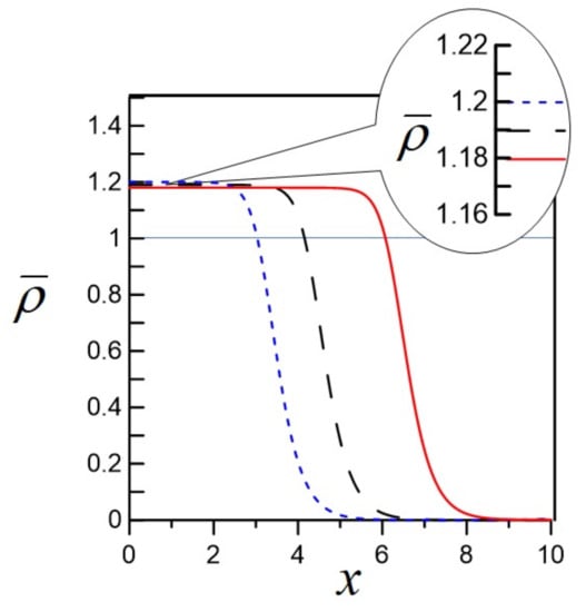
Figure 1.
The radial dependences of the number density, obtained by solving Equation (37). Here, , , and is set. The solid, dotted, and dashed lines correspond to , and , respectively. The line corresponds to the infinite homogeneous matter in its hydrostatic equilibrium. See text for details.
5. Uncertainty Relation in Hydrodynamics
The uncertainty relations characterize an important feature in quantum physics, and its comprehension requires unceasing improvement. Recently, the present authors proposed a new formulation of the uncertainty relations, which reproduce quantum mechanical results and are also applicable to general stochastic dynamics within the framework of SVM [34]. Using this, one can derive the uncertainty relations for the motion of the fluid element of a viscous (Newtonian) fluid.
To illustrate the method, let us consider the single-particle stochastic Lagrangian (12), which is applied to obtain the Schrödinger equation. In this Lagrangian, the two time-derivatives are introduced and are attributed to the non-differentiability of the stochastic trajectories. Then, two momenta are introduced through the Legendre transformation of the stochastic Lagrangian:
Here, the factor 2 in the definitions is introduced for a convention to reproduce the classical result in the vanishing limit of .
The standard deviation of position of a quantum particle is defined by
where , the following expectation value is introduced:
where N is the normalization factor of analogous to Equation (22) and is a unity, , for quantum mechanics of single particle system, and D denotes the number of the spatial dimension. The standard deviation of momentum is defined by the average of the two standard deviations:
Using these definitions and the Cauchy–Schwarz inequality, we can show that the product of and satisfies the inequality [34]:
where is defined by Equation (11). The second term on the right-hand side of Equation (42) is expressed in terms of the quantum-mechanical notation:
where and are the position and momentum operators, respectively, and denotes the expectation value with a wave function. With this identification, one finds that Equation (42) is the Robertson–Schrödinger inequality. When the second term on the right-hand side is ignored, this becomes the Kennard inequality.
The advantage of the present approach compared to the standard canonical formulation is that it is easily extended to the generalized coordinates systems. Let us consider the generalized coordinate, , and the corresponding canonical momentum, . Then, the uncertainty relation in the generalized coordinates system is given by [35]
where J is the Jacobian of the generalized coordinates and is the Christoffel symbol. The term next to on the right-hand side gives a finite contribution when is a periodic variable. Actually, for the angle variable in the polar coordinates, this is reduced to
where L is the angular momentum. For the eigenstate of the angular momentum, the right-hand side vanishes, . The above inequality resolves the famous problem in the angular uncertainty relation.
In the above calculations, the lower bound of the inequality is due to the consistency condition (9), which comes from the consistency between the forward and backward SDEs. That is, the finite minimum uncertainty is attributed to the non-differentiability of trajectories. Therefore, the similar inequality should be satisfied for the motion of the fluid element in viscous hydrodynamics. We now apply the same procedure to the Lagrangian of generalized viscous hydrodynamics (29). Different from the quantum-mechanical case, we consider the motion of the fluid element. Thus, the uncertainty relation in this application reads the restriction for the fluctuating motion of the fluid element. Then, the uncertainty relation for the fluid element of generalized viscous hydrodynamics [32,34] is given by
where m is the mass of the constituent particle of a simple fluid and is the kinematic viscosity
Different from the quantum-mechanical case, the minimum uncertainty on the right-hand side of the inequality (46) is not a constant, but a function of thermodynamic variables through viscosity. For the case of the NSF equation (33), where , one can find that the uncertainty will be enhanced for larger viscosity.
In the same inequality (46), the right hand side shows that the minimum uncertainty of the inviscid fluid is modified by the effect of viscosity. It is natural to assume that the minimum uncertainty of the inviscid fluid is larger than the quantum-mechanical minimum, . Suppose that the viscous effect does not improve uncertainty beyond the inviscid (and thus quantum-mechanical) minimum. To satisfy this condition, the kinematic viscosity has the following lower bound [35]:
This lower bound is the same order of magnitude as the Kovtun–Son–Starients (KSS) bound of the shear viscosity [49]. This may suggest the close relation between the KSS bound and the minimum uncertainty relation. See also [50].
In quantum mechanics, it is known that the minimum uncertainty state is given by the coherent state. Even in viscous hydrodynamics, one can write down the minimum uncertainty state, which is given by the generalized coherent state; for details, see [35].
6. Quantum Mechanics in Curved Spacetime
The framework of the SVM is applicable to particle systems described by generalized coordinates in curved geometries. For this application, the modification of the noise term in the SDEs is crucial. For example, suppose that the forward SDE for the radial component in the polar coordinates is expressed by the direct generalization of Equation (3):
where is the Wiener process. This equation however does not function because can take any real value at random, and thus, the positivity can be violated.
In the following, we discuss a non-relativistic SVM system in the curved geometry following the formulation developed in [51,52]. Let us consider a curved spacetime geometry characterized by the metric where is a function only of time, and the indices denoted by the Greek letters stay for the time (0) and space (1,2,3) components. Moreover, there is no mixture terms of the spacetime components, . The position in this generalized coordinates is denoted by . On the other hand, one can find local Minkowskian coordinates around , which is denoted by . The Minkowskian metric is . The Latin indices etc. stay for the local Minkowskian coordinates, etc. are reserved to denote the spatial components of . Then, one can introduce the tetrads, defined by
These tetrads satisfy
where the convention of taking summation for repeated indices is used. The forward SDE in generalized coordinates is given by
where c denotes the speed of light, and the Stratonovich definition of the product is introduced:
for an arbitrary smooth function . Since is defined in the local Minkowskian coordinates, one can use the same Wiener process been applied so far. The backward SDE is defined in a similar way; see [51,52] for details.
Let us consider the single-particle system of mass m, which is described by the following stochastic Lagrangian:
where and V is a potential energy. Here, the kinetic term is expressed by the average of the two contributions, and . For the case of more general replacement, one obtains the viscous term [52].
The stochastic variation then leads to
where , , and are the covariant derivative, the Laplace–Beltrami operator, and the Ricci tensor , respectively. The four-velocity field is defined by
The probability density satisfies the equation of continuity,
The remarkable feature of Equation (58) is the last term on the right-hand side, which is induced by the interplay between quantum fluctuation and spacetime curvature. We call this the quantum-curvature (QC) term. To investigate the role of this term, is set. Then, taking the limit of the flat spacetime, Equation (58) is reduced to Madelung’s hydrodynamic representation of the Scrödinger Equation (16). To express the above result in terms of the wave function, we have to obtain the equation of the phase of the wave function from Equation (58). This is impossible in general due to the -dependence of . That is, no wave function can be introduced to express quantum dynamics in general geometries. It should be emphasized that, normally, the existence of the Hilbert space is required from the beginning of quantization, but this is not trivial a priori.
However, if the Ricci tensor is a constant, then one can still introduce the wave function, while the corresponding Schrödinger equation becomes non-linear. For example, let us set
Then, the wave function can be defined as , and the Schrödinger equation is given by [51]
The linearity of quantum mechanics is violated by the QC term.
When the standard Friedmann-Lemaitre-Robertson-Walker FLRW metric is considered, the QC term becomes a negative pressure term in the energy–momentum tensor. However, it was found that the magnitude of the negative pressure is extremely smaller than the accepted value from the observations; see [51] for details.
There are attempts to gain new insights for the interplay between quantum fluctuation and curved geometry in laboratories. For example, the Bose–Einstein condensate is regarded as an analogue black hole [53,54,55]. The quantum superposition of spacetime geometries will be observed through the gravitational entanglement of mesonic particles, which is called the Bose–Marletto–Vedral (BMV) effect [56,57,58]. The toy model considered here can be applied to study these kinds of phenomena.
Quantum mechanics in curved space is normally formulated based on the Hilbert space, and hence, one may wonder whether the appearance of the non-linear term above is an artifact of the SVM procedure. In [59,60,61], Nelson’s stochastic mechanics is extended to curved systems. To satisfy the linearity of the Schrödinger equation, the adapted parallel transport of stochastic quantities violates the length conservation of the transported vector. In the present approach, the stochastic variational principle is required as a fundamental requirement of quantization, maintaining this length conservation.
7. Summary and Future Challenges
In the present paper, the stochastic variational approach (SVM) was reviewed. The SVM naturally reproduces the viscous stress tensor under the stochastic optimization of the action of the ideal fluid. In addition, by considering the forward and backward time evolutions of stochastic trajectories, the consistency condition for the stochastic trajectories necessarily leads to a new acceleration term, which is identified with the quantum (Bohm) potential in a microscopic system. Therefore, the SVM can be considered as a natural framework to formulate viscous hydrodynamics incorporating the quantum effects.
The term, corresponding to the quantum potential, appears in the applications to macroscopic systems. By studying the hydrostatic equilibrium of a saturating matter, this term is interpreted as the surface tension for macroscopic systems. It is instructive to note that the hydrostatic state is actually a stationary state, where the forward and backward noises balance exactly.
Since the SVM formalism encompasses quantum mechanics, the generalized uncertainty relations are formulated. We discussed the derivation, its influence to the Kovtun–Son–Starients (KSS) bound, and the generalized coherent state, which gives the viscous minimum uncertainty state. The appearance of such “coherent” states may be associated with the stationary behavior of the surface, which is mentioned above and also the moving stable surface, as found in solitonic waves.
Another generalization of the SVM is the application to curved geometries. We then find that the optimized result with the curved SVM is not expressed in terms of the wave function. That is, the existence of the Hilbert space in quantum mechanics in curved geometries is not a trivial assumption a priori. This may be related to the unsolved problem in cosmology such as dark energy. To answer to this question, however, we need to develop quantum field theory in the SVM [62].
In the studies of relativistic heavy-ion collisions and high-energy astrophysics, such as neutron star mergers, relativistic hydrodynamics is a fundamental tool, as was emphasized in the Introduction. However, we still do not have viscous relativistic hydrodynamics, which includes the quantum and/or the surface effects. The inclusion of these effects may affect the standard analysis of the hadron spectrum [63]. Furthermore, these effects play very important roles in hydrodynamic evolution with very high density inhomogeneities in the initial state. Thus, it is a great challenge to generalize the present form of the SVM into relativistic systems. Such a direction is under investigation [64].
Author Contributions
In this paper, T.K. (Takeshi Kodama) and T.K. (Tomoi Koide) worked equally, based on our works so far devellopped. All authors have read and agreed to the published version of the manuscript.
Funding
The authors acknowledge the financial support by CNPq (Nos. 305654/2021-7, 303246/2019-7), FAPERJ, and CAPES. A part of this work was performed under the project INCT-Nuclear Physics and Applications (No. 464898/2014-5).
Data Availability Statement
Not applicable.
Conflicts of Interest
The authors declare no conflict of interest.
References
- Florkowski, W. Phenomenology of Ultra-Relativistic Heavy Ion Collisions; World Scientific: Singapore, 2010. [Google Scholar] [CrossRef]
- Csernai, L. Introduction to Relativistic Heavy-Ion Collisions; John Wiley & Sons Ltd.: Chichester, UK, 1994; Available online: http://www.csernai.no/Csernai-textbook.pdf (accessed on 17 July 2022).
- Heinz, U.; Snellings, R. Collective flow and viscosity in relativistic heavy-ion collisions. Annu. Rev. Nucl. Part. Sci. 2013, 63, 123–151. [Google Scholar] [CrossRef]
- Floerchinger, S.; Grossi, E.; Lion, J. Fluid dynamics of heavy ion collisions with mode expansion. Phys. Rev. C 2019, 100, 014905. [Google Scholar] [CrossRef]
- Hama, Y.; Kodama, T.; Socolowski, O., Jr. Topics on hydrodynamic model of nucleus-nucleus collisions. Braz. J. Phys. 2005, 35, 24–51. [Google Scholar] [CrossRef]
- Derradi de Souza, R.; Koide, T.; Kodama, T. Hydrodynamic approaches in relativistic heavy ion reactions. Prog. Part. Nucl. Phys. 2016, 86, 35–85. [Google Scholar] [CrossRef]
- Mászxaxros, P.; Fox, D.B.; Hanna, C.; Murase, K. Multi-messenger astrophysics. Nat. Rev. Phys. 2019, 1, 585–599. [Google Scholar] [CrossRef]
- Hagedorn, R. Staistical hermodynamiccs of strong interactions at high energies. Nuovo Cim. Suppl. 1965, 3, 147–186, Reprinted in Quark-Gluon Plasma: Theoretical Foundations; Kapusta, J., Müller, B., Rafelski, J., Eds.; Elsevier B.V.: Amsterdam, The Netherlands, 2003; pp. 24–63. Available online: https://cds.cern.ch/record/346206/ (accessed on 10 July 2022).
- Cleymans, J.; Satz, H. Thermal Hadron production in high energy heavy ion collisions. Z. Phys. C 1993, 57, 135–147. [Google Scholar] [CrossRef]
- Matsui, T.; Satz, H. J/ψ suppression by quark-gluon plasma formation. Phys. Lett. B 1986, 178, 416–422. [Google Scholar] [CrossRef]
- Satz, H. A brief history of J/ψ suppression. arXiv 1998. arXiv:hep-ph/9806319. [Google Scholar] [CrossRef]
- Müller, B.; Rafelski, J. Temperature dependence of the bag constant and the effective lagrangian for gauge fields at finite temperatures. Phys. Lett. B 1981, 101, 111–118. [Google Scholar] [CrossRef][Green Version]
- Rafelski, J.; Müuller, B. Strangeness production in the quark-gluon plasma. Phys. Rev. Lett. 1982, 48, 1066–1069, Erratum in Phys. Rev. Lett. 1986, 56, 2334. [Google Scholar] [CrossRef]
- Braun-Munzinger, P.; Stachel, J.; Wessels, J.P.; Xu, N. Thermal equilibration and expansion in nucleus-nucleus collisions at the AGS. Phys. Lett. B 1995, 344, 43–48. [Google Scholar] [CrossRef]
- Srivastava, D.K.; Sinha, B.; Gale, C. Excess production of low-mass lepton pairs in S+Au collisions at the CERN Super Proton Synchrotron and the quark-hadron phase transition. Nucl. Phys. A 1996, 610, 350–357. [Google Scholar] [CrossRef]
- Srivastava, D.K.; Sinha, B. Radiation of single photons from Pb+Pb collisions at relativistic energies and the quark-hadron phase transition. Phys. Rev. C 2001, 64, 034902. [Google Scholar] [CrossRef]
- Cleymans, J.; Redlich, K. Unified description of freeze-out parameters in relativistic heavy ion collisions. Phys. Rev. Lett. 1998, 81, 5284–5286. [Google Scholar] [CrossRef]
- Cleymans, J.; Redlich, K. Chemical and thermal freeze-out parameters from 1A to 200A GeV. Phys. Rev. C 1999, 60, 054908. [Google Scholar] [CrossRef]
- Cleymans, J.; Oeschler, H.; Redlich, K. Influence of impact parameter on thermal description of relativistic heavy ion collisions at (1–2)A GeV. Phys. Rev. C 1999, 59, 1663–1673. [Google Scholar] [CrossRef]
- Becattini, F.; Cleymans, J.; Keranen, A.; Suhounen, E.; Redlich, K. Features of particle multiplicites and strangeness production in central hevy ion collsions between 1.7A and 158A Gev/c. Phys. Rev. C 2001, 64, 024901. [Google Scholar] [CrossRef]
- Landau, L.D. On multiple production of particles at collisions of fast particles. Izv. Akad. Nauk SSSR Ser. Fiz. 1953, 17, 51–64. (In Russian) [Google Scholar]
- Landau, L.D. On multiple production of particles during collisions of fast particles. In Collected Papers of L.D. Landau; Ter Haar, D., Ed.; Pergamon Press Ltd.; Gordon and Breach, Science Publishers, Inc.: Oxford, UK, 1965; pp. 569–585. [Google Scholar] [CrossRef]
- Aguiar, C.E.; Kodama, T.; Osada, T.; Hama, Y. Smoothed particle hydrodynamics for relativistic heavy-ion collisions. J. Phys. G Nucl. Part. Phys. 2001, 27, 75–94. [Google Scholar] [CrossRef]
- Wen, D.; Castilho, W.M.; Lin, K.; Qian, W.L.; Hama, Y.; Kodama, T. On the peripheral tube description of the two-particle correlations in nuclear collisions. J. Phys. G Nucl. Part. Phys. 2019, 46, 035103. [Google Scholar] [CrossRef]
- Hama, Y.; Kodama, T.; Qian, W.L. Two-particle correlations at high-energy nuclear collisions, peripheral-tube model revisited. J. Phys. G Nucl. Part. Phys. 2020, 48, 015104. [Google Scholar] [CrossRef]
- Bhalerao, R.S.; Ollitrault, J.-Y.; Pal, S. Event-plane correlators. Phys. Rev. C 2013, 88, 024909. [Google Scholar] [CrossRef]
- Bhalerao, R.S.; Ollitrault, J.-Y.; Pal, S. Characterizing flow fluctuations with moments. Phys. Lett. B 2015, 742, 94–98. [Google Scholar] [CrossRef]
- Gaspar Elsas, J.H.; Koide, T.; Kodama, T. Noether’s theorem of relativistic–electromagnetic Ideal hydrodynamics. Braz. J. Phys. 2015, 45, 334–339. [Google Scholar] [CrossRef][Green Version]
- Yasue, K. Stochastic calculus of variation. J. Funct. Anal. 1981, 41, 327–340. [Google Scholar] [CrossRef]
- Zambrini, J.C. Stochastic dynamics: A review of stochastic calculus of variations. Int. J. Theor. Phys. 1985, 24, 277–327. [Google Scholar] [CrossRef]
- Koide, T.; Kodama, T.; Tsushima, T. Unified description of classical and quantum behaviours in a variational principle. J. Phys. Conf. Ser. 2015, 626, 012055. [Google Scholar] [CrossRef]
- De Matos, G.G.; Kodama, T.; Koide, T. Uncertainty relations in hydrodynamics. Water 2020, 12, 3263. [Google Scholar] [CrossRef]
- Koide, T.; Kodama, T. Navier-Stokes, Gross-Pitaevskii and generalized diffusion equations using the stochasticvariational method. J. Phys. A Math. Gen. 2012, 45, 255204. [Google Scholar] [CrossRef][Green Version]
- Koide, T.; Kodama, T. Generalization of uncertainty relation for quantum and stochastic systems. Phys. Lett. A 2018, 382, 1472–1480. [Google Scholar] [CrossRef]
- Gazeau, J.-P.; Koide, T. Uncertainty relation for angle from a quantum-hydrodynamical perspective. Ann. Phys. 2020, 416, 168159. [Google Scholar] [CrossRef]
- Koide, T. Viscous control of minimum uncertainty state in hydrodynamics. J. Stat. Mech. Theo. Exp. 2022, 2022, 023210. [Google Scholar] [CrossRef]
- Nelson, E. Derivation of the Schrödinger equation from Newtonian mechanics. Phys. Rev. 1966, 150, 1079–1085. [Google Scholar] [CrossRef]
- De, A.; Shen, C.; Kapusta, J.I. Stochastic hydrodynamics meets hydro-kinetics. arXiv 2022. arXiv:2203.02134. [Google Scholar] [CrossRef]
- Simmons, S.A.; Pillay, J.C.; Kheruntsyan, K.V. Phase-space stochastic quantum hydrodynamics for interacting Bose gases. arXiv 2022. arXiv:2202.10609. [Google Scholar] [CrossRef]
- Brull, S.; Méhats, F. Derivation of viscous correction terms for the isothermal quantum Euler mode. Z. Angew. Math. Mech. [J. Appl. Math. Mech.] 2010, 90, 219–230. [Google Scholar] [CrossRef]
- Bresch, D.; Gisclon, M.; Lacroix-Violet, I. On Navier-Stokes-Korteweg and Euler-Korteweg systems: Application to quantum fluids models. Arch. Ration. Mech. Anal. 2019, 233, 975–1025. [Google Scholar] [CrossRef]
- Brenner, H. Is the tracer velocity of a fluid continuum equal to its mass velocity? Phys. Rev. E 2004, 70, 061201. [Google Scholar] [CrossRef]
- Koide, T.; Ramos, R.O.; Vicente, G.S. Bivelocity picture in the nonrelativistic limit of relativistic hydrodynamics. Braz. J. Phys. 2015, 45, 102–111. [Google Scholar] [CrossRef]
- Reddy, M.L.; Dadzie, S.K.; Ocone, R.; Borg, M.K.; Reese, J.M. Recasting Navier-Stokes equations. J. Phys. Commun. 2019, 3, 105009. [Google Scholar] [CrossRef]
- Anderson, D.M.; McFadden, G.B.; Wheeler, A.A. Diffuse-interface methods in fluid mechanics. Annu. Rev. Fluid Mech. 1998, 30, 139–165. [Google Scholar] [CrossRef]
- Korteweg, D.J. Sur la forme que prennent les équations du mouvement si l’on tient compte de forces capillaires causées par les variations de densité considérables mais continues et sur la théorie de la capillarité dans l’hypothèse d’une variation continue de la densité. Arch. Néerl. Sci. Exact. Natur. 1901, 6, 1–24. [Google Scholar]
- Berg, R.A.; Willets, L. Nuclear surface effects. Phys. Rev. 1956, 101, 201–204. [Google Scholar] [CrossRef]
- Willets, L. Theories of the nuclear surface. Rev. Mod. Phys. 1958, 30, 542–549. [Google Scholar] [CrossRef]
- Kovtun, P.K.; Son, D.T.; Starinets, A.O. Viscosity in strongly interacting quantum field theories from black hole physics. Phys. Rev. Lett. 2005, 94, 111601. [Google Scholar] [CrossRef]
- Danielewicz, P.; Gyulassy, M. Dissipative phenomena in quark-gluon plasmas. Phys. Rev. D 1985, 31, 53–62. [Google Scholar] [CrossRef]
- Koide, T.; Kodama, T. Novel effect induced by spacetime curvature in quantum hydrodynamics. Phys. Lett. A 2019, 383, 2713–2718. [Google Scholar] [CrossRef]
- Koide, T.; Kodama, T. Variational formulation of compressible hydrodynamics in curved spacetime and symmetry of stress tensor. J. Phys. A Math. Theor. 2020, 53, 215701. [Google Scholar] [CrossRef]
- Unruh, W.G. Experimental black-hole evaporation? Phys. Rev. Lett. 1981, 46, 1351–1353. [Google Scholar] [CrossRef]
- Lahav, O.; Itah, A.; Blumkin, A.; Gordon, C.; Rinott, S.; Zayats, A.; Steinhauer, J. Realization of a sonic black hole analog in a Bose-Einstein con-densate. Phys. Rev. Lett. 2010, 105, 240401. [Google Scholar] [CrossRef] [PubMed]
- Steinhauer, J. Observation of quantum Hawking radiation and its entanglement in an analogue black hole. Nat. Phys. 2016, 12, 959–965. [Google Scholar] [CrossRef]
- Bose, S.; Mazumdar, A.; Morley, G.W.; Ulbricht, H.; Toroš, M.; Paternostro, M.; Geraci, A.A.; Barker, P.F.; Kim, M.S.; Milburn, G. Spin entanglement witness for quantum gravity. Phys. Rev. Lett. 2017, 119, 240401. [Google Scholar] [CrossRef] [PubMed]
- Marletto, C.; Vedral, V. Gravitationally induced entanglement between two massive particles is sufficient evidence of quantum effect in gravity. Phys. Rev. Lett. 2017, 119, 240402. [Google Scholar] [CrossRef]
- Christodoulou, M.; Rovelli, C. On the possibility of laboratory evidence for quantum superposition of geometries. Phys. Lett. B 2019, 792, 64–68. [Google Scholar] [CrossRef]
- Dankel, T.G., Jr. Mechanics on manifolds and the incorporation of spin into Nelson’s stochastic mechanics. Arch. Ration. Mech. Anal. 1970, 37, 192–221. [Google Scholar] [CrossRef]
- Dohrn, D.; Guerra, F. Geodic correction to stochastic parallel displacement of tensor. In Stochastic Behavior in Classical and Quantum Hamiltonian Systems; Casati, G., Ford, J., Eds.; Springer: Berlin/Heidelberg, Germany, 1979; pp. 241–249. [Google Scholar] [CrossRef]
- Dohrn, D.; Guerra, F. Nelson’s stochastic mechanics on Riemannian manifolds. Lett. Nuovo Cimento 1978, 22, 121–127. [Google Scholar] [CrossRef]
- Koide, T.; Kodama, T. Stochastic variational method as quantization scheme: Field quantization of the complex Klein–Gordon equation. Prog. Theor. Exp. Phys. 2015, 2015, 093A03. [Google Scholar] [CrossRef]
- De Matos, G.G.; Kodama, T.; Koide, T. Possible enhancement of collective flow anisotropy induced by uncertainty relation for fluid element. 2022; in preparation. [Google Scholar]
- Koide, T.; Kodma, T. Scalar ideal hydrodynamic incorporating quantum-field-theoretical fluctuation. 2022; in preparation. [Google Scholar]

Publisher’s Note: MDPI stays neutral with regard to jurisdictional claims in published maps and institutional affiliations. |
© 2022 by the authors. Licensee MDPI, Basel, Switzerland. This article is an open access article distributed under the terms and conditions of the Creative Commons Attribution (CC BY) license (https://creativecommons.org/licenses/by/4.0/).