Can the Applied Optics Employ Modern Approaches Developed in Seismic Prospecting? A Review

Abstract

The concept of infinitesimal elastic deformation and the theory of elastic seismic waves was formed in the first part of the 19th century and was based mainly on the Fermat, Huygens and Snell developments in the theory of optics. At the same time, seismic wave propagation (utilized in geophysical prospecting) and optic wave propagation through defined media are based on the same physical-mathematical principles, making it possible to transfer nonconventional procedures developed in the first domain to the second one and back. In this investigation, we propose transferring advanced methodologies established in seismic prospecting to practical optics. We selected two advanced approaches with the following aims: (a) homeomorphic imaging; (b) novel description of boundary conditions. The first approach is established with the utilization of the revealed local theoretical relationship between the geometrical features of two fundamental beams and the geometrical properties of hidden geological targets of the media under study. The employed geometrical characteristics of the fundamental beams are spreading functions and curvatures of the singular wavefronts. The second approach is based on a novel description of the boundary conditions. It enables the determination of a faultless seismic (optical) system with the preassigned focusing and imaging assets when any aberrations are absent. An optimal optical system is usually determined as some arrangement agreeing to some perfect system with acceptable correctness. Employment of the developed procedures in the optical design will permit the application of a description of the optical surface using: (1) parametric functions, (2) differential equations, and (3) mixed (parametric-differential). On this basis, optical systems with a minimal number of optical features with complicated shapes can be promptly computed. Another important application field of the suggested methods is the design of optical systems with diffractive elements.

1. Introduction

The seismic method of geophysical exploration was created on the basic principles of the optical sciences developed by Huygens, Fermat, Snell, Rayleigh, and other famous physicists (e.g., [1,2,3,4,5]). However, inverse transfer based on the advanced, effective methods developed in seismic prospecting is entirely possible.

The broad and diverse application of applied optics has required creating the optical system (array) theory design, consisting of lenses, mirrors, and elements of arbitrary shapes with homogeneous and inhomogeneous optical properties. Various versions of this theoretical design were developed by recasting convinced methods in classic optics and laser theory.

The most frequently used procedures of optics design for diffractive, aspherical, and spherical surfaces are based on optimization using merit function, design using differential equations, and point-by-point computation for the construction of rays without differential equations (e.g., [3,6,7,8,9]).

The known procedures of optical design (e.g., [10,11,12,13]) have the following limitations: (1) principal ambiguity of the best find solution of optical design, (2) the immobility of calculated systems (the systems are non-turning and axisymmetric ones), and (3) the inability of the calculation of diffractive element systems. These standard procedures are realized in the different optimization programs. However, the limitations mentioned above, to a sufficient degree, restrict the practicability of optical system design.

The most general improvement of the traditional optic methodology is the matrix method. This method generalizes the classic-matrix method and the ABCD matrix introduced by Kogelnik [14] to describe the Gaussian beam propagation and rational optical properties. Other approaches are employing differential equation technique and ray tracing. All these methods were broadly employed in many domains of integrated optics. However, all these procedures have an essential shortcoming caused by their origin: the definitive optical theory was fashioned for a system with the unit optical axis in the Gaussian or paraxial approximation. Efforts to recast the methods proposed for exceptional cases in the general situation are always accomplished with specific artificial steps. Simultaneously, a more common approach consists of developing a theory intended to design universal optical systems and arrays with inhomogeneous lenses and mirrors and elements of arbitrary shape with large apertures. Such a general theory has been developed in seismic prospecting and seismology.

2. Definite Characteristics of Data Processing in Seismic Prospecting

The ray theory for calculating wavefield propagation in the elastic media consists of many surfaces of arbitrary shapes with inhomogeneous layers. This theory was developed and widely employed for computing the seismic waves in 2D and 3D elastic media involving non-conventional and diverse structures [5,15,16,17,18]. The development of the approach, referred to as “homeomorphic imaging” (HI) [19,20,21], began about thirty years ago and remains in practice today. The HI methodology has to interpret seismic data and solve the asymptotic inverse problem [22,23,24,25]. Advanced seismic tomography approaches were demonstrated in [26,27].

A straightforward idea of the HI methodology is a contemplation of the so-called homeomorphic images of the hidden object (e.g., refractor or reflector), developed by applying geometrical characteristics of a wave directly associated with the studied target. Each considered homeomorphic image is a topological equivalent of the investigated target, i.e., there is a one-to-one correspondence between a point (or element) of the object and a point of the image. It means that wavefront propagation could be considered as the topological mapping of an object, coupled with the wave in a caustic front.

In the HI theory [20,24], the calculation of wavefronts and fields propagating through complicated structures could be based on considering the fundamental ray tubes surrounding a set of grid central rays, connecting pairs of points on the input and output of the system. The geometry of the ray tube cross-section at the start and endpoints is described using the spreading function and radii of wavefront curvatures. It is also proved that the geometrical characteristic of any other ray tubes surrounding the same central ray could be determined using parameters of the fundamental ray tubes. These results create practicable geometry of fronts corresponding to the arbitrary distribution of sources (objects and images).

3. Seismic Inversion and Optical Design: Common Aspects and Distinctions

Both seismic inversion and optical design are considered laws of wave propagation based on the conception that rays, as lines along wave energy, are propagated. The seismic method of geophysical prospecting is based on the elastic wave travels with various velocities in different geological rocks (layers). The principle initiates such waves at some point and determines the energy arrival time at many other points, the latter being refracted (or reflected) at the discontinuities between rock formations [5,28]. For the construction of the velocity model of the studied medium, seismic inversion is used. Seismic inversion is based on the time arrivals of seismic waves registered at the earth’s surface. The new approach to seismic processing, referred to as HI, allows for obtaining the following from the total observed seismic field time arrival and new types of parameters: the angle curvature of arrivals and spreading function of observed wavefronts. These parameters may also be computed by means of dynamic ray tracing on the basis of the direct problem solution. Therefore, application of the HI parameter enables the construction of a more accurate and straightforward model of the studied medium.

The distinct peculiarity of the optics design is that we therefore have a model with known time arrivals. We should find respective optical surfaces for such a model and compute their velocities. As a rule, the time arrival of waves through optical systems is a sufficiently simple one. Besides this, in the optical system description, we can employ information on the homocentric points of sources and their imaging. Here, all rays emitted from the homocentric point are focused on one image point, and these rays have the same time arrivals. In a seismic inversion, the rays are usually not focused on one point and have different arrival times.

Therefore, we emphasize that seismic inversion is developed for a more general physical-mathematical model. We suggest employing the HI parameters in the optics design for a description of boundary conditions and a new system of differential equations for the description of optical surfaces. This suggestion gives us a foundation for transferring modern approaches developed in seismic inversion to optics design.

4. Feasibility of Transferring Developed Procedures to Optic Design

It should be noted that transferring modern developments from one geophysical method to another is a widely distributed procedure in applied geophysics (e.g., [29,30,31]). Such a transfer enables one to adapt rapidly and effectively to new ideas developed in the non-adjoining fields of science.

The HI theory’s optical modification permits calculation systems and arrays having surfaces and elements of arbitrary shapes with large apertures and arbitrary angles of incidence. A preliminary analysis of the optical problem indicates that the design of optical systems and arrays can be based on a consideration of a so-called perfect optic system that needs focusing and imaging properties and is free from any aberrations. The formal description of the perfect optical system is similar to the HI presentation by wavefields processing in seismic prospecting. An optic system is determined by the optimization process of finding a set of optical surfaces and elements fitting the perfect system with permissible errors, which can be estimated quantitatively. Searching for the optimal optic system corresponds to a “true seismic model” (or “true optical model”) construction using the HI approach.

The proposed approach is based on:

(1) dynamic ray tracing, (2) asymptotic approximation of wavefront curvature (e.g., [17,23,24,32,33], (3) calculation of aberration using the wavefront form, (4) optimization using a new type of boundary condition, and (5) use differential equations to describe the optical surfaces.

The proposed methodology has all preferences of the methods mentioned above and is an improved hybrid of theirs. This method is based on calculating differential equations (including optimization) and constructing surfaces using point-by-point rays computation.

The proposed approach has several main benefits:

(a) rapid calculation of various optical systems by global optimization; (b) construction of optical systems with the least required number of lenses; (c) flexible optical systems with the turning (moving) non-axis symmetrical elements; (d) construction of optical systems with a considerable angle vision and imaging and a small ratio of a focal length/system aperture.

Based on the suggested approach, it should eliminate the various aberrations: spherical, coma, chromatic, and astigmatic. For a case when known functions represent the surfaces of the conventional optical system, it is possible to calculate the necessary compensation and construct an ideal optical system (based on adding diffractive and aspheric elements).

This procedure may also be used to design the various optical systems with diffractive, spherical, and aspheric surfaces and their arbitrary combination. Finally, we believe that the method may be effectively used to fabricate aspheric and diffractive surfaces.

5. Dynamic Ray Tracing

The conventional technique of optical system design is based on the ray tracing inside an optical system. The ray tracing consists of the successive calculation of grid ray passes (coordinates of ray angles). Dynamic ray tracing also includes so-called computing functions P and Q describing spreading function and radii of curvature of wavefront orthogonal to rays. A ray tube surrounding the fixed ray is considered dynamic ray tracing. This procedure was developed and programmed in detail in seismic prospecting to recognize complicated structures having curvilinear surfaces and inhomogeneous layers [24,34,35]. In the HI theory, this dynamic ray tracing is supplemented by the particular boundary conditions for functions Q and P at the initial and endpoints. Two fundamental solutions are introduced based on boundary conditions. This is equivalent to considering each traced ray’s two fundamental ray tubes. First, it was shown in the HI theory [24,34] that parameters of any arbitrary ray tube could be determined using the fundamental ray tubes. This means that any arbitrary configuration of ray fronts passing through the media could be calculated with the help of a set of two fundamental solutions. In this paper, we give only a brief description of the case when the medium is considered homogeneous for simplification.

The rays propagate along the straight line, and the directions are changed only by refraction or reflection from surfaces of optical elements (mirrors or lenses). The velocities between the optical surfaces are constant, and only several interfaces have a spherical form. An equation of a ray may be written in the following general form [36]:

$$\beta ={\beta }_j \mathrm{and} t=\mathsf{\Delta }l\cdot {\frac{1}{v}}_j+{\displaystyle \sum }_{k=1}^{j=n}{\frac{1}{v}}_j{\left[{\left(x_j-x_{j-1}\right)}^2+{\left(y_j-y_{j-1}\right)}^2\right]}^{1/2},$$

(1)

$$x=\cos {\beta }_j\Delta l+x_j,$$

(2)

$$y=\sin {\beta }_j\Delta l+y_j,$$

(3)

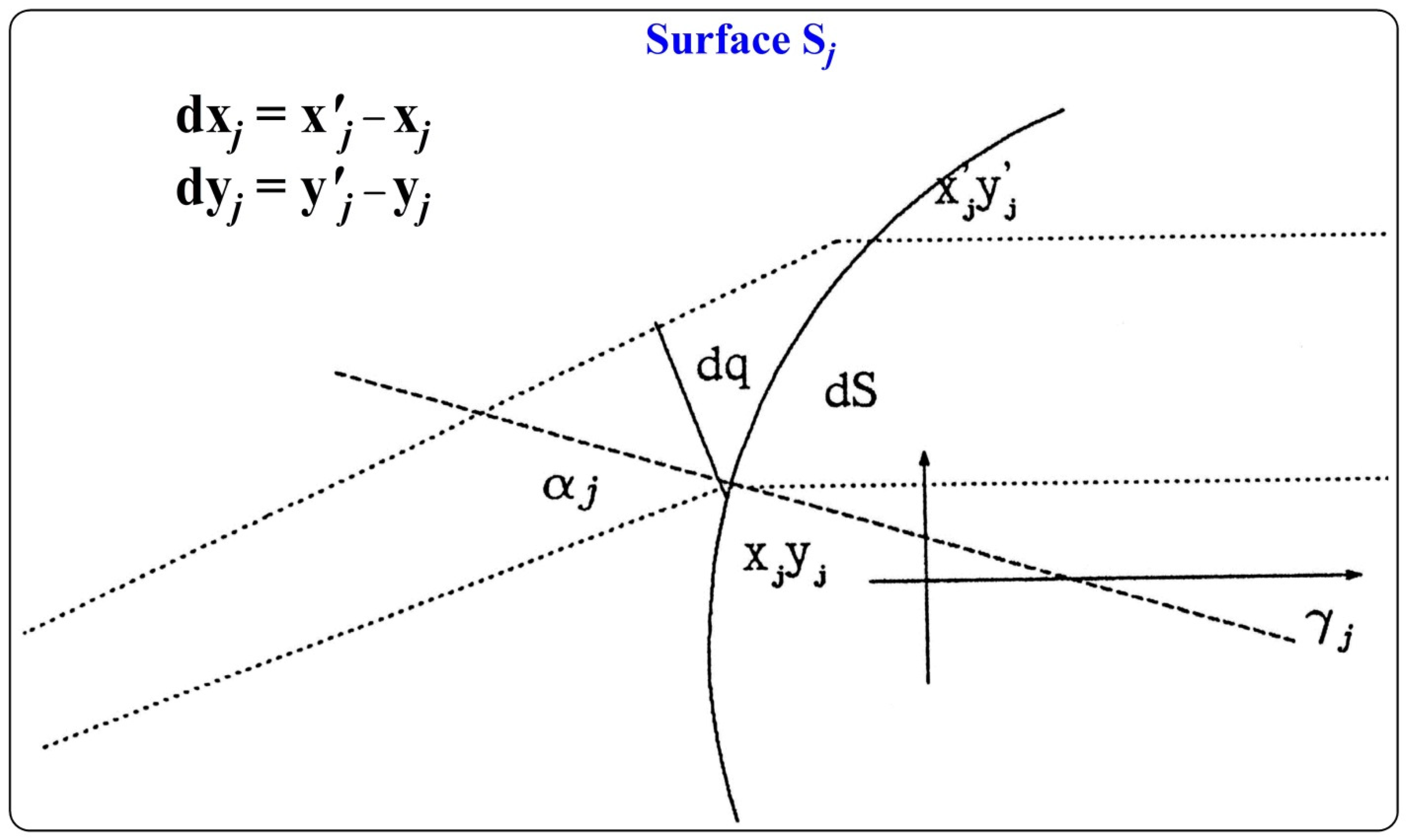
where x, y are the coordinates of the ray, β is the ray direction angle, β_j is the angle of the ray at the point of reflection (or refraction) from the optical surface S_j (Figure 1), t is the time, v is the seismic velocity, Δl is the length of the ray, and j is the optical element.

The refraction or reflection angles of the ray could be calculated using Snell’s law [3]. After introducing j as the angle of normal to the surface S_j, one can write:

(a)

for refraction:

$$1/v_j\sin \left({\gamma }_j-{\beta }_j\right)=1/v_{j-1}\sin \left({\gamma }_j-{\beta }_{j-1}\right),$$

(4)

(b)

for reflection:

$${\beta }_j=2{\beta }_{j-1}-\frac{\pi }{2}-{\gamma }_j.$$

(5)

The constant velocity of optical elements makes it possible to simplify the equation of dynamic ray tracing [16]:

$$\frac{dQ}{dl}=vP,\hspace{1em}\hspace{1em}\frac{dP}{dl}=\frac{1}{v^2}\frac{{\partial }^{2}v}{\partial q^2}Q,$$

(6)

where Q is the spreading function, P is the derivative of the slowness in a direction tangent to the wavefronts, v is the seismic velocity, l is the ray’s length, and q is the distance on the normal to the ray.

For the case of a conventional optical model, an equation of dynamic ray tracing may be presented in the following form [17]:

$$Q_{j-1}=v{P}_j\mathsf{\Delta }l, P_j=\mathrm{const}.$$

(7)

Examining the behavior of the paraxial rays, one can see that the angle between two rays will stay constant during the propagation in the model with constant velocity. This angle will change only after reflection or refraction. For a case of linear approximation, one has:

$$\mathsf{\Delta }\beta =vP\mathsf{\Delta }\mathit{\Theta }\mathrm{o} ,$$

(8)

$$\mathsf{\Delta }\mathit{q}=\mathit{Q}\mathsf{\Delta }\mathit{\Theta }\mathrm{o} ,$$

(9)

where ΔΘ_o is the angle between two initial incident rays: central and paraxial (see also Figure 4), the elements Δβ and Δq are the angle and the distance between the central and paraxial rays inside optical system, respectively, when the ray ridge is the same wavefront (see Figure 1). For numerical calculation, the following expressions can be used.

(a)

Case of refraction

$${}_{}{}^{\tau }Q{}_i{\cos \mathsf{\alpha }}_j^{\tau }=-{}_{}{}^{i}Q{}_i\cos {\alpha }_j^i,$$

(10)

$${}^{\tau }{P}_i{\cos }_j^i=-{}_{}{}^{i}P{}_i{\cos }_j^i-\left({\frac{1}{\mathrm{v}}}_{j-1}\cos {\alpha }_j^r-{\frac{1}{\mathrm{v}}}_j\cos {\alpha }_j^i\right)\frac{{}_{}{}^{i}Q{}_i}{R_s},$$

(11)

where τ is the altering of the value after refraction; Q_j is the index of the incident wave, j is the number of layers, ${\alpha }_j^i={\beta }_{j-1}-{\gamma }_j$ is the angle between the incident and normal rays to the surface S_j, ${\alpha }_j^r={\beta }_j-{\gamma }_j$ is the angle between the refracted ray and the normal to the same surface. R_s is the radius of curvature to the surface in the point of refraction (the value is positive if the incident ray met the surface).

(b)

Case of reflection

Let us assume: ${\alpha }_j^i={\alpha }_j^r$ − π/2. Then

$${}_{}{}^{k}Q{}_j={}_{}{}^{i}Q{}_j,$$

(12)

$${}^k{P}_j={}_{}{}^{r}P{}_i-\left({\frac{1}{v}}_{j-1}+{\frac{1}{v}}_j\right)\frac{{}_{}{}^{i}Q{}_j}{R_s},$$

(13)

where k is the index of the reflected wave.

Expression (6) is a linear differential equation with two independent solutions. Any other solution can be established as a linear combination of the obtained solutions.

Thus, one can write

$$\begin{array}{l}Q=a{Q}_1+b{Q}_2\\ P=a{P}_1+b{P}_2\end{array}\},$$

(14)

where a and b are the coefficients (the coefficients are introduced from the initial data of entered wavefront), and Q₁, P₁, and Q₂, P₂ are two independent solutions, respectively.

A radius of the wavefront curvature could be calculated as

$$R=\frac{Q}{vP}=\frac{a{Q}_1+b{Q}_2}{v\left(a{P}_1+b{P}_2\right)}.$$

(15)

Therefore, two independent solutions permit finding any wavefront curvature using these two fundamental solutions [36].

Equation (14) (or (6)) is a linear system of differential equations where only two equations are independent ones. Considering that Wronskian (determinant) is invariant, one obtains three independent solutions only (Q₁, Q₂, and P₂).

6. The Boundary Conditions

The accurate description of boundary conditions is highly significant for the precise optical system calculation. These conditions are usually formulated as incident and output wavefronts. The boundary conditions could be presented in the two following ways.

(a)

Boundary conditions are given for coordinates and angles of arrival and incidence rays. Together with the time of arrival, these conditions are necessary for the solution of an optical design system. Such methods are widely applied in the majority of known optical design software (e.g., [6,11,12,37]).

(b)

The second method is proposed in this investigation. The required boundary conditions are the wavefront curvature and distribution of the spreading functions of incident and arrival wavefronts [38,39].

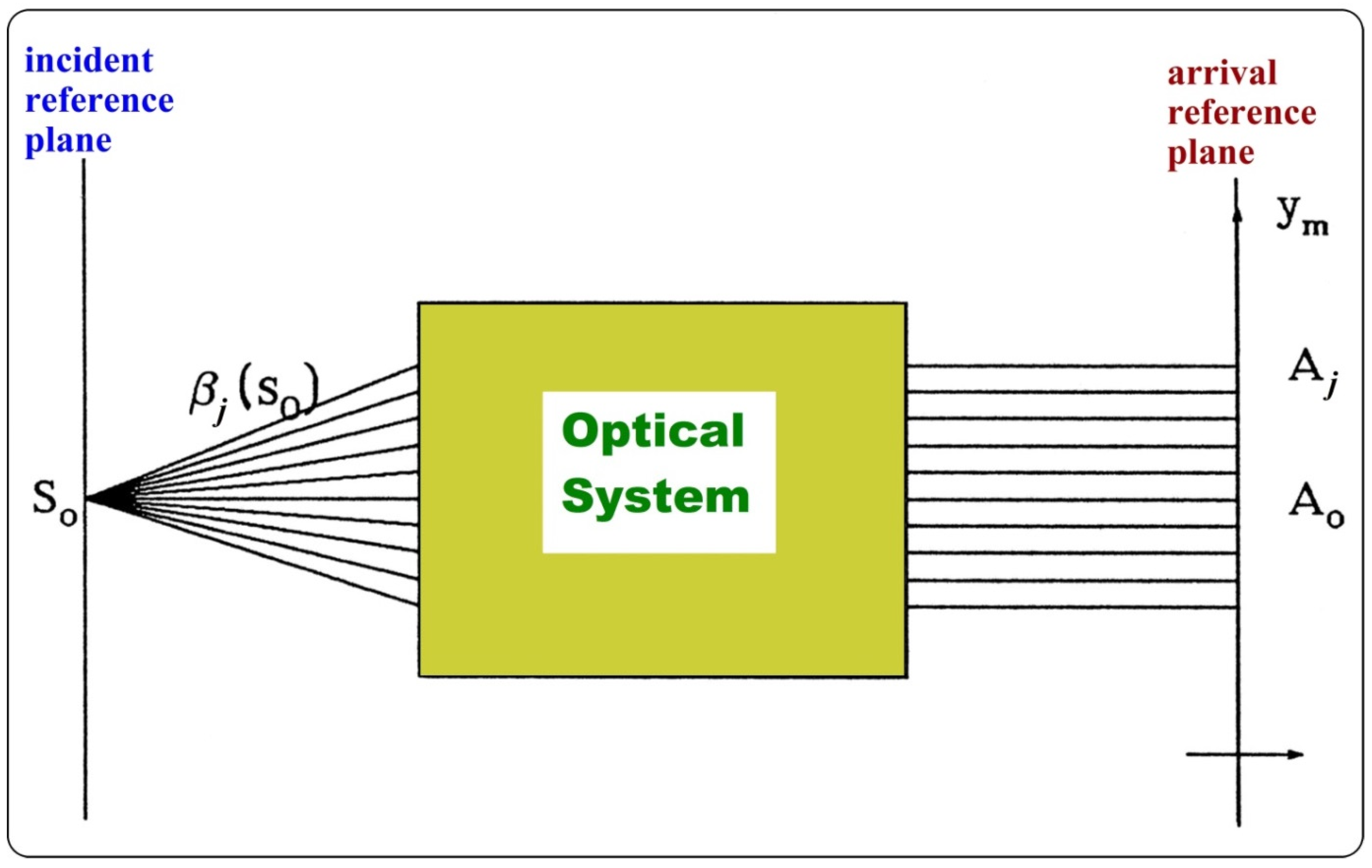
For example, in Figure 2 an optical system is presented, creating the plane wavefront with the constant distribution of the brightness as an output from undirected point of source S_o.

For each j-ray emitting from point S_o, one has the following initial conditions:

$$P\left(S_o\right)=1, Q\left(S_o\right)=0, R\left(S_o\right)=\frac{Q\left(S_o\right)}{P\left(S_o\right)V\left(S_o\right)}=0.$$

(16)

Respectively, output conditions for a plane front and constant brightness are the following:

$$P\left(A_j\right)=0, Q\left(A_j\right)=\mathrm{const}, R\left(A_j\right)=\frac{Q\left(A_j\right)}{P\left(A_j\right)V\left(A_j\right)}=\infty ,$$

(17)

where A_j is the point of j-ray that passed to the reference plane.

Taking into account that $Q\left(A_i\right)=\raisebox{1ex}{$\partial y$}\!\left/ \!\raisebox{-1ex}{$\partial {\beta }_i\left(S_0\right)$}\right.=const,$ the outside wave’s brightness distribution is also a constant value.

An example of such an optical system (for the described boundary conditions) is a telescopic objective with a focal length defined according to the definition [3]:

$$F=\frac{Q\left(A_0\right)}{P\left(S_0\right)}=const.$$

(18)

Another application of these boundary conditions is an optical system calculation where the Gaussian plane beam of a laser is reconstructed to the plane wave with the constant distribution of brightness along the wavefront (Figure 3).

One can assume that the function f(y) represents the brightness of the laser source. The boundary conditions can be written in such a way:

for incident plane,

$$P\left(S_j\right)=0, Q\left(S_i\right)=f\left(y_i\right),$$

(19)

for arrival plane,

$$P\left(A_j\right)=0, Q\left(A_i\right)=1.$$

(20)

The boundary conditions can include two or more wavefronts (geometrical modes).

7. The System of Differential Equations for Computing the Optical System

Based on the boundary conditions and employing the non-linear optimization (in such a way that modes with initial conditions will arrive with chosen conditions), it is possible to find the radius of curvature of the surface at the point of the ray intersection (refraction or reflection) with the surfaces. The number of the boundary conditions (number of the geometrical modes) gives the number of necessary unknown surface curvatures. However, when the number of surfaces is more significant than the number of boundary conditions of the calculated system, part of the curvatures in the system should be given earlier.

The selected ray satisfying the necessary conditions gives knowledge of the values Q_j and P_j at the points of intersection. These values make it possible to write the differential equations for coordinates of the points of paraxial ray intersection with the same surfaces (Figure 4).

$$\mathsf{\Delta }q=Q_j{\mathsf{\Delta }}_0\theta , \mathsf{\Delta }S=\frac{\mathsf{\Delta }q}{\cos {\alpha }_j}=\frac{Q_j\mathsf{\Delta }{\theta }_0}{\cos {\alpha }_j}.$$

(21)

Taking into account that $\partial x=\partial S\cos {\gamma }_i, \partial y=\partial S\sin {\gamma }_j$, one can write the differential equation of the surfaces

$$\begin{array}{c}\frac{\partial x_j}{\partial {\theta }_0}=\frac{Q_j}{\cos {\alpha }_j}\cos {\gamma }_j\\ \frac{\partial y_j}{\partial {\theta }_0}=\frac{Q_j}{\cos {\alpha }_j}\sin {\gamma }_j\\ \left(j=1,2,\dots ,m-1\right)\end{array}\}.$$

(22)

System (22) is the linear homogeneous equation system where each term can be calculated numerically in satisfaction with the boundary conditions. Two differential equations represent each surface. Thus, a system of 2(m − 1) equations could be used to construct the whole optical instrument.

For the optical systems with diffractive elements, Equation (20) describes the piecewise smooth surfaces; when on the singular points, the changing of coordinates which are moved on a length of the wave should be simultaneously introduced.

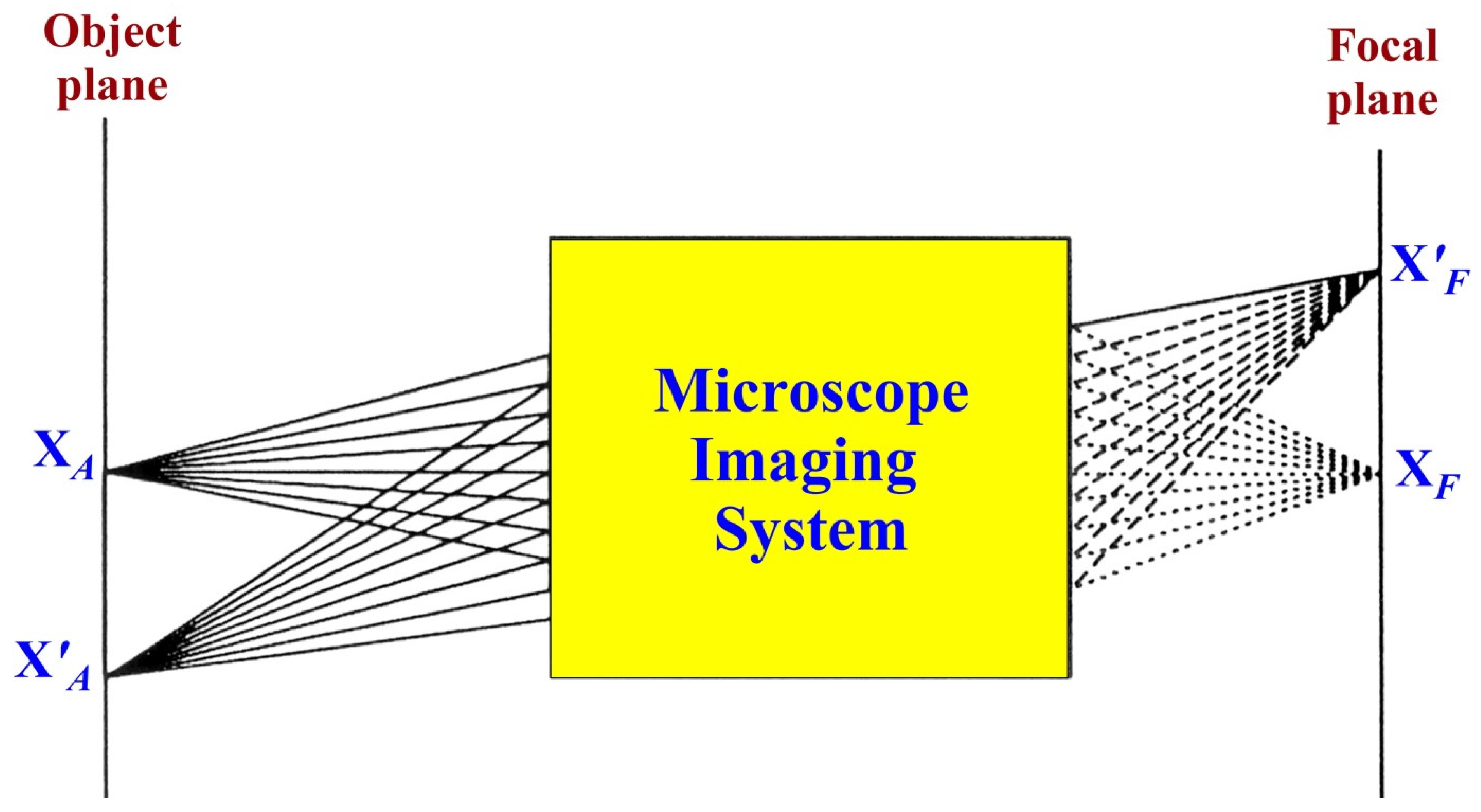
8. Boundary Conditions for an Ideal Imaging System

An ideal microscope is an imaging system applying for close examination of various small targets. In the ideal microscopic imaging system, the rays propagating from one point of an object should coincide at one point on the focal plane (Figure 5). However, in reality, the geometric rays in any optic system are distributed in some areas around this point. At the same time, rays from different object points do not coincide and will be distributed according to the angles of their entry. This phenomenon is known as an aberration. For the axisymmetric systems, the problem of coma aberration reduction is most challenging.

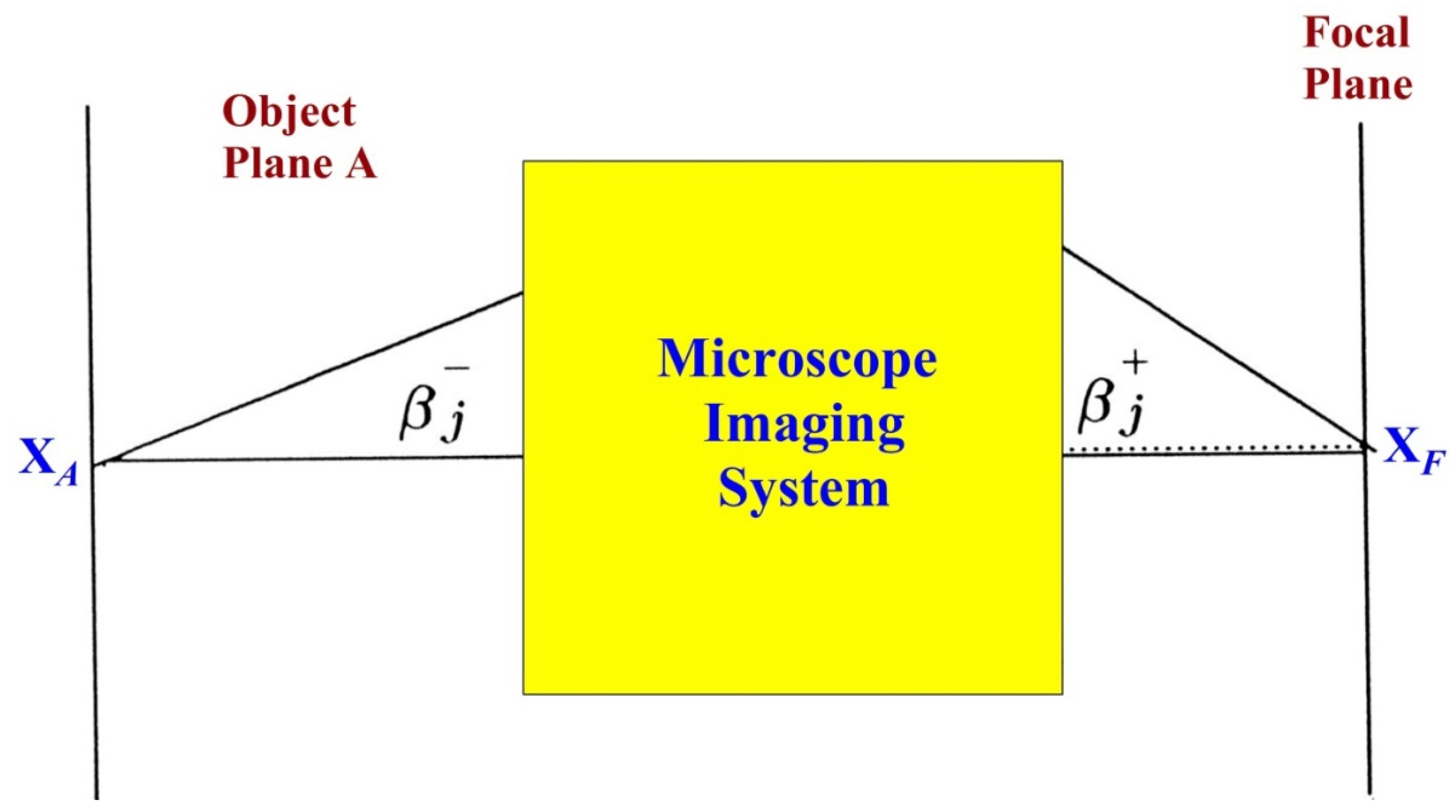
8.1. Boundary Conditions for a Microscope System without Spherical Aberration

For a system without spherical aberration, the rays emitted from point x_A will be gathered at the point x_F. Each ray “j” of a fan emitted from point x_A in a direction enters the point x_F with the angle. Index “j” will designate propagation along the ray j. For a perfect optical imaging system on each ray, two fundamental wavefronts must correspond to the definite boundary conditions. The first boundary condition corresponds to removing spherical aberrations, while the second is removing coma aberration. The boundary conditions for a microscope system without spherical aberration can be written as:

(a)

emitted from point x_A on plane A (Figure 6) before the system:

$$P_1^j\left(x_A\right)=1,Q_1^j\left(x_A\right)=0,$$

(23)

(b)

at the focal point F at the surface Γ (where the rays are gathering together):

$$P_1^j\left(x_F\right)=C^j\left(x_F\right),Q_1^j\left(x_F\right)=0,$$

(24)

where $C^j\left(x_F\right)$ is an unknown function.

8.2. Boundary Conditions for a Microscope System without Coma Aberration

The boundary conditions for the case when rays emitting from the point X_A’ are gathering together at the point $x_F^{\prime }$ are more complex.

8.3. Determination

The conditions for the microscope optic system without coma aberration are the following: the plane wavefront propagated from the point $x_A^j$ along the ray j will be focused on the bold part of the sphere (Figure 7), and the second (thin) part of the sphere will be a focal surface of the system.

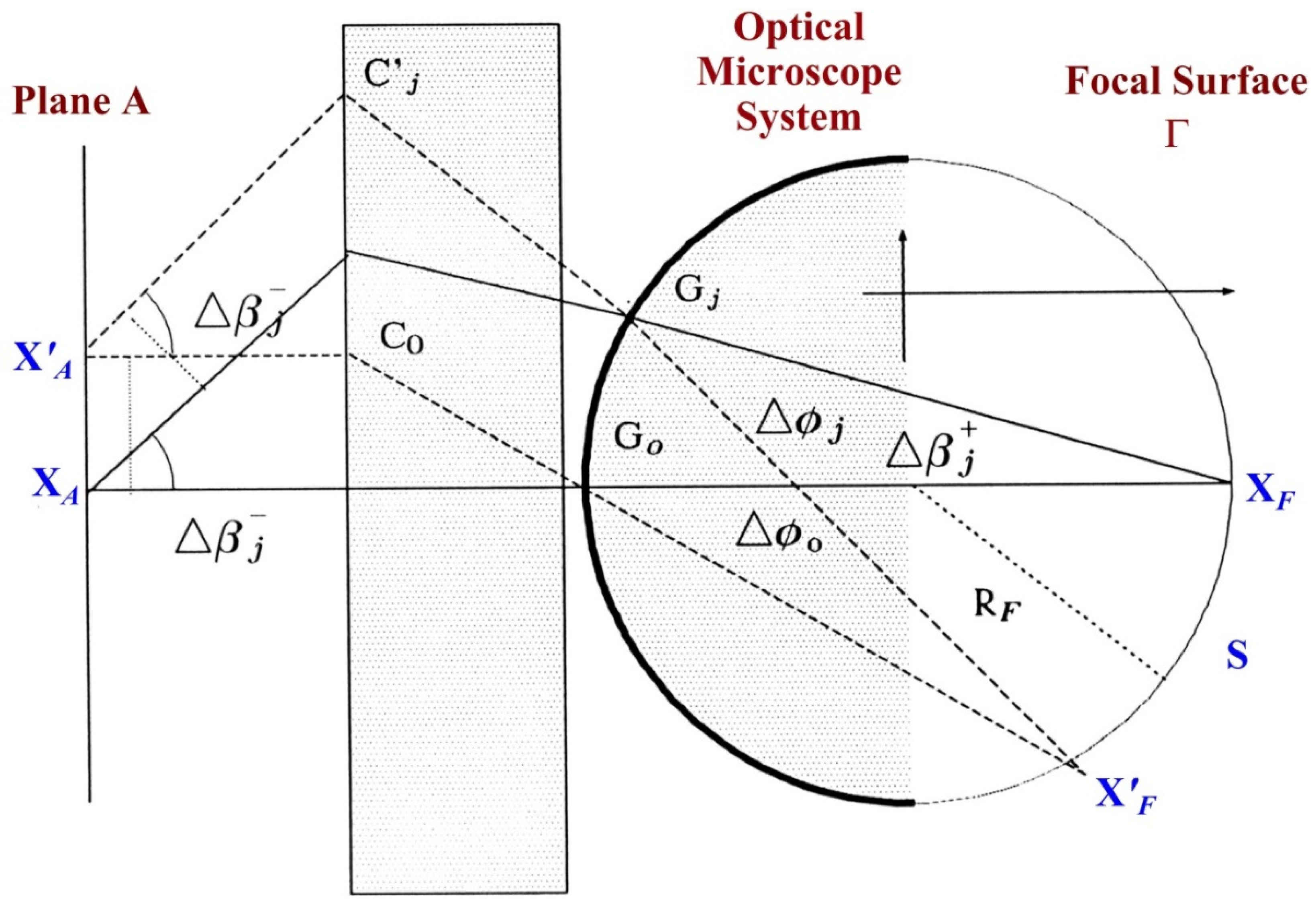
8.4. Explanation

Let us observe two rays emitted from the point $x_A^{\prime }$. The first ray (x_A, $c_o^{\prime }$) is emitting parallel to the optic axis (β = 0), and the second ray (x_A, $c_j^{\prime }$) is emitting from the point $x_A^{\prime }$ parallel to the ray emitted from point x_A with the angle β_j (see Figure 7).

Two pairs of parallel rays create two plane wavefronts propagated: first—along the optic axis; second—along the ray j. According to the mentioned conditions, these wavefronts will be focused on the points G₀ and G_j on the sphere R_F. In the ideal system, all rays emitted from the points $x_A^{\prime }$ and x_A are gathered together at the points $x_F^{\prime }$ and $x_F$ (see Figure 7).

Two angles that are at the same segment of the arc S (see Figure 7), taking into account known geometric theorems, have the same values:

$$\angle x_F{G}_j{x}_F^{\prime }=\angle x_F{G}_0{x}_F^{\prime }=\Delta \psi =\Delta {\psi }_j=\Delta {\psi }_0.$$

(25)

Let us assume a radius R_F of the sphere. The rays emitted from point source $x_A^j$ at the plane A with any j, and paraxial rays emitted with any angle θ from this point, are gathering together at the one point $x_j^{F\prime }$ only at the focal surface. It is obvious that the wavefront of the point source emitted from plane A will focus on the dash part of the sphere (point G_j). Then, all rays entering the system with the same angle will gather together at one point $x_j^{F\prime }$ (on the right part of a considered sphere in Figure 7).

The boundary conditions for the rays emitted from point x_A and arrived in the point x_F (responsible for the absence of coma aberration) could be written in the following manner. Let us assume a fictitious point source G_j that emits two rays in different directions along with the rays j: first one—to the focal surface; the second one—to the object.

For a direction to the focal surface, the length of the arc is

$$S=Q_2^{+}\left(C_j{x}_F\right)\Delta \psi .$$

(26)

It is important that the length S will be a constant value for all rays j. Therefore,

$$Q_2^{+}\left(C_j{x}_F\right)=Q_2^{+}\left(C_j{x}_F\right)\cos {\beta }_j^{+}=2R_F\cos {\beta }_j^{+},$$

(27)

$$P_2^{+}\left(C_j{x}_F\right)=P_2^{+}\left(C_0{x}_F\right)=1,$$

(28)

where R_F is the radius of the local surface.

We introduce that the wavefronts propagate in the media with a constant velocity. The conditions for the wavefront, propagating from the point source G_j to the plane of the object, are the following [39]:

a length of the object:

$$\Delta x^{-}=Q_2^{-}\left(C_0{x}_A\right)\Delta \psi =\frac{Q_2^{-}\left(C_j{x}_A\right)\Delta \psi }{\cos {\beta }_j^{-}},$$

(29)

where $Q_2^{-}\left(G_0{x}_A\right)=f$ (a local length of the optical system) and $\Delta x^{-}$ should be equal for all rays and wavefronts arriving as the plane wavefronts.

As a result

$$Q_2^{-}\left(G_j{x}_A\right)=f\cos {\beta }_j^{-},$$

(30)

and

$$P_2^{-}\left(G_0{x}_A\right)=P_2^{-}\left(G_j{x}_A\right)=0.$$

(31)

After combining the conditions together, one can write the following equations for the ideal imaging microscope system:

on the plane,

$$P_1^j\left(x_A^j\right)=1,\hspace{1em}\hspace{1em}{Q}_1^j\left(x_A^j\right)=0,$$

(32)

$$P_2^j\left(x_A^j\right)=0,\hspace{1em}\hspace{1em}{Q}_2^j\left(x_A^j\right)=f\cos {\beta }_j^{-},$$

(33)

and at the point x_F on the local surface,

$$P_1^j\left(x_F\right)=C^j\left(x_F^{}\right),\hspace{1em}\hspace{1em}{Q}_1^j\left(x_F\right)=0,$$

(34)

$$P_2^j\left(x_F\right)=1,\hspace{1em}\hspace{1em}{Q}_2^j\left(x_F\right)=2R\cos {\beta }_j^{+},$$

(35)

Here, function C(x_F) could be easily estimated, considering the Wronskian invariance:

$$C^j\left(x_F\right)=\frac{f\cos {\beta }_j^{-}}{2R_F\cos {\beta }_j^{+}}.$$

(36)

Then, the conditions considered may be written in the form:

on the plane

$$P_1^j\left(x_A\right)=1,\hspace{1em}\hspace{1em}{Q}_1^j\left(x_A\right)=0,$$

(37)

$$P_2^j\left(x_A\right)=0,\hspace{1em}\hspace{1em}{Q}_2^j\left(x_A\right)=1,$$

(38)

at the point x_F on the local surface

$$P_1^j\left(x_F\right)=\frac{f\cos {\beta }_j^{-}}{2R_F\cos {\beta }_j^{+}},\hspace{1em}\hspace{1em}{Q}_1^j\left(x_F\right)=0,$$

(39)

$$P_2^j\left(x_F\right)=1,\hspace{1em}\hspace{1em}{Q}_2^i\left(x_F\right)=\frac{2R\cos {\beta }_j^{+}}{f\cos {\beta }_j^{-}}.$$

(40)

The presented investigation is a basis for developing a new theory of design and calculation of diffracted and integrated optics systems and arrays. The authors suggest that the theory will be practical for computing optical systems consisting of many (demanding) numbers of optical elements of complicated (arbitrary) shapes. The essential benefit of the developed procedure compared with other known methods is the simultaneous calculation of the unlimited number of optical surfaces with different shapes (spherical, aspheric, diffractive, and the mixing of complex combinations of these surfaces) with complicated contours and required accuracy.

The suggested method could be generally used in non-conventional optics: analysis, design, and employment of optical systems and arrays consisting of diffractive microlenses, elements of spherical and aspherical surfaces, and hybrid elements.

9. Conclusions

It is shown that there is an analogy between the inversion of registered wavefields in seismic prospecting and the development of optical systems design. The procedure “homeomorphic imaging”, developed in seismic prospecting, could be effectively applied to calculate complex optical systems with arbitrary shapes, large apertures, and arbitrary angles of incidence. With the goal of detailed descriptions of complex optical systems, novel boundary conditions based on the employment of dynamic ray tracing developed in seismic prospecting are proposed for use. For various optical systems (telescope, microscope, etc.), specific boundary conditions should be developed (illustrated in the example of a microscope system). These boundary conditions and respective differential equations make it possible to create a more concise description of complex optical systems and compute their optical surfaces more accurately. In addition, it is essential for the calculation of complex aspherical surfaces and for creating a reliable infrared methodology of observations. Finally, the feasibility of the proposed approach application is displayed in examples of microscope imaging and afocal systems.