Abstract
The present paper reports on the methods of the systematic analysis of the high-energy collision distributions—in particular, those adopted by Jean Cleymans. The analysis of data on high-energy collisions, using non-extensive statistics, represents an important part of Jean Cleymans scientific activity in the last decade. The methods of analysis, developed and employed by Cleymans, are discussed and compared with other similar methods. As an example, analyses of a set of the data of proton-proton collisions at the center-of-mass energies, and 7 TeV, are provided applying different methods and the results obtained are discussed. This line of research has the potential to enlarge our understanding of strongly interacting systems and to be continued in the future.
1. Introduction
One of the most evident features of high-energy collision (HEC) experimental data is the observation of the q-exponential distributions of the energy and momentum of the created particles. The experimental evidence motivated many studies on the use of Tsallis statistics in the multiparticle production process [1]. The role played by Jean Cleymans in the efforts to clarify the non-extensive aspects of the HEC can hardly be overestimated. He was a leading researcher on the Hadron Resonance Gas model [2,3] approach to the high-energy phenomena, and soon assumed a fundamental role in the investigations of the non-extensive generalization of the model using the Tsallis statistics [4].
One of Cleymans’ best-known contributions to the study of the non-extensive distributions presents the formula for the distribution, derived from the non-additive entropy by using the thermodynamical relations [5]. With this formula, Cleymans performed a series of studies with several collaborators, developing systematic analyses of the experimental data and finding important patterns in the behavior of the parameters of the formula [6,7,8,9]. The investigations on the physical meaning of the non-extensive statistics involved systematic research for different energies and different particle multiplicities [7,10,11]. Cleymans was also involved in predictions of the outcomes for future experiments; the latter were largely confirmed by the experimental data.
One fundamental contribution to the investigation of the hadronization of the quark–gluon plasma was the theoretical determination of the critical line for the confined–deconfined regimes of the hadronic matter [12]. This study was subsequently generalized to include the non-extensive statistics [13]. With this work, Cleymans opened the opportunity to apply the knowledge, gathered in HEC, to other fields, such as neutron–star modeling. This illustrates the importance and the reach of Jean Cleymans’ work. In one of his last papers [6], Cleymans and his collaborators present an accurate analysis of the non-extensive distributions for a wide range of collision energies and for several particle species. The study includes a detailed analysis of the covariances of the fitting parameters, largely extending previous investigations. Such an accurate analysis is of relevance in view of the predictions, by a thermofractal model of quantum chromodynamics (QCD), that the value for the entropic parameter, q, is calculated in terms of the fundamental parameters of the theory, namely, the number of colors, , and the number of flavors, , by a famous relation, , resulting to [14]. Cleymans’ study represents a rigorous test for the theoretical prediction [9]. The line of research, to which Cleymans contributed so extensively, is believed to continue to develope for many years to come, contributing to our knowledge about the strongly interacting systems.
In this paper, a systematic analysis of the HEC data is conducted in the style that Cleymans used to perform in his late years. The formula by Cleymans for the transverse momentum () distribution is used to fit the experimental data at different energies and for different particle species. The results are compared with the fits, obtained by other formulas. The analysis, presented here, is restricted to proton-proton () collisions, since, for larger systems, other phenomena can interfere, such as the collective flow. The inclusion of this effect in the statistical description of the multiparticle production is possible, but it demands additional parameters, which we want to avoid at this stage of the investigation.
2. Momentum Distributions
The main formula for -distribution is
where N is the number of particles, V is the volume g, p, y, and denote the the particle degeneracy, momentum, rapidity, and chemical potential, respectively, and is the particle transverse mass, , with the remaining mass of the particle. Equation (1) was shown by Cleymans and Worku [5] to be a direct consequence of the Tsallis non-additive entropy when the correct thermodynamical relations are applied. In what follows, Equation (1) is addressed as the Cleymans formula.
All parameters in the Cleymans formula present well-understood physical meanings, and the insistence of Cleymans in the use of the correct formula shows that he always considered the Tsallis statistics to play an underlying physical role in the high-energy processes. Many studies, presenting analyses of HEC data using Cleymans’ approach, have appeared during the last few years [15,16,17,18,19,20,21,22,23].
It is typical, however, to find different forms of the same expression being used to fit high-energy collision distributions [24]. Setting and in Equation (1):
where the chemical potential is fixed to the particle mass, i.e., , and the power exponent, . However, the multiplication factor, , is absent in Equation (2), giving space to a dependence on the temperature, T. The term, , represents the rapidity density, and it is generally calculated in a small window around , being assumed to be an arbitrary constant in the fits. In what follows, Equation (2) is addressed as the Levy–Tsallis formula.
Another form of the distribution is the so called Tsallis–Pareto formula [25],
where C and are adjustable constants, which are obtained at and .
The three formulas are similar in many aspects, and they all fit the data well enough. The only important difference is the factor , which is changed into a temperature dependence normalization in Equation (2) and completely disappears in Equation (3). In short, in Equation (1) is changed to in Equation (2) and in Equation (3). To better understand the formulas and the approximations involved, it is constructive to calculate Equation (1) from the first principles, and then relate the result to other formulas; for a discussion about the behavior of the frequently used formulas, see Ref. [26].
The fundamental quantity is the number of one-particle configurations in the phase space according to Tsallis statistics, which is given by
where N is the number of particles per event, and p are the particle energy and four-momentum, respectively, with . Integrating over , and dividing by the total number of the particles produced in the event, one gets the probability density:
The rapidity y is defined by the relation,
where is the longitudinal momentum. From definition (6), . The independent coordinates of the momentum can be used to replace by y. The definition of the rapidity is equivalent to defining
therefore, and , where with v being the velocity of a beam in the rest frame and c the speed of light.
One can see that Equation (8) is similar to Equation (3) with and differs from Equation (1) by an absence of the multiplicative term . Equation (8) also differs from Equation (2), since the first equation has a dependence on the chemical potential that is not present in the second one. A detailed discussion about the Lorentz transformation of the transverse momentum distribution can be found in Ref. [18]. In what follows, Equation (8) is addressed as the Lorentz invariant cross-section formula.
In the analysis, a care should be taken the correct double differential distribution is used in terms of momentum components or in terms of rapidity, since this leads to different formulas. Moreover, the invariant differential distribution should be used. In the analysis below, the quality of the fits, obtained with the Formulas (1)–(3) and (8) is investigated, and the parameters obtained are compared in order to identify the correspondences. The non-extensive formulas, used here, are able to fit data of transverse momentum distributions over many orders of magnitude, and can be related to physical phenomena that need further investigation [1]. In the following, a brief discussion about the behavior of the parameters obtained with the different formulas is given, while a detailed consideration of the physical aspects of the results is left for the future.
3. Analysis
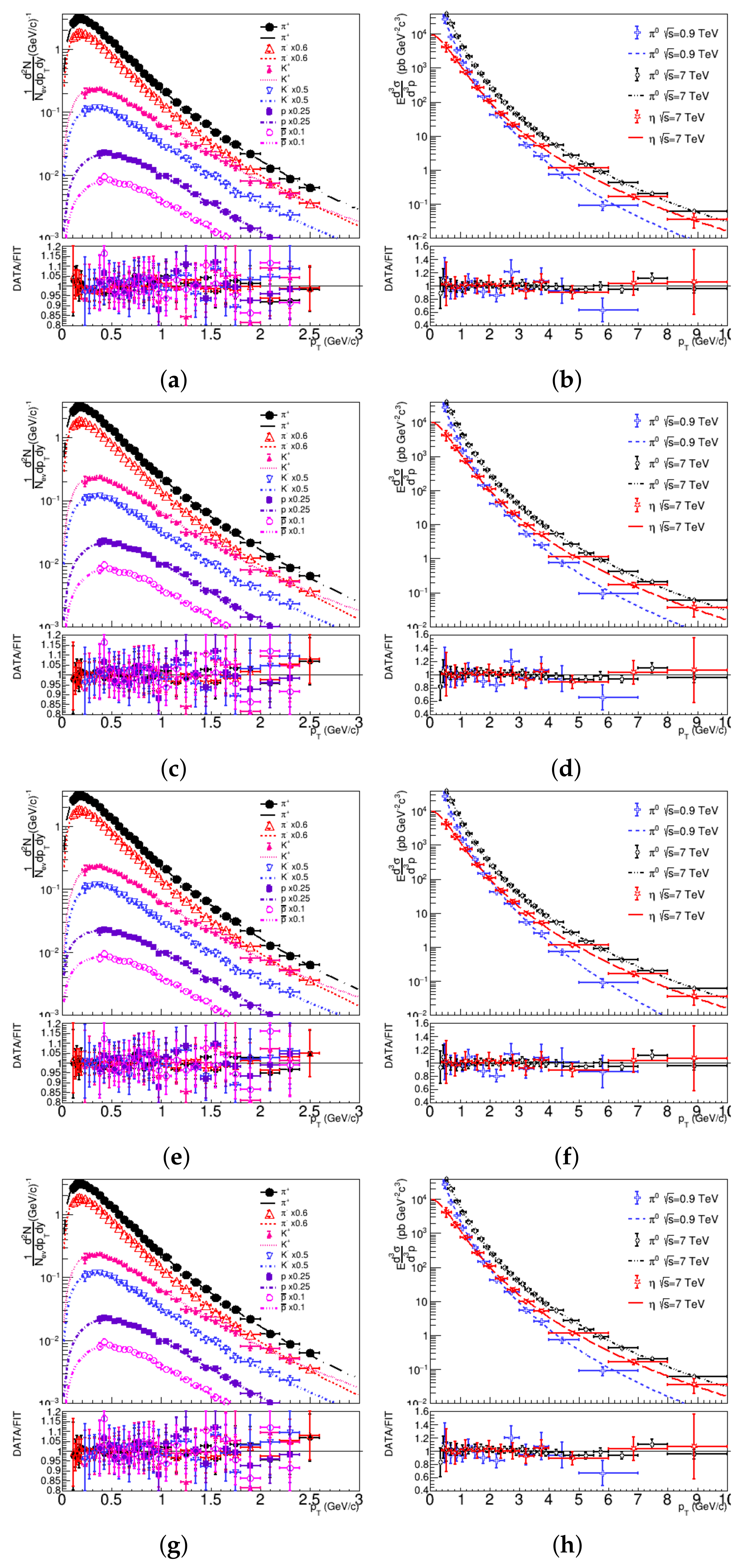
In the present analysis, the free parameters in Equations (1)–(3) are obtained by fits to the distributions from high-energy () collision data, reported in Refs. [27,28]. For Equation (3), two different methods are used for fitting the data distributions, namely, one using the parameter free to be adjusted to the measurements, and another method fixing : . The results of the fits for different particle species and energies, as fitted by each of the Formulas (1)–(3), analyzed here, are displayed in Figure 1. The best-fit parameters for each formula are displayed in Table 1, Table 2, Table 3, Table 4 and Table 5. Note that the errors of the multiplicative constant that result from the fits of the curves for the last three sets of data are much larger than the errors for the other cases.
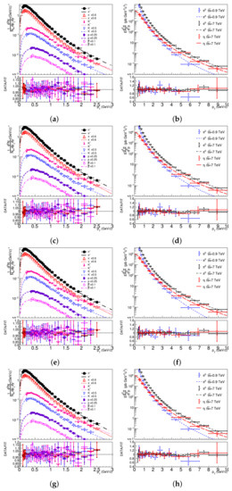
Figure 1.
The double-differential transverse momentum distributions with the fits by (a,b) Equation (1), (c,d) Equation (2), and (e–h) Equation (3), with the parameter left free (e,f) and (g,h). The data are from proton-proton collisons at the center-of-mass energies, 0.9 and 7 TeV; taken from [27,28].

Table 1.
Best-fit parameters of the Cleymans Formula (1). The data represent proton-proton collisions at the center-of-mass energies, and 7 TeV from Refs. [27,28]. The particle masses are taken from [29]. In the last column, the -statistics values are given per the number of degrees of freedom (ndf).


The large errors are due to the fact that, in these sets of data, the experimental data do not cover the region of the peak of the corresponding curves, as can be observed in the right panels of Figure 1. In these cases, the determination of the multiplicative constant, C, leads to a large number of combinations of T and C that can fit the data. The fitting procedure was performed with the use of the ROOT package, and the covariance matrix was obtained by using the MIGRAD routine in this package.
As one can observe from the values of the best fits, shown in Table 1, Table 2, Table 3, Table 4 and Table 5, all formulas fit the data well enough, except the small differences in the parameterization. One could expect that Equations (2) and (3) with would give similar results because the only difference is the incorporation of the temperature, T, in an overall normalization constant, C. This expectation is indeed observed in the results of the fits in Table 2 and Table 4. Since T does not depend on , this difference would be of no significance for the fits using Formulas (2) and (3). On the contrary, the Cleymans–Worku Formula (1) does have an additional dependence in the multiplication factor through the term . The effects of the factors and on the distributions can be understood notifying that
which is approximately constant and equal to for . Therefore, only in the low range of transverse momentum, the additional factor, , is insignificant for the fits. The temperature, T, is well determined in the sets of data that cover the peak in the -distribution.
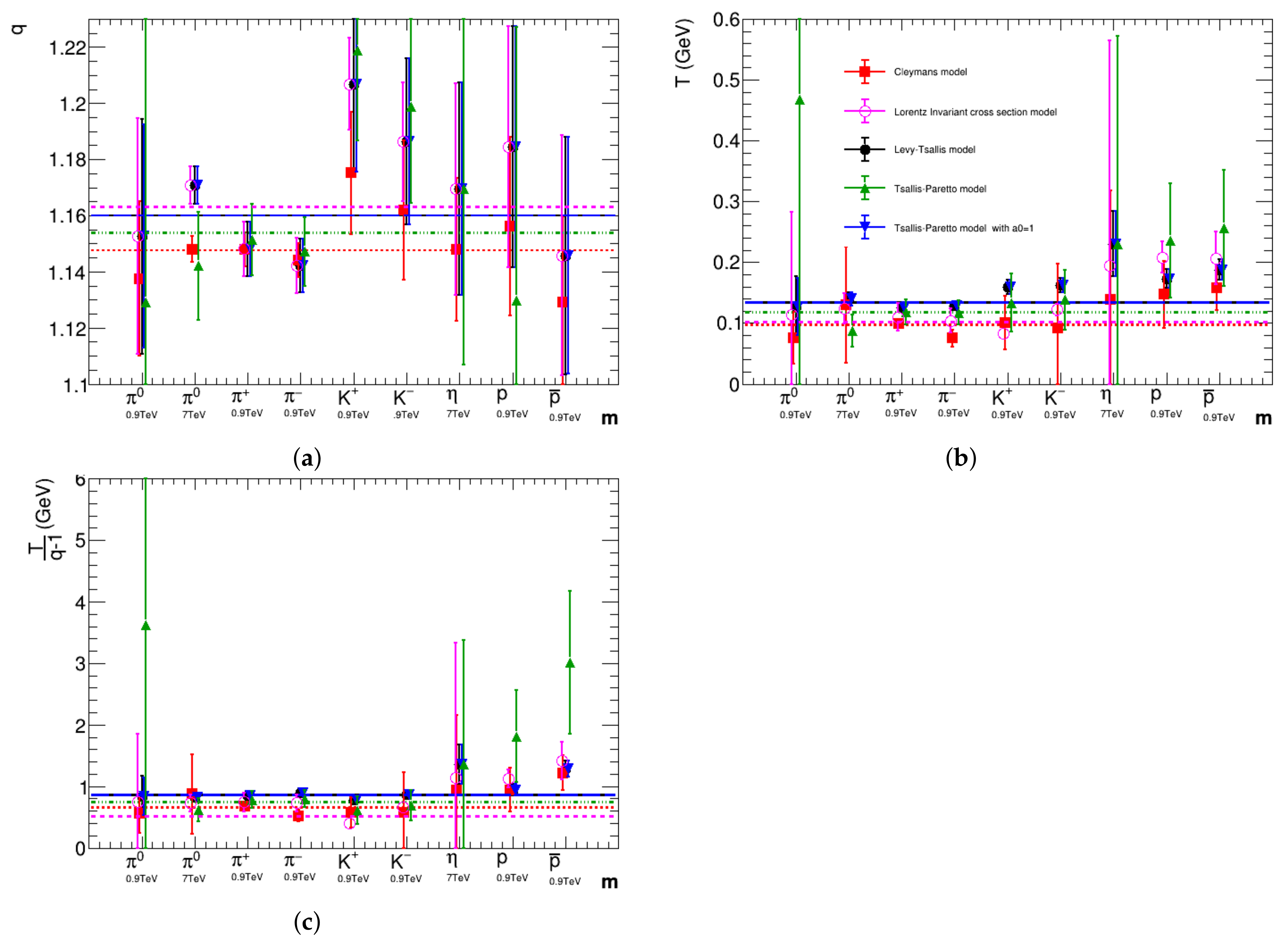
The systematic analysis of the parameters is performed by comparing the behavior of the parameters q and T, extracted from the fit. The relation between n and q is used where necessary. The results of the analysis of the mass dependencies of the parameters are displayed in Figure 2. One has to remember, that the different exponents in the Cleymans formula and in the other formulas will lead to different numerical values for q and T.

Figure 2.
Behavior of the Tsallis exponent, q, temperature, T, and the ratio, , as a function of the particle species. extracted from the fits with different formulas. The relation, , used where necessary (see the text for details). (a) Tsallis exponent, q (b) temperature, T (c) the ratio, .
Some authors, as in Refs. [1,18,25], adopt , and in such cases, it is possible to relate the values and from the Cleymans formula to the values and from the other formulas by the relations,
One observes that the results for the best-fit value of the parameter q are similar for all formulas used, with results fluctuating around the expected theoretical value of . Using the relation above, one may expect for the Cleymans formula. As can be observed in Figure 2a,b, there is no clear dependence observed on the particle mass or collision energy. The behavior of the parameter T, however, is different and shows a dependence on the particle mass for all formulas, except that for the Cleymans formula. This result might be related to the fact that, in the Cleymans formula, the chemical potential is a free parameter, while in the other formulas, it is the constant particle mass.
A theoretical study, generalizing Hagedorn’s self-consistent thermodynamics by the inclusion of the Tsallis statistics, leads to the non-extensive self-consistent thermodynamics [30], which predicts that the ratio should be independent of the the collision energy or particle species. In Figure 2c, this result is demonstrated by all formulas used, except the Tsallis–Pareto formula with the free parameter .
Contrary to what would be expected, the results of the analysis of the parameters show that the behavior of the parameters q and T is similar for Equations (1) and (2), but the values of the parameters differ from the values, obtained by Equation (3), mainly, for the heavier particles. Significantly smaller differences are observed from the comparison of the fits for other particles.
One can observe that, despite the plain curves, obtained with the formulas, used in the present analysis, the fitting procedure is not as direct. There are strong correlations among the fitting parameters, which can be observed by an analysis of the covariances. The introduction of the chemical potential as a free parameter makes the problem worse. Actually, it is always possible to obtain an equivalent fitting by fixing if the multiplicative constant and the temperature are both adjustable. This is an indication of the limits of an analysis, based exclusively on the -distribution data. Additional hypotheses or complementary analyses of, e.g., the ratio of the particle species yields, are necessary to determine unambiguously all the parameters.
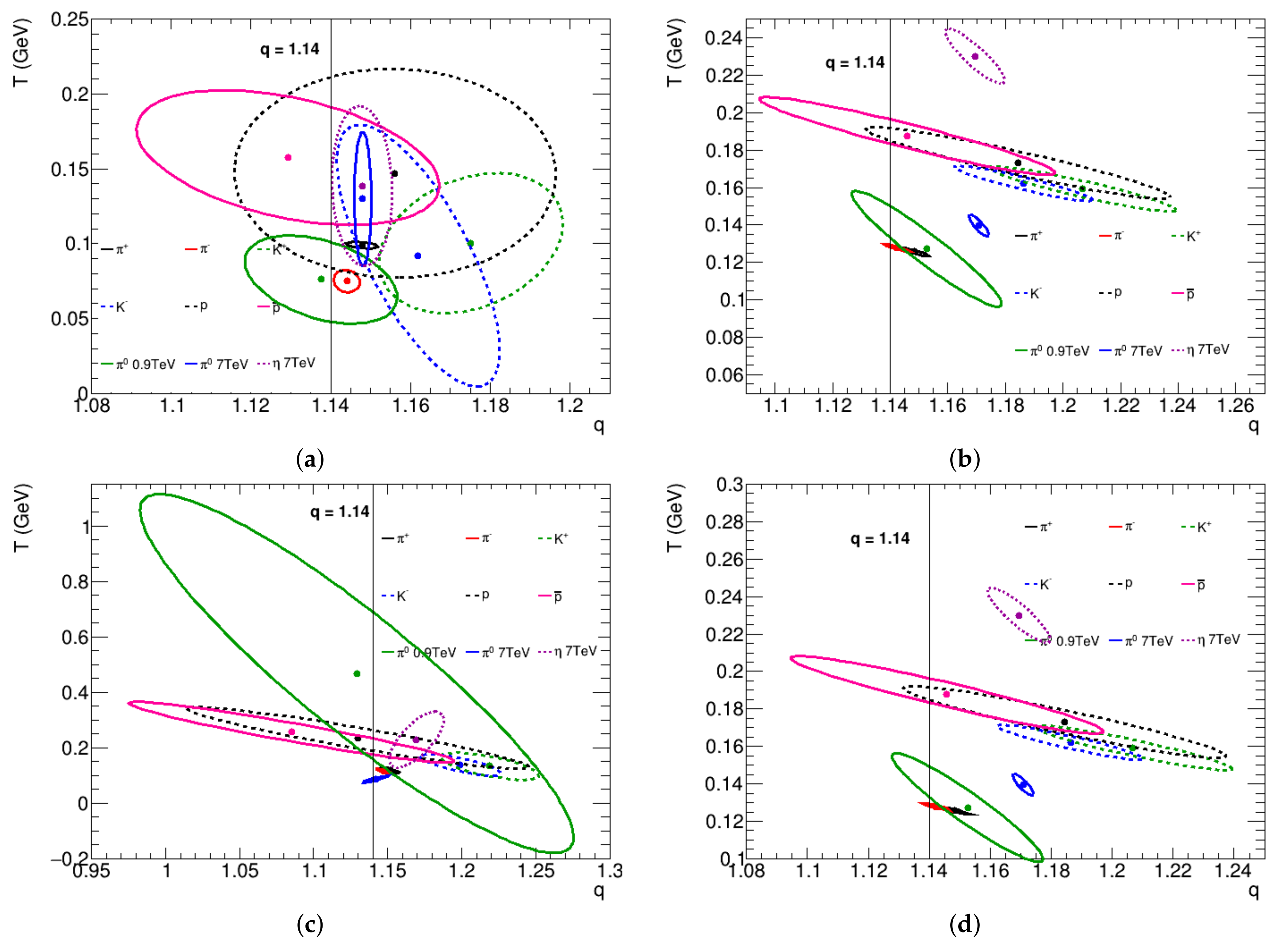
Whereas the differences in the formulas, used in this analysis, are subtle when observed through the obtained best-fit parameters, the analysis of the covariances among the parameters shows clear differences depending on the formula used. Figure 3 shows the correlation among the parameters q and T obtained for each particle species and collision energy and for all formulas, used in this analysis. The ellipses show the 5% confidence level of the fitting, demonstrating a strong correlation between these two parameters. The theoretical values are indicated in Figure 3 and one can see that the expected values are attained within errors for all formulas. One can also observe that the covariances change significantly from one formula to another, except of the Levy–Tsallis formula and the Tsallis–Pareto formula with . This was expected since these two formulas differ only by the inclusion of a multiplicative term that depends on q and T in the Levy–Tsallis formula.
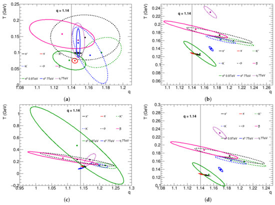
Figure 3.
Joint confidence region on the T–q plane in the parameter space, with significance, . The regions are obtained by using (a) Equation (1), (b) Equation (2), and (c,d) Equation (3), with (c) the parameter left free to adjust and (d) fixed to the value . The results for 7 TeV are indicated by the asterisks and the results for 0.9 TeV are indicated by the solid circles for the centers of the ellipses.
A final analysis is performed by using the Lorentz invariant cross-section Formula (8). Observe that the multiplication factor, , exponent, , and the chemical potential remains as an adjustable parameter. This formula allows us to test the hypothesis made above, i.e., that the variations in the temperature with the particle species, observed in some of the fits, are due to the fact that, in those cases, the chemical potential is fixed to the particle mass, while in the Cleymans formula, this parameter is an adjustable.
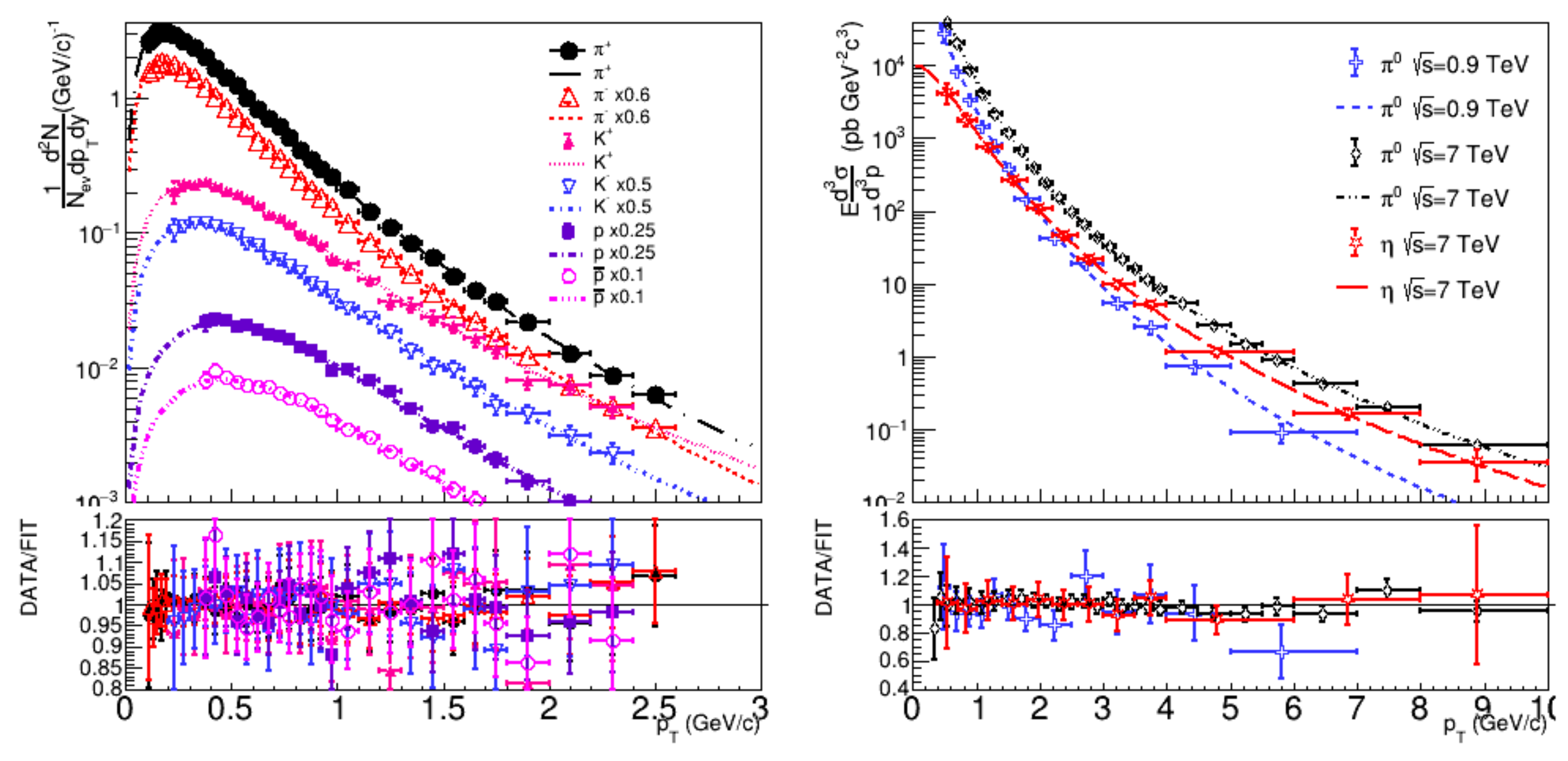
The results of the fittings with the Lorentz invariant cross-section formula are presented in Figure 4, and one observes that the data are well fitted also in this case. The best-fit parameters are listed in Table 5, and one can observe that the reduced , corresponding to the fitting, is small and comparable to those, obtained with other formulas.

Figure 4.
The double-differential transverse momentum distributions, fitted by the Lorentz invariant cross-section (8). The data are from [27,28].
The analysis of the parameters, obtained with the Lorentz invariant cross-section formula, are shown in Figure 2 by open circles. Whereas the results for q do not change significantly with respect to other formulas, one observes that the temperature, T, with the Lorentz invariant cross-section formula represents a behavior similar to that, observed with the Cleymans formula. Therefore, this result confirms the hypothesis that the dependence on T is due to the fact that the chemical potential is fixed in some of the formulas. The ratio, , remains almost constant, as observed in all other formulas with the multiplicative term proportional to .
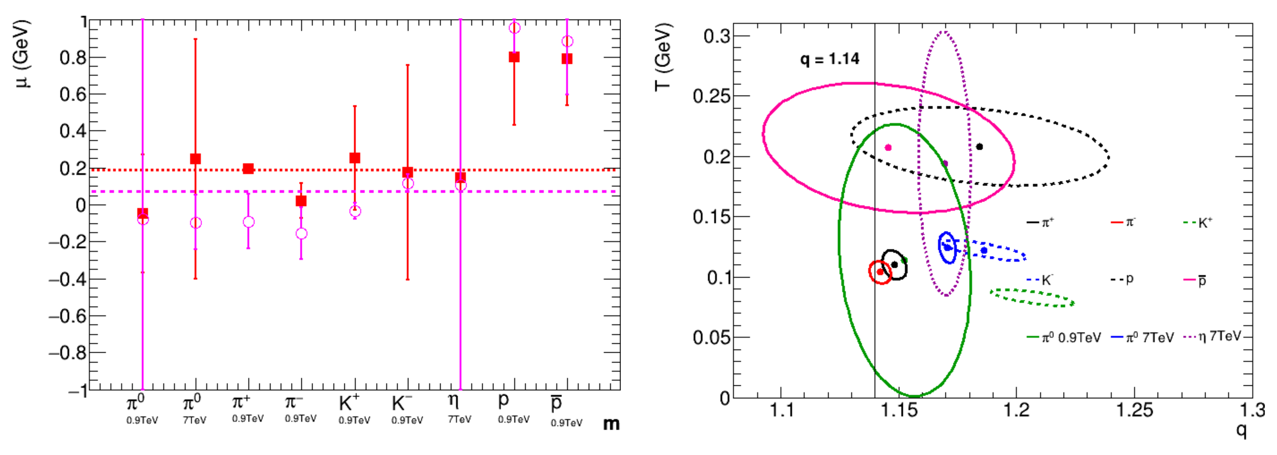
In Figure 5, the chemical potential is shown for different particle species and collision energies along with the covariances between the parameters T and q for the fit with the Lorentz invariant cross-section formula. One can see that the chemical potential does not present any evident dependence on the particle mass or on the collision energy, but may depend on the baryonic number, since it is slightly higher for the cases of the proton and the anti-proton. This is in contrast with the assumptions in the Pareto–Tsallis and Levy–Tsallis formulas, where the chemical potential is assumed to be equal to the particle mass.
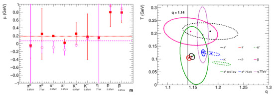
Figure 5.
Left: the dependence of the chemical potential, , on the particle species. The results are for the Cleymans Formula (1) (solid squares) and for the Lorentz invariant cross-section Formula (8) (open circles). The dotted and dashed lines represent the average value for the chemical potential, obtained by the Cleymans formula and the Lorentz invariant cross-section formula, respectively. Right: the covariances in the T–q plane in the parameter space, corresponding to Lorentz invariant cross-section Formula. The results for 7 TeV are indicated by the asterisks and the results for 0.9 TeV are indicated by the solid circles for the centers of the ellipses.
Except for proton and anti-proton, the chemical potentials are small or compatible with the value for all other particles, independently of the collision energy. This result is in agreement with the findings of Cleymans and collaborators [20], where it is shown that the correlations between the parameters T, , and the multiplicative constant, V, allow one to set and still obtain the same result with different values for T and V. Using the Lorentz invariant cross-section formula, it was verified that fixing leads to the same fitted curve, the best-fit value for q does not change, and the values for T and V change according to the relations, found in Ref. [20] for all particles species, analyzed in the present paper. Let us note that the ellipses showing the covariance of the parameters T and q, shown in Figure 5, are similar to those obtained for the Cleymans formula. This is an indication that the adjustable chemical potential parameter has an influence on the result for the parameter T, as discussed above, and, thus, interferes with the correlation between the fit results for T and q. To note also is that there is a shift in the centroid of the ellipses with respect to those of the Cleymans’ formula. This shift results from the different behavior of the multiplicative factor of the formulas with the transverse mass, .
4. Conclusions
In this paper, the analysis of the high-energy proton-proton collison data is performed using the methods of the non-extensive distributions developed by Jean Cleymans. The results are compared through different transverse momentum distribution formulas. It is shown that all formulas fit well the data, while giving different best-fit parameters.
The best-fit values of the parameters are discussed and, for the parameter q, the results are compared to the expected values according to the a fractal approach to quantum chromodynamics (QCD) [14]. In most cases, the predicted fractal approach value is attained by the different distributions; however, it is important to consider the covariances of the parameters, as shown in Figure 3 and Figure 5 (Right).
It is not the objective of this study to make definitive conclusions, based on the results obtained. A more comprehensive analysis to make firmer conclusions is needed and is planned for the future. However, the present paper illustrates the importance of this type of analysis, to great extent developed by Jean Cleymans, for the understanding of the complex phenomena taking place during the multiparticle production in high-energy collisions.
A new phenomenon has emerged [31] in the analysis of the particle distributions using the non-extensive statistics. Therefore, a correct and accurate description of the distributions, finding the hidden patterns in the obtained parameters, will allow us to advance further in the understanding of the QCD at the non-perturbative regime.
We would like to remark here that the present analysis needs to be continued by the inclusion of additional data sets in order to arrive at firmer conclusions. This will allow us to perform statistical tests for theoretical predictions. However, the procedure adopted here, analyzing exclusively the transverse momentum, , distributions, is not able to provide a complete determination of all the parameters. The point that any fit can be equally reproduced by fixing the chemical potential and allowing the temperature and the multiplicative factor to adjust freely is an indication that one needs additional hypotheses or complementary analyses of, e.g., the ratio of the yields of different particle species, in order to completely determine all parameters in the formulas. Nevertheless, one conclusion that can be drawn from this partial analysis is that a thermodynamical approach describes the multiparticle production process, and, therefore, the hypothesis of thermal equilibrium of the system at the freeze-out stage is robust.
Let us recall that in the non-extensive statistics, the temperature fluctuations play a major role, as has been demonstrated by many studies [24,32,33]. This aspect has implications in the equilibrium described by the Tsallis statistics, which must accommodate these fluctuations. This issue is considered in Ref. [34].
Author Contributions
All authors equally contributed to the present work. All authors have read and agreed to the published version of the manuscript.
Funding
The work of L.R. was supported by the Coordenação de Aperfeiçoamento de Pessoal de Nível Superior—Brasil (CAPES)—Finance Code 001, grant 88887.641069/2021-00, by Project PROEX. The work of A.D. was partially supported by the CNPq-Brazil, grant 304244/2018-0, by Project INCT-FNA Proc. No. 464 898/2014-5, and by FAPESP grant 2016/17612-7. The work of E.M. is supported by the project PID2020-114767GB-I00 financed by MCIN/AEI/10.13039/50110001103, by the FEDER/Junta de Andalucía-Consejería de Economía y Conocimiento 2014–2020 Operational Program under Grant A-FQM-178-UGR18, by Junta de Andalucía under Grant FQM-225, by the Consejería de Conocimiento, Investigación y Universidad of the Junta de Andalucía and European Regional Development Fund (ERDF) under Grant SOMM17/6105/UGR, and by the Ramón y Cajal Program of the Spanish MCIN under Grant RYC-2016-20678. The work of F.-H.L. was supported by the National Natural Science Foundation of China under Grant Nos. 12147215, 12047571, and 11575103, the Shanxi Provincial Natural Science Foundation under Grant Nos. 20210302124036 and 201901D111043, the Scientific and Technological Innovation Programs of Higher Education Institutions in Shanxi (STIP) under Grant No. 201802017, and the Fund for Shanxi “1331 Project” Key Subjects Construction. The work of K.K.O. was supported by the Ministry of Innovative Development of Uzbekistan within the framework of fundamental project No. F3-20200929146 on analysis of open data on proton-proton and heavy-ion collisions at the LHC.
Data Availability Statement
Not applicable.
Conflicts of Interest
The authors declare no conflict of interest.
References
- Wilk, G.; Włodarczyk, W. Quasi-power laws in multiparticle production processes. Chaos Solit. Fract. 2015, 81, 487–496. [Google Scholar] [CrossRef]
- Cleymans, J.; Hippolyte, B.; Paradza, M.W.; Sharma, N. Hadron resonance gas model and high multiplicities in p-p, p-Pb and Pb-Pb collisions at the LHC. Int. J. Mod. Phys. 2019, 28, 1940002. [Google Scholar] [CrossRef]
- Oeschler, H.; Cleymans, J.; Hippolyte, B.; Redlich, K.; Sharma, N. Ratios of strange hadrons to pions in collisions of large and small nuclei. Eur. Phys. J. 2017, 77, 584. [Google Scholar] [CrossRef][Green Version]
- Tsallis, C. Possible Generalization of the Boltzmann-Gibbs Statistics. J. Stat. Phys. 1988, 52, 479–487. [Google Scholar] [CrossRef]
- Cleymans, J.; Worku, D. The Tsallis distribution in proton-proton collisions at root s = 0.9 TeV at the LHC. J. Phys.-Nucl. Part. Phys. 2012, 39, 025006. [Google Scholar] [CrossRef]
- Cleymans, J.; Paradza, M.W. Tsallis statistics in high energy physics: Chemical and thermal freeze-outs. Physics 2020, 2, 654–664. [Google Scholar] [CrossRef]
- Rath, R.; Khuntia, A.; Sahoo, R.; Cleymans, J. Event multiplicity, transverse momentum and energy dependence of charged particle production, and system thermodynamics in pp collisions at the large hadron collider. J. Phys. G Nucl. Part. Phys. 2020, 47, 055111. [Google Scholar] [CrossRef]
- Khuntia, A.; Sharma, H.; Tiwari, S.K.; Sahoo, R.; Cleymans, J. Radial flow and differential freeze-out in proton-proton collisions at √s=7 TeV at the LHC. Eur. Phys. J. A 2019, 55, 3. [Google Scholar] [CrossRef]
- Bhattacharyya, T.; Cleymans, J.; Marques, L.; Mogliacci, S.; Paradza, M.W. On the precise determination of the Tsallis parameters in proton–proton collisions at LHC energies. J. Phys. G 2018, 45, 055001. [Google Scholar] [CrossRef]
- Cleymans, J.; Man Lo, P.; Redlich, K.; Sharma, N. Multiplicity dependence of (multi)strange baryons in the canonical ensemble with phase shift corrections. Phys. Rev. C 2021, 103, 014904. [Google Scholar] [CrossRef]
- Sharma, N.; Cleymans, J.; Hippolyte, B. Thermodynamic limit in high-multiplicity proton-proton collisions at √s=7 TeV. Adv. High Energy Phys. 2019, 2019, 5367349. [Google Scholar] [CrossRef]
- Bugaev, K.; Sagun, V.; Ivanytskyi, A.; Nikonov, E.; Cleymans, J.; Mishustin, I.; Zinovjev, G.; Bravina, L.V.; Zabrodin, E.E. Separate freeze-out of strange particles and the quark-hadron phase transition. EPJ Web Conf. 2018, 182, 02057. [Google Scholar] [CrossRef][Green Version]
- Azmi, M.D.; Bhattacharyya, T.; Cleymans, J.; Paradza, M. Energy density at kinetic freeze-out in Pb-Pb collisions at the LHC using the Tsallis distribution. J. Phys. G Nucl. Part. Phys. 2020, 47, 045001. [Google Scholar] [CrossRef]
- Deppman, A.; Megias, E.; Menezes, D.P. Fractals, nonextensive statistics, and QCD. Phys. Rev. 2020, 101, 034019. [Google Scholar] [CrossRef]
- Sena, I.; Deppman, A. Systematic analysis of p(T)-distributions in p plus p collisions. Eur. Phys. J. A 2013, 49, 17. [Google Scholar] [CrossRef]
- Liu, F.H.; Gao, Y.Q.; Li, B.C. Comparing two-Boltzmann distribution and Tsallis statistics of particle transverse momentums in collisions at LHC energies. Eur. Phys. J. A 2014, 50, 123. [Google Scholar] [CrossRef]
- Khandai, P.K.; Sett, P.; Shukla, P.; Singh, V. System size dependence of hadron pT spectra in p+p and Au+Au collisions at √sNN = 200 GeV. J. Phys. G Nucl. Part Phys. 2014, 41, 025105. [Google Scholar] [CrossRef]
- Wong, C.Y.; Wilk, G. Tsallis fits to pT spectra and multiple hard scattering in pp collisions at the LHC. Phys. Rev. D 2013, 87, 114007. [Google Scholar] [CrossRef]
- Marques, L.; Andrade, E.; Deppman, A. Nonextensivity of hadronic systems. Phys. Rev. D 2013, 87, 114022. [Google Scholar] [CrossRef]
- Cleymans, J.; Lykasov, G.I.; Parvan, A.S.; Sorin, A.S.; Teryaev, O.V.; Worku, D. Systematic properties of the Tsallis Distribution: Energy Dependence of Parameters in High-Energy p-p Collisions. Phys. Lett. B 2013, 723, 351–354. [Google Scholar] [CrossRef]
- Azmi, M.D.; Cleymans, J. Transverse momentum distributions in proton–proton collisions at LHC energies and tsallis thermodynamics. J. Phys. G Nucl. Part. Phys. 2014, 41, 065001. [Google Scholar] [CrossRef]
- Rybczynski, M.; Wlodarczyk, Z. Tsallis statistics approach to the transverse momentum distributions in p-p collisions. Eur. Phys. J. C 2014, 74, 2785. [Google Scholar] [CrossRef]
- Marques, L.; Cleymans, J.; Deppman, A. Description of high-energy pp collisions using Tsallis thermodynamics: Transverse momentum and rapidity distributions. Phys. Rev. D 2015, 91, 054025. [Google Scholar] [CrossRef]
- Bíró, G.; Barnaföldi, G.G.; Biró, T.S. Tsallis-thermometer: A QGP indicator for large and small collisional systems. J. Phys. G Nucl. Part. Phys. 2020, 47, 105002. [Google Scholar] [CrossRef]
- Shen, K.; Barnafoldi, G.G.; Biro, T.S. Hadronization within the non-extensive approach and the evolution of the parameters. Eur. Phys. J. A 2019, 55, 126. [Google Scholar]
- Zheng, H.; Zhu, L.; Bonasera, A. Systematic analysis of hadron spectra in p+p collisions using tsallis distributions. Phys. Rev. D 2015, 92, 074009. [Google Scholar] [CrossRef]
- ALICE Collaboration. Neutral pion and η meson production in proton–proton collisions at √s = 0.9 TeV and √s = 7 TeV. Phys. Lett. B 2012, 717, 162–172. [Google Scholar] [CrossRef]
- ALICE Collaboration. Production of pions, kaons and protons in pp collisions at √s = 900 GeV with ALICE at the LHC. Eur. Phys. J. C 2011, 71, 1655. [Google Scholar] [CrossRef]
- Griffiths, D.J. Introduction to Elementary Particles; John Wiley & Sons, Inc.: New York, NY, USA, 1987; Available online: http://nuclphys.sinp.msu.ru/books/b/Griffiths.pdf (accessed on 25 May 2022).
- Deppman, A. Self-consistency in non-extensive thermodynamics of highly excited hadronic states. Physica A 2012, 391, 6380–6385. [Google Scholar] [CrossRef]
- Wilk, G.; Włodarczyk, W. Some intriguing aspects of multiparticle production processes. Int. J. Mod. Phys. A 2018, 33, 1830008. [Google Scholar] [CrossRef]
- Wilk, G.; Wlodarczyk, Z. The imprints of nonextensive statistical mechanics in high-energy collisions. Chaos Solit. Fract. 2002, 13, 581–594. [Google Scholar] [CrossRef]
- Hanel, R.; Thurner, S.; Gell-Mann, M. Generalized entropies and the transformation group of superstatistics. Proc. Nat. Acad. Sci. USA 2011, 108, 6390–6394. [Google Scholar] [CrossRef]
- Megias, E.; Lima, J.A.S.; Deppman, A. Transport equation for small systems and the nonadditive entropy. Mathematics 2022, 20, 1625. [Google Scholar] [CrossRef]
Publisher’s Note: MDPI stays neutral with regard to jurisdictional claims in published maps and institutional affiliations. |
© 2022 by the authors. Licensee MDPI, Basel, Switzerland. This article is an open access article distributed under the terms and conditions of the Creative Commons Attribution (CC BY) license (https://creativecommons.org/licenses/by/4.0/).

