Article

Generalized Inequalities to Optimize the Fitting Method for Track Reconstruction

by
Gregorio Landi
1,* and
Giovanni E. Landi
2
1
Dipartimento di Fisica e Astronomia, Universita’ di Firenze and INFN Largo E, Fermi 2 (Arcetri), 50125 Firenze, Italy
2
ArchonVR S.a.g.l., Via Cisieri 3, 6900 Lugano, Switzerland
*
Author to whom correspondence should be addressed.
Physics 2020, 2(4), 608-623; https://doi.org/10.3390/physics2040035
Submission received: 10 September 2020 / Revised: 26 October 2020 / Accepted: 4 November 2020 / Published: 11 November 2020
(This article belongs to the Section Applied Physics)

Abstract

:
A standard criterium in statistics is to define an optimal estimator as the one with the minimum variance. Thus, the optimality is proved with inequality among variances of competing estimators. The demonstrations of inequalities among estimators are essentially based on the Cramer, Rao and Frechet methods. They require special analytical properties of the probability functions, globally indicated as regular models. With an extension of the Cramer–Rao–Frechet inequalities and Gaussian distributions, it was proved the optimality (efficiency) of the heteroscedastic estimators compared to any other linear estimator. However, the Gaussian distributions are a too restrictive selection to cover all the realistic properties of track fitting. Therefore, a well-grounded set of inequalities must overtake the limitations to regular models. Hence, the inequalities for least-squares estimators are generalized to any model of probabilities. The new inequalities confirm the results obtained for the Gaussian distributions and generalize them to any irregular or regular model. Estimators for straight and curved tracks are considered. The second part deals with the shapes of the distributions of simplified heteroscedastic track models, reconstructed with optimal estimators and the standard (non-optimal) estimators. A comparison among the distributions of these different estimators shows the large loss in resolution of the standard least-squares estimators.

1. Introduction

The study of inequalities among estimators of different fitting algorithms is of crucial importance for optimal track reconstruction. In fact, a standard definition of optimality is connected to estimators with the minimal variance among competing estimators. The optimality of the fitting algorithms is always a fundamental requirement to avoid loss of resolution. Cramer, Rao and Frechet (CRF) introduced methods to calculate inequalities for a special class of probability density functions (PDFs) collectively called regular models [1,2,3]. The necessity to commutate integrals and differentiations imposes stringent analytical properties to the PDFs used in the CRF-method. The Gaussian PDFs are ideal for these manipulations being an exponential model, a special subclass of a regular model. The efficient estimators, those with minimum variance, can only be defined for exponential models. Authors in [4] extended the CRF approach to inequalities for estimators of the least-squares method in the case of Gaussian PDFs. The Gaussian PDFs turn out to be perfect in handling the least-squares method with the CRF technology. In fact, the aim of [4] was to prove the optimality of the estimators of the least-squares method for Gaussian heteroscedastic systems (i.e., systems where the variances of the observations are not identical) against the standard least-squares method. We define as the standard least-squares method, a least-squares that neglects the differences of the variances and uses equations defined for homoscedastic systems (i.e., systems with identical variances for all the observations). The advantages of the standard least-squares method are evident, the absence of explicit terms of the observation variances allow its use in any field. In addition, a final equation allows to calculate the (identical) variance of each observation (clearly correct if and only if the system is truly homoscedastic). Evidently, if the mathematics neglects heteroscedasticity, the physics modifies the variances of the standard least-squares estimators, and they become different from the original forms for true homoscedastic systems. Those variances of the estimators are complicated analytical expressions and it is impossible to select the lowest one by a direct comparison (brute-force inequalities). For Gaussian PDFs and with the CRF technology, authors in [4] proved the estimators of the heteroscedastic least-squares to have lower variances (efficient estimators) than the estimators of the standard least-squares and of any other linear estimator. The extension of those inequalities to non-Gaussian or irregular models can only be guessed from the analytical expressions of the variances and their independence from the originating PDFs. It must be recalled that many algorithms for position reconstruction of the observations do not produce Gaussian error distributions [5], and a large part of our approaches are based on truncated Cauchy-like PDFs, typical irregular models. Hence, the absence of specific demonstrations for non-Gaussian PDFs is an evident mathematical weakness. A direct demonstration of these inequalities for irregular models is the right procedure. The aim of this work is just to prove these inequalities for irregular and regular models. This method of proof is much easier and direct than the CRF-technology and can be easily extended to other linear estimators. The experience on inequalities, gained in [4], was essential to find these generalizations. In fact, though the basic assumptions are completely different, the lines of reasoning and some notations are reused in the following.
The insistence on heteroscedastic systems is based on [6,7] where we discussed methods to attribute individual PDF to each observation (hit). Those PDFs were used in the likelihood maximization with drastic improvements of the reconstructed estimators. However, the heteroscedasticity of the hits in a tracker is a well-known feature. The Landau PDF [1] describes the amplitude of the charge released by a minimum ionizing particle crossing a detector layer. The charge diffusion and the discrete structure of the collection system (strips) introduce other differences among the hits. However, the implementation of these physical properties was impossible without the tools of [6]. The PDFs for the errors of positioning algorithms are reported in [5]. These PDFs have very long expressions, they are non-Gaussian and have Cauchy-like tails. A simplified model (schematic model) was used in [6,7] to initialize the maximum search of the likelihood. The Cauchy-like tails of the hit PDFs were cut to attribute a finite variance to each hit and these variances were inserted in a weighted least-squares. Another simplified model (the lucky model) was described in [8] that allows an approximate extraction of the hit variances directly from histograms of data.
To illustrate the effects of these inequalities, we introduce a non-trivial toy model with PDFs of rectangular shapes. This form of PDF is often used [1,2] as a prototype of the irregular model. The parameters of the toy model are identical to those of [4] with the sole differences in the form of the PDFs of the observations. The results of the rectangular toy model show strong similarities with the Gaussian ones, as suggested by the formal identities of the new inequalities with those for the Gaussian PDFs.
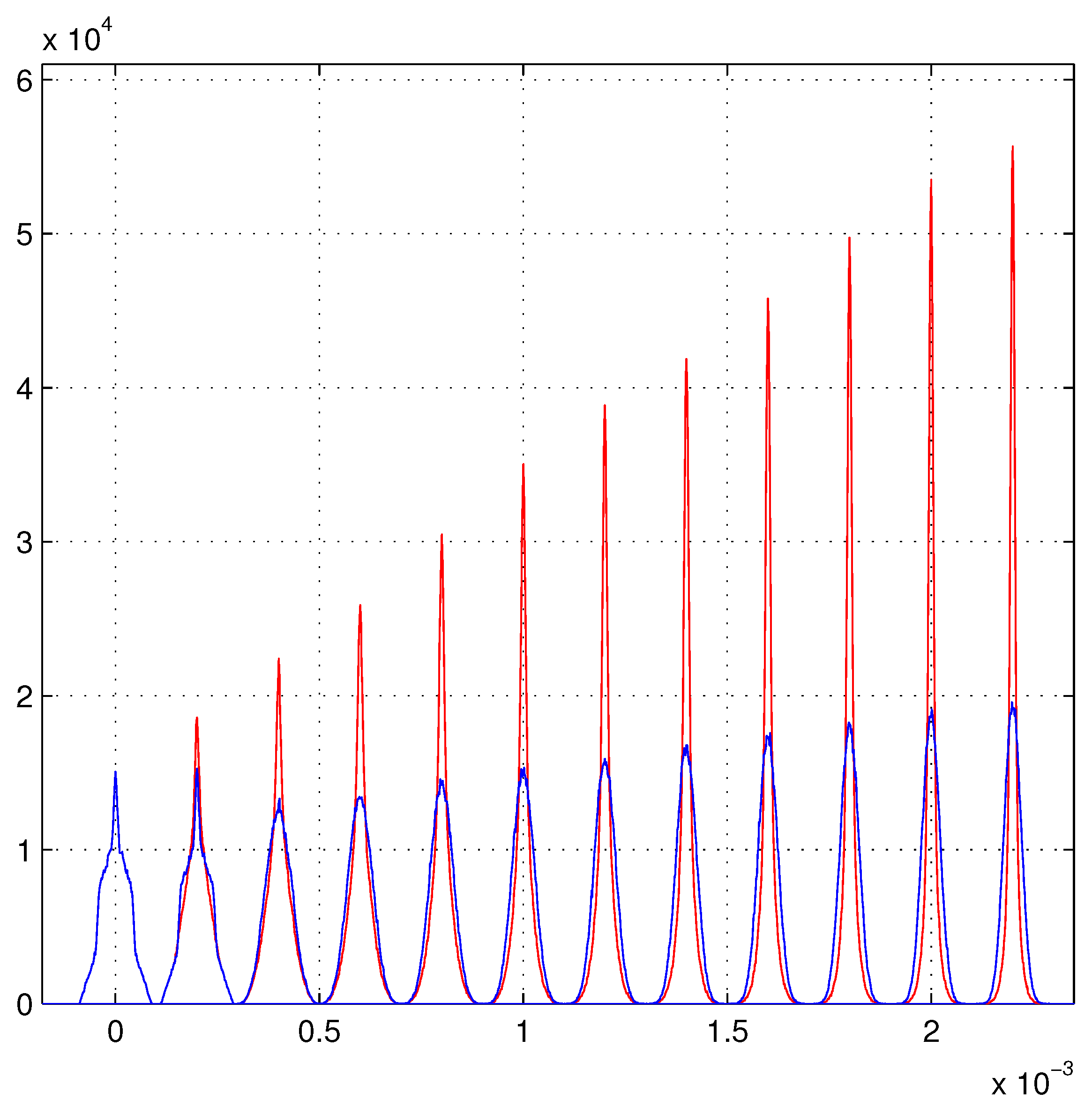
Figure 1 shows a set of fitted straight tracks in a very simple heteroscedastic model with N equidistant observations. The reported estimator is the track direction (the tangent of a small angle). The observation (measure) uncertainties are obtained with two different standard deviations that multiply a rectangular PDF ([rand-1/2] 12 in MATLAB notation) of zero mean and unit variance (minimal heteroscedasticity). One type of observation has a very small standard deviation with a lower probability 20 % , and the other of higher standard deviation and and higher probability of 80 % . The standard deviation of the observations are σ 1 = 0.18 and σ 2 = 0.018 the track length is 7063.5. The two types of observations are distributed on the straight track with a binomial PDF, this simple PDF is able to produce a large number of tracks with different sets of observations. Few lines of MATLAB [9] code suffice for this numerical proof. This model is inspired by a simplified version of a set of straight tracks in a silicon tracker.More complete simulations are in [6,8].
In the least-squares equations, the estimated parameters are multiplied by known factors defining the fitting problem, our selected factors are the positions of the detector planes or their squares (or one). This selection gives a direct physical meaning to the estimated parameters and the inequalities are among their variances. With other selections of those factors (for example orthogonal polynomials), the demonstration of the inequalities is formally identical, but the direct physical meaning of the fitted parameters is lost. The inequalities for any number of estimators can be easily obtained with simple extensions.
Section 2 defines the properties of the PDFs to be used in the developments and proves the inequalities for the straight track estimators. Section 3 is dedicated to the estimators of curved tracks. Inequalities for a generic linear set of estimators are discussed in Section 4. The effects of the inequalities on the resolutions of the reconstructed parameters are reported in Section 5. The results are summarized in Section 6. A preliminary version of this work was reported in [arXiv:2003.10021].

2. Inequalities for Irregular (and Regular) Models

The developments of [4] require very special properties for the PDFs: continuity, at least two times differentiability, inversion of derivation and integration, and others. All these properties are globally indicated as regular models. The CRF-demonstrations always introduce divisions by the PDF to define logarithmic derivatives. For finite-range PDFs, it would be very complicated to avoid divisions by zero. The set of Gaussian PDFs is a perfect example of a regular model. Instead, the rectangular PDFs (for example) lack few of the essential features of the regular models and the CRF-methods cannot be used in this case. Even the schematic (realistic) models of [6,7,8] are irregular models due to the construction of the weights as described in [7]. Hence, a different method is required to prove the variance inequalities for systems excluded by the CRF-assumptions. The fundamental differences of this approach, with respect to [4], are centered around a few crucial assumptions and developments. Other parts and the essential notations are similar to [4]. We will never write the full expressions of the used variances, these are very long equations. Extensive use of matrices allows easy manipulations of those expressions.
Pure homoscedastic systems will be neglected in the following. The systems of our interest involve elementary particles and their complex interactions with detectors. A large set of probabilistic events are allowed in these interactions. Each hit (observation) turns out to be different from any other and extended heteroscedastic models are required. Therefore, we dedicate our exclusive attention to heteroscedastic systems.

2.1. Definitions of the Probability Properties

The observations (measures) are independent random variables with f j ( x ) as PDFs. Very general mathematical properties will be supposed for the f j ( x ) , containing regular and irregular models. To simplify the notations of the integrals, the functions f j ( x ) are defined on all the real axis, even for the f j ( x ) different from zero on a finite interval. These demonstrations do not require divisions by PDFs and the addition of large sectors of zero values are harmless. In this way, the limits of the integrals can be extended from to + , and they are implied in each integral.
The properties of the f j ( x ) are (for any real θ ):
θ R : f j ( x θ ) 0 , f j ( x θ ) d x = 1 , f j ( x θ ) ( x θ ) d x = 0 , f j ( x θ ) ( x θ ) 2 d x = σ j 2 .
The case of a single estimator is irrelevant for track reconstruction and will be neglected. Its variance inequality can be easily proved with the simple use of the Cauchy–Schwarz inequality. We will directly concentrate on straight tracks. They cross N detection planes (for example micro-strips) producing the observations { x 1 , x 2 , , x N } obtained by the PDFs f j ( x j β y j γ ) . Here, β is the track impact point, and γ y j is the angular shift in a plane distant y j from the reference plane. The reference plane is selected to have j y j = 0 . The likelihood function for the N observations (hits) of the track is:
L 1 , 2 , , N ( x , β , γ ) = f 1 ( x 1 β y 1 γ ) f 2 ( x 2 β y 2 γ ) f N ( x N β y N γ ) .
Two different mean-squares of observations are defined; the standard one M s (homoscedastic) and the weighted one M w (heteroscedastic):
M s = j = 1 N ( x j β y j γ ) 2 , M w = j = 1 N ( x j β y j γ ) 2 σ j 2 .
The definition of the unbiased estimators is done through the derivatives in β and γ of M s and M w . The two required vectors are S 1 , 2 , , N ( x , β , γ ) and U 1 , 2 , , N ( x , β , γ ) :
S 1 , 2 , , N ( x , β , γ ) = 1 2 M s β M s γ = j = 1 N ( x j β y j γ ) j = 1 N ( x j β y j γ ) y j .
The condition j y j = 0 is neglected in S 1 , 2 , , N ( x , β , γ ) to maintain a similarity with U 1 , 2 , , N ( x , β , γ ) :
U 1 , 2 , , N ( x , β , γ ) = 1 2 M w β M w γ = j = 1 N ( x j β y j γ ) σ j 2 j = 1 N ( x j β y j γ ) y j σ j 2 .
The mean values of S 1 , 2 , , N ( x , β , γ ) and of U 1 , 2 , , N ( x , β , γ ) with the likelihood L 1 , 2 , , N ( x , β , γ ) are always zero for Equation (1), and identically for any of their linear combinations. The linear combinations to extract the unbiased estimators from the vector S 1 , 2 , , N ( x , β , γ ) and U 1 , 2 , , N ( x , β , γ ) are given by the following two 2 × 2 matrices R and I (from now on, the indications 1 , 2 , , N of the type of PDFs f j ( x ) will be implied):
R = 1 2 d x L ( x , β , γ ) 2 M s β 2 2 M s β γ 2 M s γ β 2 M s γ 2 = N 0 0 j = 1 N y j 2 ,
I = 1 2 d x L ( x , β , γ ) 2 M w β 2 2 M w β γ 2 M w γ β 2 M w γ 2 = j = 1 N 1 σ j 2 j = 1 N y j σ j 2 j = 1 N y j σ j 2 j = 1 N y j 2 σ j 2 .
The matrices R and I are formally identical to the Fisher information for Gaussian PDFs, homoscedastic for R and heteroscedastic for I . The integral forms of Equations (6) and (7) serve to save an analogy with [4], but they are irrelevant here. The transposed matrices are indicated as R or I . For their symmetry, we often neglect to distinguish them from their transposed.
The Gaussian model of [4] shows that the matrix elements of Equation (7) are equal to the integrals of the likelihood L ( x , β , γ ) with products of the two first derivatives of M w . This is a fundamental identity of the CRF-method [2,3], its proof requires the computation of derivatives with integrations (and division by the likelihood). Unfortunately, these commutations (and divisions) are impossible for irregular models. Instead, a direct calculation with the Equation (1) will give the last matrix of Equation (7). Before studying the variances, the unbiased estimators T 1 ( x ) , T 2 ( x ) must be defined. They are extracted from the vector U:
U ( x , β , γ ) = j = 1 N ( x j ) σ j 2 j = 1 N ( x j y j ) σ j 2 I β γ , I 1 U ( x , β , γ ) = T 1 ( x ) T 2 ( x ) β γ .
The matrix I 1 and the two estimators T 1 ( x ) , T 2 ( x ) are:
I 1 = 1 Det { I } j = 1 N y j 2 σ j 2 j = 1 N y j σ j 2 j = 1 N y j σ j 2 j = 1 N 1 σ j 2 , T 1 ( x ) T 2 ( x ) = I 1 j = 1 N ( x j ) σ j 2 j = 1 N ( x j y j ) σ j 2 .
For their special linear combinations of U components, the integrals of T 1 ( x ) and T 2 ( x ) with the likelihood L ( x , β , γ ) give β and γ :
T 1 ( x ) β L ( x , β , γ ) d x = 0 , T 1 ( x ) L ( x , β , γ ) d x = β , T 2 ( x ) γ L ( x , β , γ ) d x = 0 , T 2 ( x ) L ( x , β , γ ) d x = γ .
As previously anticipated, the direct calculation of the integrals of the mean values of the products U i U j (with Equation (1)) gives:
d x L ( x , β , γ ) · U ( x , β , γ ) U ( x , β , γ ) = j = 1 N 1 σ j 2 j = 1 N y j σ j 2 j = 1 N y j σ j 2 j = 1 N y j 2 σ j 2 ,
the matrix of Equation (11) coincides with I . This calculation does not require a double differentiation of the logarithm of the likelihood as in [4]. The variance-covariance matrix for T 1 ( x ) , T 2 ( x ) becomes:
I 1 U ( x , β , γ ) · U ( x , β , γ ) I 1 L ( x , β , γ ) d x = I 1 .
A similar procedure must be done on the vector S ( x , β , γ ) . The corresponding unbiased estimators are:
S ( x , β , γ ) = j = 1 N ( x j ) j = 1 N ( x j y j ) R β γ , R 1 S ( x , β , γ ) = T a ( x ) T b ( x ) β γ .
As previously done for other expressions, even the cross-correlation matrix of the estimators T 1 ( x ) , T 2 ( x ) and T a ( x ) , T b ( x ) is given by a direct integration of the terms in square brackets:
R 1 S ( x , β , γ ) · U ( x , β , γ ) L ( x , β , γ ) d x I 1 = R 1 N 0 0 j = 1 N y j 2 I 1 = I 1 .
These results are identical to those obtained in [4] for Gaussian PDFs with a commutation of integrations and derivatives (allowed only for regular models). In this approach, they are derived with the sole use of the Equation (1), therefore, valid for irregular and regular models.

2.2. The Variance Inequalities

In the following, we abandon the complex use of positive semi-definite matrices of [3,4]. The Cauchy–Schwarz inequality will be directly applied. The matrix of Equation (14) contains the integral:
T a ( x ) β T 1 ( X ) β L ( x , β , γ ) d x = ( I 1 ) 1 , 1 ,
which implies the following Cauchy–Schwarz inequality (with the trivial substitution of the likelihood L = L L ):
T a ( x ) β 2 L ( x , β , γ ) d x T 1 ( X ) β 2 L ( x , β , γ ) d x > ( I 1 ) 1 , 1 2 .
The equality is excluded because T a ( x ) and T 1 ( x ) are never proportional for N > 2 (and true heteroscedastic systems). For N = 2 , the minimums of M w and M s coincide (as their variances). We use this condition in Figure 1 to check the consistency of the code. Equation (12) states that the matrix element ( I 1 ) 1 , 1 is just the variance of T 1 ( x ) , therefore, the inequality becomes:
T a ( x ) β 2 L ( x , β , γ ) d x ( I 1 ) 1 , 1 > ( I 1 ) 1 , 1 2 = j ( y j 2 / σ j 2 ) j ( y j 2 / σ j 2 ) k ( 1 / σ k 2 ) ( j y j / σ j 2 ) 2 2 , j σ j 2 N 2 = T a ( x ) β 2 L ( x , β , γ ) d x > T 1 ( x ) β 2 L ( x , β , γ ) d x .
The inequality for T b ( x ) and T 2 ( x ) is obtained as in Equations (15)–(17) with the matrix element ( I 1 ) 2 , 2 :
T b ( x ) γ 2 L ( x , β , γ ) d x ( I 1 ) 2 , 2 > ( I 1 ) 2 , 2 2 = j ( 1 / σ j 2 ) j ( y j 2 / σ j 2 ) k ( 1 / σ k 2 ) ( j y j / σ j 2 ) 2 2 , j y j 2 σ j 2 ( k y k 2 ) 2 = T b ( x ) γ 2 L ( x , β , γ ) d x > T 2 ( x ) γ 2 L ( x , β , γ ) d x .
Again, the equality is excluded because T a ( x ) and T 1 ( x ) are never proportional for N > 2 .
Up to this point, we supposed the absence of any effective variance in the standard least-squares method. Often, the difference of detector technologies is introduced with a global effective variance σ a l for each hit in a detector layer (as in [10]). It is easy to demonstrate that the precedent inequalities continue to be valid even in this case. In fact, the correct likelihood attributes to each hit its optimized variance, and this overrides the global effective variance. This demonstration introduces small modifications with respect to the previous one, essentially, the R matrix contains now all these modifications. In any case, the cross-correlation matrix is always generated by the product R 1 R I 1 . An extended demonstration also containing this case is reported in Section 4.

3. Extension of Inequalities to Momentum Estimators

More important than the estimators for the straight tracks, are the estimators for fits of curved tracks in the magnetic field. Therefore, we will calculate these inequalities for general irregular (and regular) models. We will limit to a simpler case of high-momentum charged particles in a tracker with a homogeneous magnetic field, orthogonal to the particle track. Beyond a given momentum (depending from the detector and the magnetic field) a segment of parabola approximates a segment of a circular path with negligible relative error [7]. If the parabolic approximation would be insufficient, a method of successive linearizations (as in [11]) can be used, or the unknowns can be extracted from Equation (19) (with the due extensions) as done in [7]. As for straight tracks, the standard least-squares fit and the weighted one will be compared. The likelihood function with the addition of curvature η for the N observations is:
L ( x , β , γ , η ) = f 1 ( x 1 β y 1 γ y j 2 η ) f 2 ( x 2 β y 2 γ y j 2 η ) f N ( x N β y N γ y N 2 η ) .
The two mean squares of observations, M s (homoscedastic) and M w (heteroscedastic), are:
M s = j = 1 N ( x j β y j γ y j 2 η ) 2 M w = j = 1 N ( x j β y j γ y j 2 η ) 2 σ j 2 .
The definition of the unbiased estimators requires the introduction of the vectors S ( x , β , γ , η ) and U ( x , β , γ , η ) :
S ( x , β , γ . η ) = 1 2 M s β M s γ M s η = j = 1 N ( x j β y j γ y j 2 η ) j = 1 N ( x j β y j γ y j 2 η ) y j j = 1 N ( x j β y j γ y j 2 η ) y j 2 .
To save the similarity with the form of U ( x , β , γ , η ) , the condition j y j = 0 is not implemented. The vector U ( x , β , γ , η ) is:
U ( x , β , γ , η ) = 1 2 M w β M w γ M w η = j = 1 N ( x j β y j γ y j 2 η ) σ j 2 j = 1 N ( x j β y j γ y j 2 η ) y j σ j 2 j = 1 N ( x j β y j γ y j 2 η ) y j 2 σ j 2 .
To extract the unbiased estimators, the following two matrices are required:
R = 1 2 d x L ( x , β , γ . η ) 2 M s β 2 2 M s β γ 2 M s β η 2 M s γ β 2 M s γ 2 2 M s γ η 2 M s η β 2 M s η γ 2 M s η 2 = N 0 j y j 2 0 j y j 2 j y j 3 j y j 2 j y j 3 j y j 4 ,
I = 1 2 d x L ( x , β , γ , η ) 2 M w β 2 2 M w β γ 2 M w β η 2 M w γ β 2 M w γ 2 2 M w γ η 2 M w η β 2 M w η γ 2 M w η 2 = j 1 / σ j 2 j y j / σ j 2 j y j 2 / σ j 2 j y j / σ j 2 j y j 2 / σ j 2 j y j 3 / σ j 2 j y j 2 / σ j 2 j y j 3 / σ j 2 j y j 4 / σ j 2 .
As above, the integrations with the likelihood are irrelevant. On these irregular (and regular) models, the integrations of products of S · S and U · U must be performed on their Forms (21) and (22).
The vectors U and S give the unbiased estimators T 1 , T 2 , T 3 and T a , T b , T c :
U ( x , β , γ , η ) = j = 1 N ( x j ) σ j 2 j = 1 N ( x j y j ) σ j 2 j = 1 N ( x j y j 2 ) σ j 2 I β γ η , I 1 U ( x , β , γ η ) = T 1 ( x ) T 2 ( x ) T 3 ( x ) β γ η ,
S ( x , β , γ , η ) = j = 1 N ( x j ) j = 1 N ( x j y j ) j = 1 N ( x j y j 2 ) R β γ η , R 1 S ( x , β , γ ) = T a ( x ) T b ( x ) T c ( x ) β γ η .
The direct integrations of the products U i · U j with the likelihood give:
d x L ( x , β , γ , η ) · U ( x , β , γ , η ) U ( x , β , γ , η ) = I ,
and the variance–covariance matrix of T 1 , T 2 and T 3 becomes:
I 1 d x L ( x , β , γ , η ) U ( x , β , γ , η ) · U ( x , β , γ , η ) I 1 = I 1 .
The cross-correlation matrix of the estimators T 1 ( x ) , T 2 ( x ) , T 3 ( x ) and T a ( x ) , T b ( x ) , T c ( x ) is given by a direct calculations of the integrals. The integrations in the square brackets give R :
R 1 S ( x , β , γ , η ) · U ( x , β , γ , η ) L ( x , β , γ , η ) d x I 1 = R 1 R I 1 = I 1
and the cross-correlation of T c ( x ) with T 3 ( x ) , the unbiased estimators of the curvature, is:
T c ( x ) η T 3 ( X ) η L ( x , β , γ , η ) d x = ( I 1 ) 3 , 3 .
Equation (30) produces a Cauchy–Schwarz inequality: (remembering that the likelihood can be written as L = L L ):
T c ( x ) η 2 L ( x , β , γ , η ) d x T 3 ( X ) η 2 L ( x , β , γ , η ) d x > ( I 1 ) 3 , 3 2 ,
the equality is excluded because T c ( x ) and T 3 ( x ) are never proportional for N > 3 . For N = 3 , the minima of M w and M s coincide. For Equation (29), the matrix element ( I 1 ) 3 , 3 is the variance of T 3 ( x ) . Therefore, the inequality for the curvature becomes:
T c ( x ) η 2 L ( x , β , γ , η ) d x ( I 1 ) 3 , 3 > ( I 1 ) 3 , 3 2 , T c ( x ) η 2 L ( x , β , γ , η ) d x > T 3 ( x ) η 2 L ( x , β , γ , η ) d x .
This inequality extends the validity of the results of our simulations of [7] to any heteroscedastic system. The inequalities for β and γ can be obtained with a similar procedure.
These demonstrations are directly extendible to a number of parameters greater than those considered here. The fundamental element for these inequalities is the identity of the variance–covariance matrix for the estimators { T 1 ( x ) , T 2 ( x ) , T 3 ( x ) } and the cross-covariance with the other estimators.

4. Generalized Inequalities for any Linear Estimators

The previous developments concentrated the attention to inequalities involving forms of the standard least-squares method. The simplicity of the expressions for the parameter estimators in the standard least-squares could raise the doubt that more complex linear forms of the estimators (as those produced by the Kalman filter) are able to have lower variances than the proper heteroscedastic least-squares. We will prove that any other set of linear estimators has higher variances. For simplicity, this proof will be limited to two estimators, but it can be easily extended. The properties of the PDFs of the observations are those of Equation (1) and the heteroscedastic likelihood function is that of Equation (2):
L ( x , β , γ ) = f 1 ( x 1 β y 1 γ ) f 2 ( x 2 β y 2 γ ) f N ( x N β y N γ ) .
The first mean squares of the observations of Equation (3) is modified in a M g 1 to give a general linear combination of estimators. This linear combination implies N free parameters. With another mean square of observation M g 2 , it is easy to produce a linear combination with 2N free parameters, saving the unbiasedness of the estimators:
a j > 0 , M g 1 = j = 1 N a j ( x j β y j γ ) 2 ; b j > 0 , M g 2 = j = 1 N b j ( x j β y j γ ) 2 .
To eliminate trivial results we pose N > 2 and a j , b j 1 / σ j 2 and b k a k for at least one j and a k. The unbiased estimators are extracted from the derivatives of M g 1 , M g 2 and M w defining the two vectors G ( x , β , γ ) and U ( x , β , γ ) :
G ( x , β , γ ) = 1 2 M g 1 β M g 2 γ = j = 1 N a j ( x j β y j γ ) j = 1 N b j ( x j β y j γ ) y j .
The vector U ( x , β , γ ) is (Equation (5)):
U ( x , β , γ ) = 1 2 M w β M w γ = j = 1 N ( x j β y j γ ) σ j 2 j = 1 N ( x j β y j γ ) y j σ j 2 .
As for the vector U ( x , β , γ ) , the mean values of G ( x , β , γ ) with the likelihood L ( x , β , γ ) is always zero for Equation (1), and identically for any of their linear combinations. The linear combinations to extract the unbiased estimators from the vector G ( x , β , γ ) are given by the following 2 × 2 matrix K :
K = 1 2 d x L ( x , β , γ ) 2 M g 1 β 2 2 M g 1 β γ 2 M g 2 γ β 2 M g 2 γ 2 = j a j j a j y j j b j y j j b j y j 2 ,
and I of Equation (7):
I = 1 2 d x L ( x , β , γ ) 2 M w β 2 2 M w β γ 2 M w γ β 2 M w γ 2 = j 1 σ j 2 j y j σ j 2 j y j σ j 2 j y j 2 σ j 2 .
The definition of the unbiased estimators for the U vector is in Equations (8)–(10). The variance–covariance matrix for the unbiased estimators of U is calculated in Equations (11) and (12) giving I 1 . The unbiased estimators from the vector G are:
G ( x , β , γ ) = j ( a j x j ) j ( b j x j y j ) K β γ , K 1 G ( x , β , γ ) = T d ( x ) T e ( x ) β γ .
The cross-correlation matrix of the estimators T 1 ( x ) , T 2 ( x ) and T d ( x ) , T e ( x ) is given by a direct integrations of the terms in square brackets:
K 1 [ G ( x , β , γ ) · U ( x , β , γ ) L ( x , β , γ ) d x ] I 1 = K 1 j a j j a j y j j b j y j j b j y j 2 I 1 = I 1 .
The cross-correlation is the symmetric matrix I 1 and it is identical to the variance–covariance matrix of the estimators T 1 ( x ) and T 2 ( x ) . This identity, obtained before for different estimators, is the key point of the demonstration. Given this identity, the inequality is immediate; the matrix of Equation (40) contains the integral:
T d ( x ) β T 1 ( X ) β L ( x , β , γ ) d x = ( I 1 ) 1 , 1 ,
which implies the following Cauchy–Schwarz inequality (with the trivial substitution of the likelihood L = L L ):
T d ( x ) β 2 L ( x , β , γ ) d x T 1 ( X ) β 2 L ( x , β , γ ) d x > ( I 1 ) 1 , 1 2 .
Due to the identity of the variance–covariance of estimators T 1 ( x ) and T 2 ( x ) and the cross-covariance with the estimators T d ( x ) and T e ( x ) , the inequality is obtained:
T d ( x ) β 2 L ( x , β , γ ) d x ( I 1 ) 1 , 1 > ( I 1 ) 1 , 1 2 , T d ( x ) β 2 L ( x , β , γ ) d x > T 1 ( x ) β 2 L ( x , β , γ ) d x .
The variance of the estimator T d ( x ) is always greater than the variance of T 1 ( x ) . The inequality for T e ( x ) and T 2 ( x ) is obtained with precedent equations and the matrix element ( I 1 ) 2 , 2 :
T e ( x ) γ 2 L ( x , β , γ ) d x ( I 1 ) 2 , 2 > ( I 1 ) 2 , 2 2 , T e ( x ) γ 2 L ( x , β , γ ) d x > T 2 ( x ) γ 2 L ( x , β , γ ) d x .
The variance of the estimator T e ( X ) is always greater than the variance of T 2 ( X ) . Therefore, these very unusual estimators with their 2N free parameters are always non-optimal compared to the heteroscedastic least-squares.
The extension to three or more estimators can be done in an analogous way. In any case, the properties of the likelihood dominate the demonstrations producing always the identity among the matrix of the variance-covariance and the cross-covariance.

5. Effects of the Inequalities on the Resolution of the Estimators

Up to this point, we discussed the formal proofs of variance inequalities, and illustrated their effects in Figure 1. In the following, we will show the direct connections of the variance inequalities to the line-shapes of Figure 1 and to the corresponding figures of [4,8]. To simplify the notations, we will take β and γ equal to zero (as in the simulations). It must be recalled that the illustrated simulations deal with a large number of tracks with different successions of hit quality ( σ j 1 , , σ j N ). For each succession of σ j 1 , , σ j N , extracted from the allowed set of { σ k } , we have a definite form of the estimators T 1 ( x ) and T 2 ( x ) (weighted least-squares). Instead, T a ( x ) and T b ( x ) (standard least-squares) are formally invariant. The studied estimator is the track direction γ , thus T 2 ( x ) and T b ( x ) are the selected estimators. These demonstrations can be easily extended to other estimators.

5.1. The Line-Shapes of the Estimators T 2 ( x ) and T b ( x )

For any set of observations x j 1 , , x j N , the estimator T 2 ( x ) gives a definite value γ * . The set of all possible γ * has the probability distribution P j 1 , , j N ( γ * ) (with the method of [5,7]):
P j 1 , , j N ( γ * ) = d x δ γ * T 2 ( σ j 1 , σ j N , x ) f j 1 ( x 1 ) f j 2 ( x 2 ) f j N ( x N ) .
Due to the linearity of T 2 in the observations x , this integral gives a weighted convolution of the functions f j 1 ( x 1 ) f j 2 ( x 2 ) f j N ( x N ) . For the convolution theorems [12], the variance of P j 1 , , j N ( γ * ) is given by the ( I 1 ) 2 , 2 of Equation (12) with the corresponding σ j :
Σ j 1 , , j N = ( I 1 ) 2 , 2 .
In the case of [4,8], the convolution of Gaussian PDFs gives another Gaussian function with the variance Σ j 1 , , j N , therefore P j 1 , , j N ( γ * ) becomes:
P j 1 , , j N ( γ * ) = exp [ γ * 2 2 Σ j 1 , , j N ] 1 2 π Σ j 1 , , j N .
The mean value of P j 1 , , j N ( γ * ) is zero, as it must be for the unbiasedness of the estimator, and its maximum is 1 / 2 π Σ j 1 , , j N .
A similar procedure of Equations (45)–(47) can be extended to the standard least-squares with the due differences T 2 T b , ( I 1 ) 2 , 2 ( R 1 ) 2 , 2 and P j 1 , , j N ( γ * ) P j 1 , , j N b ( γ b * ) ( R 1 is the variance-covariance matrix of the standard fit). In this case the variance of the convolution is defined:
S j 1 , , j N = ( R 1 ) 2 , 2
and, for Gaussian PDFs, the probability P j 1 , , j N b ( γ b * ) is the function:
P j 1 , , j N b ( γ b * ) = exp [ γ b * 2 2 S j 1 , , j N ] 1 2 π S j 1 , , j N .
The maximum of P j 1 , , j N b ( γ b * ) is 1 / 2 π S j 1 , , j N . For the inequality (18), it is:
1 / 2 π S j 1 , , j N 1 / 2 π Σ j 1 , , j N .
The equality is true if, and only if, all the σ j of the track are identical. Now this condition must be inserted for the randomization of the { σ j } . In the weighted fits, the law of large numbers determines the convergence of the line-shape toward the function:
Π ( γ * ) = j 1 , , j N p j 1 , , j N P j 1 , , j N ( γ * ) , j 1 , , j N p j 1 , , j N = 1 .
Analogously for the standard fits:
B ( γ b * ) = j 1 , , j N p j 1 , , j N P j 1 , , j N b ( γ b * ) .
The probability of the sequence of hit quality is p j 1 , , j N . The law of large numbers gives even an easier way for an analytical calculation of the maximums of the two distributions:
Π ( 0 ) = lim M 1 M k = 1 M 1 / 2 π Σ k B ( 0 ) = lim M 1 M k = 1 M 1 / 2 π S k ,
where the index k indicates a track of a large number of simulated tracks, Σ k is the corresponding variance calculated as in the definition of ( I 1 ) 2 , 2 and S k with the expression ( R 1 ) 2 , 2 . The inequality (50) assures that Π ( 0 ) > B ( 0 ) . For our 150,000 tracks the convergence of the maximums of the empirical PDFs to Equation (53) is excellent for Gaussian PDFs. For the rectangular PDFs of Figure 1, the results of Equation (53) are good for the standard fit but slightly higher for weighted fits (3∼4%). The strong similarity of the line-shapes of the rectangular PDFs with the Gaussian PDFs is due to the convolutions among various functions f j ( x ) that rapidly tend to approximate Gaussian functions (Central Limit Theorem). The weighted convolutions of Equation (45) has higher weights for the PDFs of good hits. These contribute mostly to the maximum of the line-shape. Unfortunately, the good hits have a lower probability and the lower number of the convolved PDFs produce the worst approximation to a Gaussian than in the case of standard fit. In fact, in the probability P j 1 , , j N b ( γ b * ) of the standard fit, the weights of the convolved functions are identical and the convergence to a Gaussian is better (for N not too small). Better line-shapes, for non-Gaussian PDFs, can be obtained with the approximations of [13] for doing convolutions.

5.2. Resolution of Estimators

Figure 1 evidences the large differences of the γ * -PDFs of the weighted least-squares fits compared to the γ b * -PDFs of the standard fits. For N > 3 the PDFs of the standard fits are very similar to Gaussian. Instead, the PDFs of the weighted fits are surely non-Gaussian. The definition of resolution becomes very complicated in these cases. In our previous papers, we always used the maximums of the PDFs to compare the resolution of different algorithms. Our convention may be criticized on the ground of the usual definition as the standard deviation of all the data. The weakness of this position is evident for non-Gaussian distributions. In fact, the standard deviation (as the variance), for non-Gaussian PDF, is mainly controlled by the tails of the distributions. Instead, the maximums are not directly affected by the tails and they are true points of the PDFs. We have to recall that the preference of the standard deviation is inherited from the low-statistics of the pre-computer era (when the maximums of data distributions were impossible to obtain). The long demonstrations about the Bessel correction ( 1 / ( n + 1 ) in place of 1 / n ) were relevant for the low-statistics, but absolutely irrelevant for our large numbers of data. In addition to this, a decreasing resolution, when the resolving power of the algorithm/detector increases, easily creates contradictory statements.
Let us justify our preference. The resolution indicates a property of an algorithm/instrument to discriminate near values of the calculated/measured parameters (for example two near tracks). Clearly, the maximum resolving power is obtained if the response of the algorithm/instrument is a Dirac δ -function. In this case, the parameters (the two near tracks) are not resolved if, and only if, they coincide. Therefore, the algorithm with the best resolution is the one with the better approximation of a Dirac δ -function. Among a set of responses, it is evident that the response with the highest maximum is the better approximation of a Dirac δ -function and thus that with the largest resolution. This is the reason for our selection. However, our preference is a “conservative” position. In fact, in recent years it is easy to find, in literature, other “extremist” conventions. A frequent practice (as in [14] or in Figure 18 of [15]) is to fit the central part (the core) of the distribution with a piece of Gaussian and to take the standard deviation of this Gaussian as the measure of the resolution.
The Gaussian toy model allows us to calculate the variance of a Gaussian fitted to the core of the PDFs. A method to fit a Gaussian is to fit a parabola to the logarithm of the set of data. The second derivative of the parabola, at the maximum of the distribution, is the inverse of the variance of the Gaussian. This variance can be obtained by the function Π ( γ * ) of Equations (51) and (53):
1 Σ e f f = d 2 ln Π ( γ * ) d γ * 2 | γ * = 0 = lim M k = 1 M 1 / Σ k 3 n = 1 M 1 / Σ n .
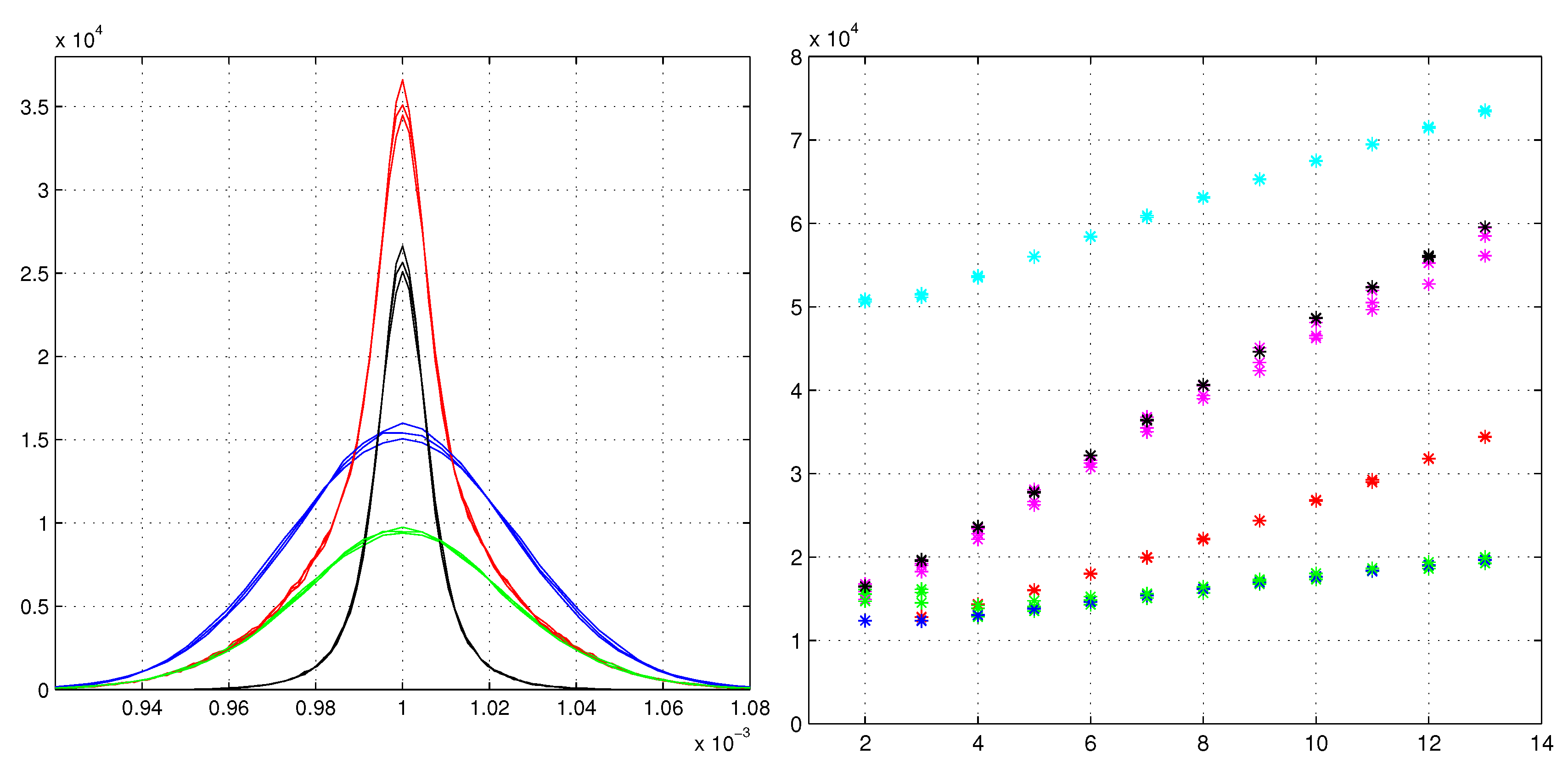
The common factors are eliminated in the last fraction. Gaussian functions, with standard deviations Σ e f f , reproduce well the core of Π ( γ * ) even if the Gaussian rapidly deviates from Π ( γ * ) . Instead, the Gaussian functions, with the height coinciding with Π ( 0 ) , are outside the core of Π ( γ * ) , their full width at half maximum is always larger. Figure 2 illustrates a few of these aspects for three different toy models.
The left side of Figure 2 reports the line-shapes for N = 7 layers of the three toy models: the Gaussian of [4,8], the rectangular of Figure 1 and a toy model with triangular PDFs. These three types of PDFs are those considered by Gauss in his paper of 1823 [11] on the least-squares method. The line-shapes are almost identical with small differences in their maximums. The red line-shapes are formed by the sums of the black and the green lines, respectively the fraction of the red ones given by the tracks with two or more good hits, and the fraction given by tracks with less than two good hits. The heights of the red lines have essential contributions from the black distributions. The line-shapes with the lowest maximums are those of the rectangular toy model and the highest maximums are those of the Gaussian toy model.
The right side of Figure 2 compares the various parameters as effective heights 1 / 2 π Σ l (like Gaussian PDFs with variance Σ l ) and the maximums of the real empirical PDFs. For the standard fits, only the Σ l corresponding to the variances are reported (blue asterisks). The green asterisks are the maximums of the blue lines of Figure 1. Excluding the cases N = 2 and N = 3, the two heights are almost coincident. The case N = 2 is dealt with in Section 2.2. For N = 3, the standard fit tends to have very similar estimators to those of N = 2, this is due to y 2 = 0 that suppresses the central observations. Instead for the heteroscedastic fit, the reported heights 1 / 2 π Σ l are largely different. The red asterisks have Σ l as the variance of the three simulated distributions, the magenta asterisks are the maximums of the three histograms. The black asterisks are the Π ( 0 ) of Equation (53). The highest (cyan) asterisks are the Σ l from Equation (54). Equation (54) has the form of weighted mean of the inverse of the variance of P j 1 , , j N ( γ * ) , with a weight proportional to the maximum of its P j 1 , , j N ( γ * ) . This form allows its extension to rectangular and triangular toy models even if their derivatives could be problematic. However, these fitted Gaussian PDFs are slightly too narrow for the non-Gaussian toy models, so we applied a small reduction (0.87) to the cyan heights to have a better fit with the rectangular toy models with N ≥ 7. We calculated 1 / 2 π Σ e f f of Equation (54) even for the standard fit (not reported in Figure 2). The cases with N = 2 and N = 3 are identical to the case of the Gaussian toy model, but these heights drop rapidly converging to the green asterisks of Figure 2 for N ≥ 6. Hence, coming back to the resolution, the gain in resolution, with respects to the homoscedastic fit, has values: 1.34, 2.4 and 4.1, for the model with seven detecting layers. Waiting for a general convention to define the resolution in these non-Gaussian distributions, our preferred value is 2.4 times the result of the standard fit. However, it is better to correlate the obtained line-shapes to physical parameters of the problem. In [7], we used the magnetic field and the signal-to-noise ratio to measure the fitting improvements.
Lastly, we have to remember that the non-Gaussian models allow a further increase in resolution with the maximum-likelihood search. Authors in [6,7] show the amplitude of the increase in resolution due to the maximum-likelihood search. If the triangular and rectangular toy models had similar improvements, the Gaussian-model would be the worst of all.
6. Conclusions

Inequalities among variances of the least-squares estimators are calculated for heteroscedastic systems. They demonstrate that the weighted least-squares method has minimal variance. Thus, it is optimal according to the usual definition of optimality. Instead, the standard least-squares method, of large use, is not the optimal selection for heteroscedastic fits. These developments are explicitly constructed for irregular models that can not be handled with the Cramer–Rao-Frechet approach. However, the conditions imposed on the probability density functions are valid even for regular models. Thus, any mixtures of regular and irregular models are equally dealt with in these studies. The linearity of the estimators are key features for the demonstrations. To test the amplitudes of the improvements due to these inequalities, the results of simulations with one irregular models are reported. The simulations have the probability density functions of rectangular forms. This form is used as an example of the probability model intractable with the Cramer–Rao–Frechet method. A general linear least-squares model is also compared with the heteroscedastic fit, and the likelihood function of the heteroscedastic system attributes a greater variance to this general model. All these inequalities support a strong necessity of accurate models for the probabilities of the observations. The effects of the proven inequalities are connected to the formation of the line-shape of the figures. The probability distributions for the direction estimators are defined in the two different fitting methods. The law of large numbers is used to reconstruct the maximums of the plotted distributions. For the Gaussian distributions, the agreement is excellent. For the rectangular distributions, slight differences are observed.

Author Contributions

The authors contributed equally to this work. All authors have read and agreed to the published version of the manuscript.

Funding

This research did not receive external funding.

Conflicts of Interest

The authors declare no conflict of interest.

Abbreviations

The following abbreviations are used in the text.
CRFCramer–Rao–Frechet
PDFProbability density function

References

  1. Tanabashi, M.; et al. Review of Particle Physics. Phys. Rev. D 2018, 98, 030001. [Google Scholar] [CrossRef] [Green Version]
  2. Ivchenko, G.; Medvedev, Y. Mathematical Statistics; Mir: Moscow, USSR, 1990. [Google Scholar]
  3. Amemiya, T. Advanced Econometrics; Harvard University Press: Cambridge, MA, USA, 1985. [Google Scholar]
  4. Landi, G.; Landi, G.E. The Cramer-Rao inequality to improve the resolution of the least-squares method in track fitting. Instruments 2020, 4, 2. [Google Scholar] [CrossRef] [Green Version]
  5. Landi, G.; Landi, G.E. Probability distributions of positioning errors for some forms of center-of-gravity algorithms. arXiv 2020, arXiv:2004.08975. [Google Scholar]
  6. Landi, G.; Landi, G.E. Improvement of track reconstruction with well tuned probability distributions. arXiv 2014, arXiv:1404.1968. [Google Scholar]
  7. Landi, G.; Landi, G.E. Optimizing momentum resolution with a new fitting method for silicon-strip detectors. Instruments 2018, 2, 22. [Google Scholar] [CrossRef] [Green Version]
  8. Landi, G.; Landi, G.E. Beyond the N -limit of the least-squares resolution and the lucky-model. arXiv 2018, arXiv:1808.06708. [Google Scholar]
  9. MATLAB 2020a; The MathWorks Inc.: Natick, MA, USA, 2020.
  10. Hartmann, F. Silicon tracking detectors in high-energy physics. Nucl. Instrum. Methods Phys. Res. Sect. A 2012, 666, 25–46. [Google Scholar] [CrossRef]
  11. Gauss, C.F. Methode de Moindre Carre. Memoires sur la Conbination des Observation; Mallet-Bachelier: Paris, France, 1855; Available online: https://books.google.it/books?id=_qzpB3QqQkQC (accessed on 25 October 2020).
  12. Champeney, D.C. A Handbook of Fourier Theorems; Cambridge University Press: Cambridge, UK, 1987. [Google Scholar]
  13. Landi, G. Properties of the center of gravity as an algorithm for position measurements. Nucl. Instrum. Methods Phys. Res. Sect. A 2002, 485, 698–719. [Google Scholar] [CrossRef] [Green Version]
  14. Sirunyan, A.M.; et al. Performance of the reconstruction and identification of high-momentum muons in proton proton collision at s = 13 TeV. J. Instrum. 2020, 15, P02027. [Google Scholar] [CrossRef]
  15. Sirunyan, A.M.; et al. The performance of the CMS muon detector in proton-proton collision at s = 7 TeV at the LHC. J. Instrum. 2013, 8, P11002. [Google Scholar] [CrossRef]
Figure 1. Track fits for rectangular positioning errors (irregular model). Empirical probability density functions (PDFs) of the track directions for a set of tracks with N = 2 to N = 13 (heteroscedastic) observations. The PDFs for N = 2 are centered on zero, the others are shifted by N-2 steps of fixed amplitude. Blue lines: PDFs of the standard least-squares. Red lines: PDFs of the weighted least-squares. The reported dimensions are pure numbers.
Physics 02 00035 g001
Figure 2. Left plot: Empirical PDF of the fitted (straight) track direction for a tracker model with N = 7 detecting layers. Red and blue lines as in Figure 1. Black line, the fraction of red PDF due to tracks with two or more good hits. Green line: the fraction of the red PDF due to one or zero good hits The right plot reports the heights 1 / 2 π Σ l where Σ l is a variance for each N = { 2 , , 13 } . The variances Σ l are: blue asterisks: variance of standard fits, red asterisks variances of weighted fits. Cyan asterisks: the variance Σ e f f (weighted fit). Magenta asterisks maximums of red line of Figure 1 (even for Gaussian and triangular toy models), green asterisks maximums of the blue lines of Figure 1, black asterisks: the results of Π ( 0 ) .
Physics 02 00035 g002
Publisher’s Note: MDPI stays neutral with regard to jurisdictional claims in published maps and institutional affiliations.