1. Introduction
Semiconductors are materials with temperature-dependent electrical conductivity, with conductivities ranging between those of conductors (e.g., Cu) and those of insulators (e.g., SiO
2) [
1,
2,
3]. This characteristic property is the result of their incomplete (doped) crystal structure, which generally causes a decrease in their resistivity (and thus an increase in their conductivity) with an increase in temperature, in contrast to the typical behavior of metals [
4]. Semiconductors have a range of useful properties, such as facilitating the transit of current in one direction rather than in the other, providing differential resistance, and exhibiting sensitivity to light or heat [
3]. Given that their electrical properties are dependent either on doping or on the effect of electrical fields or light, semiconductor devices are widely used for applications such as amplification, switching and energy conversion, and have led to the development of transistors, integrated circuits, radio receivers, and many other communication devices [
2,
3]. Research in the field of semiconductors is, by definition, characterized by high levels of complexity due to their deviation from typical crystal structures that causes their temperature-dependent conductivity [
5]. Therefore, the modern conceptualization and understanding of semiconductor properties builds on quantum physics and other fields of complexity science to explain the nonlinear charge-carrier behavior within crystal lattice structures [
3,
5]. The relationship between voltage and current in metallic conductors is linear, and the same is true for semiconductors with low current or voltage values. At higher values, though, this relationship becomes nonlinear. A special case appears when the phenomenon of negative differential resistance (NDR), in which voltage decreases as the current increases, appears in the linear region. When this change is abrupt, the switching effect takes place [
6,
7,
8].
For instance, the ternary (i.e., consisting of three different elements) semiconductor TLMX
2 [
8], with M=Ga (Gallium) and In (Indium), and X=Se (Selenium), S (Sulfur) and Te (Tellurium), as well as the TLInX
2–TLSmX
2 alloys [
9], with X=S, Se, or Te, exhibit nonlinear effects on their current-voltage (
I-
V) characteristics (including a region of negative differential resistance), switching, and memory effects [
6,
7,
8]. The electrical conductivity of several chain-type crystals exhibits time oscillations and intermittency [
6,
7,
8,
10]. These nonlinear effects, such as negative differential resistance, are the result of an electro-thermal mechanism [
6,
7,
10]. The switching occurs because of deviations in the uniform distribution of the imperfection. Chain-type structures permit the generation of high current density filaments that act as channels between the two electrodes. Because of Joule heating, two parallel resistors exist—one high and one low. The high current density leads to Joule heating, and because of Joule heating the resistor becomes smaller. This process produces an S-type
I-
V characteristic [
6,
7,
10]. Due to the instabilities in carrier diffusion and recombination, chaotic oscillations occur [
6,
7].
Within this context, nonlinear conceptualizations in research related to semiconductors have been evident in the literature for almost three decades [
1,
3,
4], with respect to aspects such as structure [
2], dynamics [
2,
11,
12], optical behavior [
11,
13], energy applications [
14], and physical properties [
2,
15]. Indicatively, the characteristic approaches in semiconductor research are built on nonlinear stochastic processes [
11], quantum physics modeling of conductivity in semiconductors [
3,
5], nonlinear and chaotic time-series analysis [
5,
6,
7,
13], and the structural modeling of super-lattice topologies [
12]. Among such approaches, there are a couple of works that use the network paradigm to deal with the issues of complexity that govern either structural or functional connectivity in semiconductors, such as the work of [
16], who introduced the application of queuing network models for the design and analysis of semiconductor wafer fabs, and the more recent work of [
17], who applied complex network analysis to study cluster synchronization in mutually coupled semiconductor laser (SLs) networks with complex topologies. Although these examples are obviously not enough to support, epistemologically, the contribution of network science [
18,
19] to the established field of semiconductor research, they appear to have the merit of highlighting the potential linkage between these two research fields that is defined by their common area, that is, dealing with complex systems and complexity in general.
Network science is a modern discipline, using the network paradigm to model communication systems into pair-sets of nodes and links, and it has been proven as a fruitful field of interdisciplinary research, providing insights into the structure and functionality of complex interconnected systems [
18,
19]. For instance, the contribution of network science to time-series analysis has led to the research field of “complex network analysis of time-series”, which enjoys several applications in various disciplines and fields of science [
20]. This research field deals with methods for transforming a time-series into complex networks, which allows for managing a time-series with a higher complexity level by studying the topological properties of graphs instead of the time-series’ structural properties [
21,
22,
23,
24,
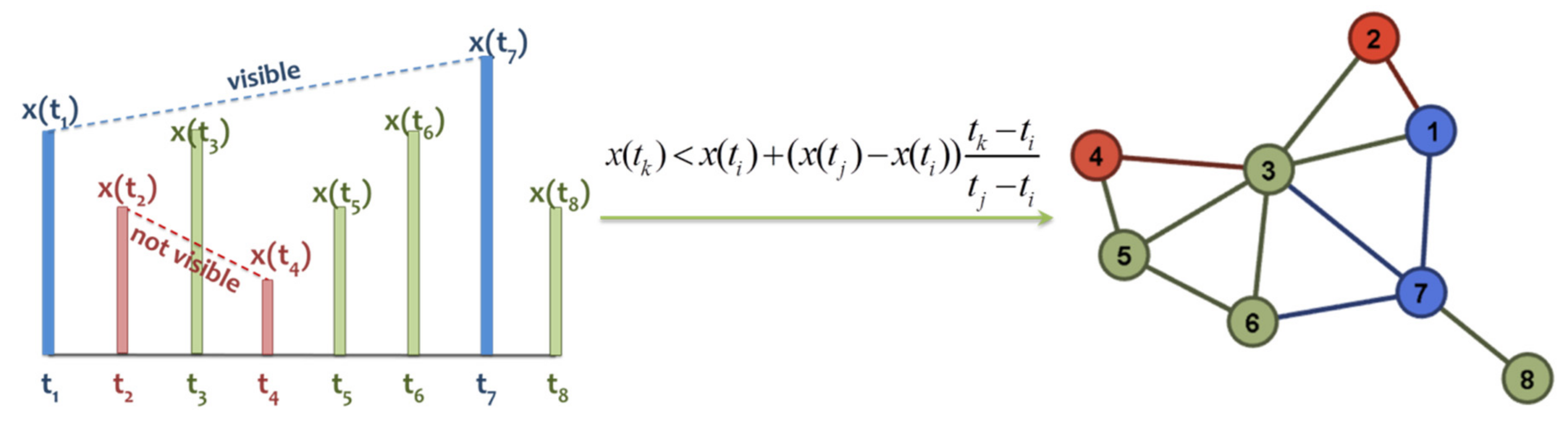
25]. A major contribution in this research field was made by [
24], who proposed an algorithm, named the natural visibility graph algorithm (NVG), based on an optics criterion for transforming a time-series into a graph. The authors showed that their algorithm was sufficient to convert fractal series into scale-free networks, supporting the fact that power-law degree distributions are related to fractality [
24]. Some indicative applications of the complex network analysis of time-series include the work of [
26], who observed that the scale-free property in visibility graphs associated to the time-series of energy dissipation rates corresponds to the self-similarity of the energy dissipation rate series and, also, that the hub-to-hub attraction, which was detected in the network, explains the absence of self-similarity in the series. In the work of [
27], which was conducted on an experimental temperature time-series set extracted from a vertical turbulent jet, the authors observed that the complex network approach allows a more detailed detection of various dynamical regions of the jet-flow in a time-series, which was constructed from a vertical turbulent heated jet. In the work of [
28], the authors observed that the average clustering coefficient of a limited penetrable horizontal visibility graph, which was created from oil–water two-phase flow signals, allows the identification of the typical oil–water flow patterns at different scales. Furthermore, the authors of [
29] showed that the power averaging aggregation operator, which is computed on the associated visibility graph, is more effective than other time-series operators. In the work of [
30], the authors observed that the visibility graph-based approach unveils the key temporal properties of the turbulent time-series and their changes due to positive vertical coordinate movements. In the work of [
31], the authors applied the NVG to convert the prime Greek COVID-19 infection curve into a graph. By using the modularity optimization algorithm, they divided the associated visibility graph into connected communities, which revealed within the time-series body a sequence of different typologies introducing the saturation stage in the evolution of the pandemic, a fact that was verified by the global maximum appearing at the beginning of the saturation stage in terms of Gaussian modeling, and by following observations.
Within the context of converting a time-series into a visibility graph, the graph model associated to the time-series appears to inherit structural properties that are consistent with the fractal-like and self-similarity characteristics of the source time-series [
24,
26] and it can generally include immanent structural information that is related to the configuration of the physical system it represents [
28,
29,
30,
31]. Within this framework, this paper studies the chaotic oscillations and the corresponding phase portrait of an already known semiconductor’s time-series by using the complex network analysis of time-series. This study can also apply to alloys that exhibit the same non-linear behavior, or their electrical properties. The analysis aims to examine the structural properties that are immanent in the graph structure associated to the time-series, and to compare the complex network approach with the already known results of the chaos detection analysis of the time-series. The further purpose of the paper is to address the demand for managing the complexity of semiconductor research, with the interdisciplinary approach of complex network analysis of time-series being already effective in various applications.
The remainder of this paper is organized as follows:
Section 2 describes the methodology and data of the study, building on the natural visibility algorithm that is introduced by [
24] and on the previous study [
7] for detecting quasi-periodic and chaotic self-excited voltage oscillations in a ternary semiconductor.
Section 3 shows the results of the analysis and discusses them in comparison with the available findings of the previous work, and, finally, in
Section 4, conclusions are given.
3. Results and Discussion
The results of computing the network measures of the visibility graph associated with the available voltage oscillation time-series are shown in
Table 2. As can be observed, the associated visibility graph is a connective (i.e., including one component) medium-sized graph consisting of 2672 nodes and 11,066 edges (links). The associated visibility graph is a sparse (not dense) graph, including 0.3% of the possible links that can be developed for the certain number of nodes. The degree of the network nodes ranges within the interval [2,324], with an average degree of 8.283 connections. In terms of accessibility, the average path length of the associated visibility graph is 4.496, implying that, on average, two random nodes are distant to each other by almost 4.5 steps of separation. This value is relatively larger than the expected
average path length described for scale-free networks, which have a “good” hierarchical structure [
19,
38] and according to [
42] are considered as “ultra-small”. This slight deviation from “scale-freeness”, as expressed by the average path length |4.496 − 3.82|/3.82
17.8%, indicates the existence of (relatively loose) spatial constraints [
36], which are obviously related to the chain structure of the source time-series. Further, the network diameter of the visibility graph is 11, expressing that the most distant nodes in the network are a distance of 11 steps of separation away.
Next, the clustering coefficient of the associated visibility graph is 0.772, expressing that a randomly chosen node in the network is 77.2% more likely to have connected neighbors. This value implies a good level of circulation in the information spreading in the network. Finally, the modularity function of the visibility graph is 0.753, implying a good (at the 75% level) tendency of the graph to be divided into communities. In particular, the visibility graph can be divided into 68 communities, which will be further discussed in a following paragraph.
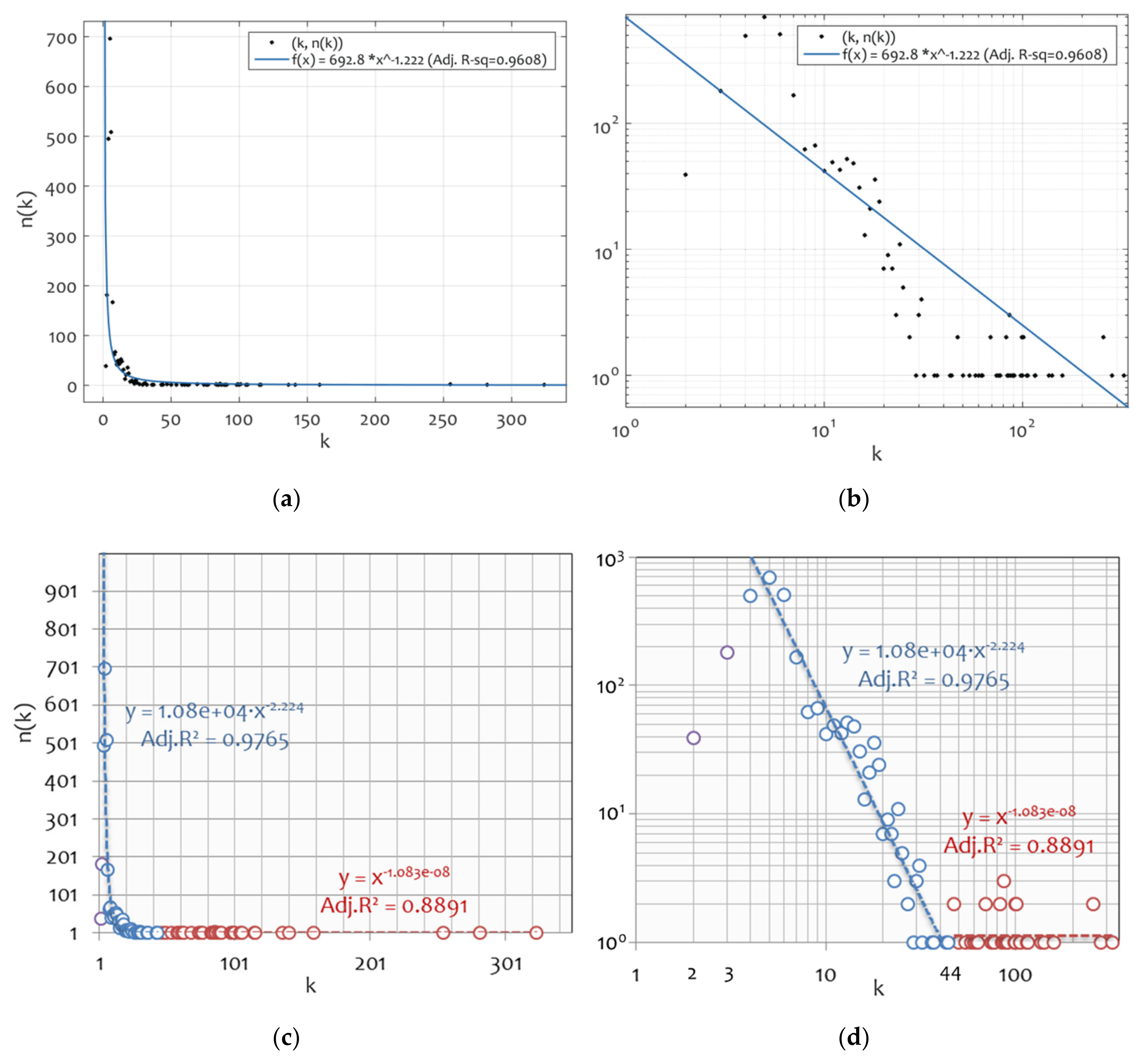
In terms of pattern recognition,
Figure 3 shows the degree distribution of the visibility graph associated with the available voltage oscillation time-series of TlInTe
2, at the metric and log–log scale. As can be observed, the degree distribution fits closely to a power-law pattern (
R2 = 0.9608), which is an indication of scale-freeness according to the definition of the scale-free property [
19,
35]. However, the power-law exponent of the visibility graph
γvis = −1.222 does not lie within the typical scale-free range of [2,4] that describes empirical cases of scale-free networks, a fact that may be related to the effect of spatial constraints observed based on the magnitude of the accessibility network measures (average path length, network diameter) and describes the restriction of the visibility graph in developing distant connections. To get a more detailed picture, power-law fittings with cut-offs (see [
43]) are also applied to the available degree distribution. As can be observed in
Figure 3b,c, the region between degrees
k = 4 and
k = 44 (including 90.23% of the total data) yields the best possible power-law fitting (adjusted
R2 = 0.9765) to the degree-distribution data, and lies within the typical range of scale-freeness describing empirical cases of real-world networks.
On the other hand, the degree distribution in the region of higher degrees (i.e.,
k > 44, including 1.53% of the data), which can be considered the hubs’ region, configures a tail that is almost described by a linear and particularly constant pattern (of the form y ≈ x
−0 = x
0 = 1). This implies that the main body (90.23% of the data) of the TlInTe
2 voltage oscillation visibility graph is satisfactorily described by the scale-free property, a fact that illustrates the chaotic configuration of the TlInTe
2 voltage oscillation time-series within the context of the fact that the visibility algorithm relates the scale-free property with the fractal-like structure of the time-series [
24]. However, the hub region does not seem to exhibit this scale-free property because its degree distribution is described by linearity (constancy). This observation implies that the hub configuration of the TlInTe
2 voltage oscillation visibility graph does not adhere to the “good” structure of hierarchy expressed by the scale-free property, but instead to a constant rule diverting the hierarchical order. Provided that the hubs in this visibility network are greater in number than those expected by a scale-free pattern, the constant configuration of the hub region can imply the effect of spatial constraints to the extent that the network’s ineffectiveness in developing more distant connections leads to the emergence of more hubs.
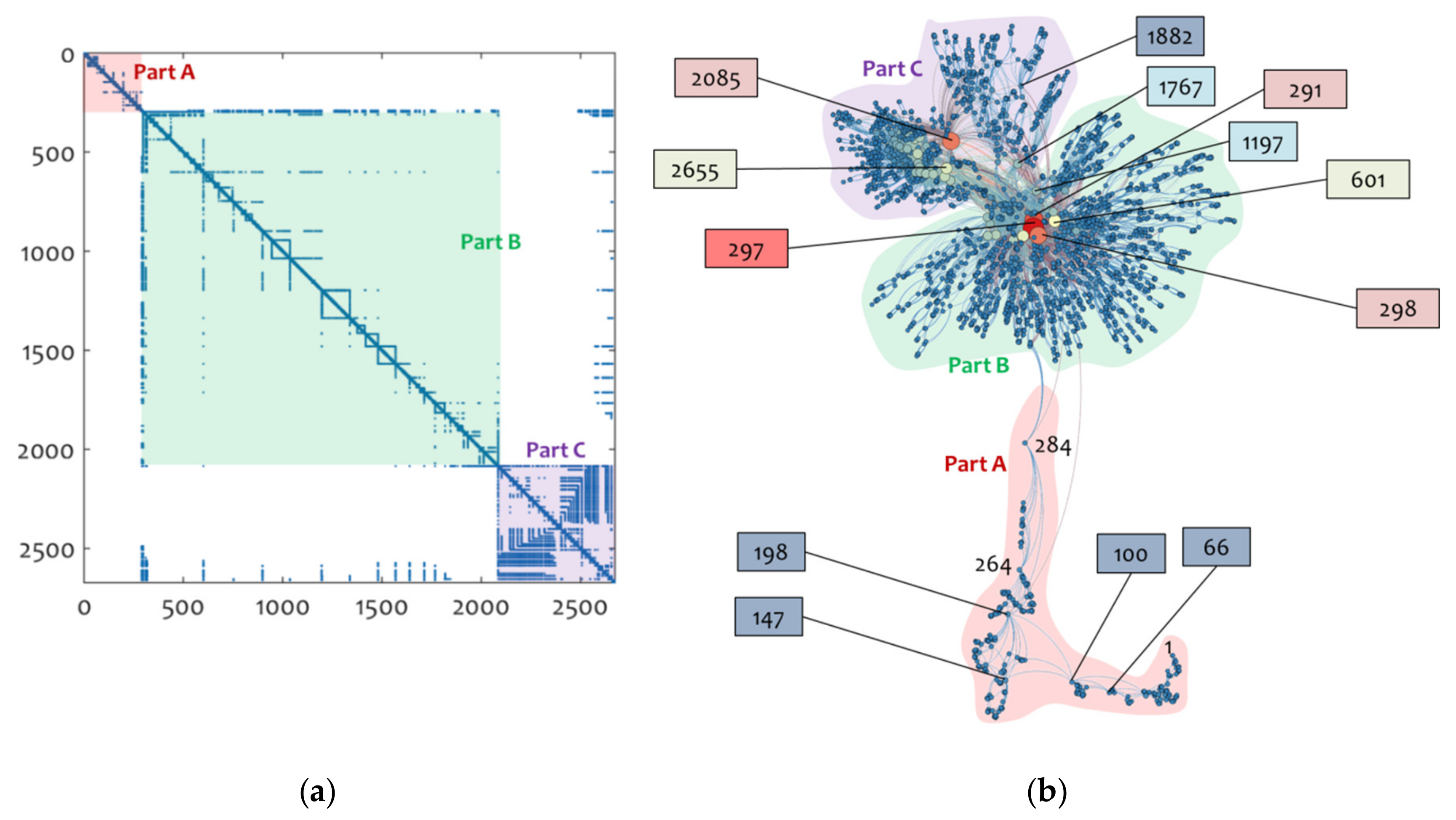
Furthermore,
Figure 4 shows the spy plot and the Force-Atlas graph layout produced using the open-source software of [
44]. Both these diagrams suggest different visualizations of the network topology, with the first illustrating the network embedded in a matrix space and the second in a topological space. In particular, a spy plot is a dot representation of the network’s adjacency matrix, displaying nonzero elements (which express network links) with dots. The spy plot can be insightful for pattern recognition in graphs because it can display connectivity patterns within the adjacency matrix [
38]. On the other hand, the Force-Atlas layout is a 2-dimensional representation provided by the open-source software of [
44] that is generated by a force-directed algorithm (see [
38,
45]) with default parameters. The algorithm applies repulsion strengths between network hubs, while it arranges the hubs’ connections into surrounding clusters. Therefore, the graphs that are shown in this layout have their hubs placed at the center of the plane, but at mutually distant positions, so that their distance can be as great as possible, whereas lower-degree nodes are placed as close as possible to their hubs. Provided that both these layouts represent the network embedded in different spaces (i.e., a matrix and force-directed topological space, respectively), they both illustrate different pictures of network topology in a certain growth timeframe. Within this context, the prediction of network growth based on these layouts is linked to pattern recognition, which is made evident by these layouts, namely to the extent that a certain network topology is theoretically or empirically related to a certain growth process (e.g., a lattice-like topology is related to “linear” network growth, revealing the effect of spatial constraints, a random topology is linked to an irregular growth, and the scale-freeness is connected to the “preferential attachment” growth mechanism). For more details see the suggested literature [
19,
36,
38,
45].
In
Figure 4, first, the spy plot illustrates a major arrangement of connections along the main diagonal, which refers to a typical pattern of lattice-like network topologies [
38,
45]. However, the node region 291–298, along with the node places 601 and 2085, denote some significant connectivity zones in the spy plot, indicating the existence of hubs in the network, which implies that the topology of the visibility graph is more complex than a lattice-like one since it is equipped with hierarchical structures related to the scale-free property, as is captured in the previous degree distribution analysis. Further, the node zones 291–2085 (
Figure 4a, Part B) and 2085–2672 (
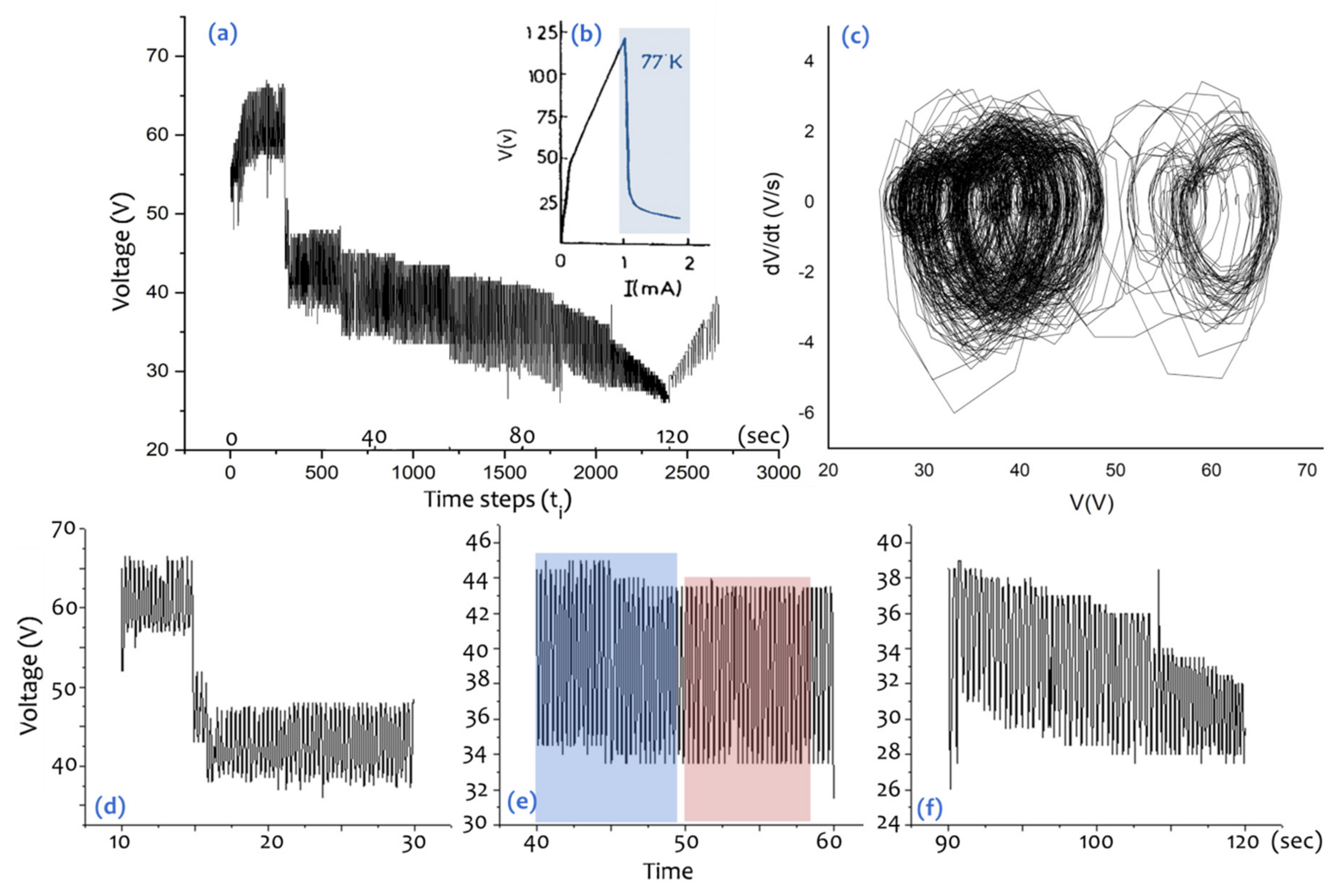
Figure 4a, Part C) illustrate two major square connectivity patterns in the spy plot of the visibility graph, which may correspond to the pair of attractors that are captured in the chaos detection analysis provided by [
7] and are shown in
Figure 1. An intuitive picture of the chaotic structure of the voltage oscillation time-series of TlInTe
2 can be shaped by observing the fractal-like tiling configured within these square connectivity areas (
Figure 4a, Parts B and C).
Next, the network layout of the visibility graph shown in
Figure 4 shows a pattern supporting that of the spy plot. Within this context, the Force-Atlas layout of the visibility graph depicts the two major sub-networks defined by the hub families {291,298,297,601,1197} and {2085,2655}, which correspond to Part B (
Figure 4b) and Part C (
Figure 4b), respectively. This observation adheres to the previous findings of the spy plot examination, and it further supports the linkage between the pair of sub-networks corresponding to Parts B and C (
Figure 4b) and the pair-wise structure of attractors extracted in the analysis of [
7]. On the other hand, the tail that was observed in the graph and that includes the hub-like nodes {66,147,198,264,284} corresponds to Part A of the spy plot shown in
Figure 4a. Overall, the sequential arrangement of Parts A, B, and C, which is observed in both the spy plot and the Force-Atlas layout of
Figure 4, illustrates that the visibility network’s main constraint is in developing distance connections (a condition that is usually expressed as the “spatial constraints” of the network structure, see [
36]), and therefore it supports the finding that the visibility graph associated to TlInTe
2′s voltage oscillations time-series is described by lattice-like characteristics that can be related to the semi-periodic sections of the time-series.
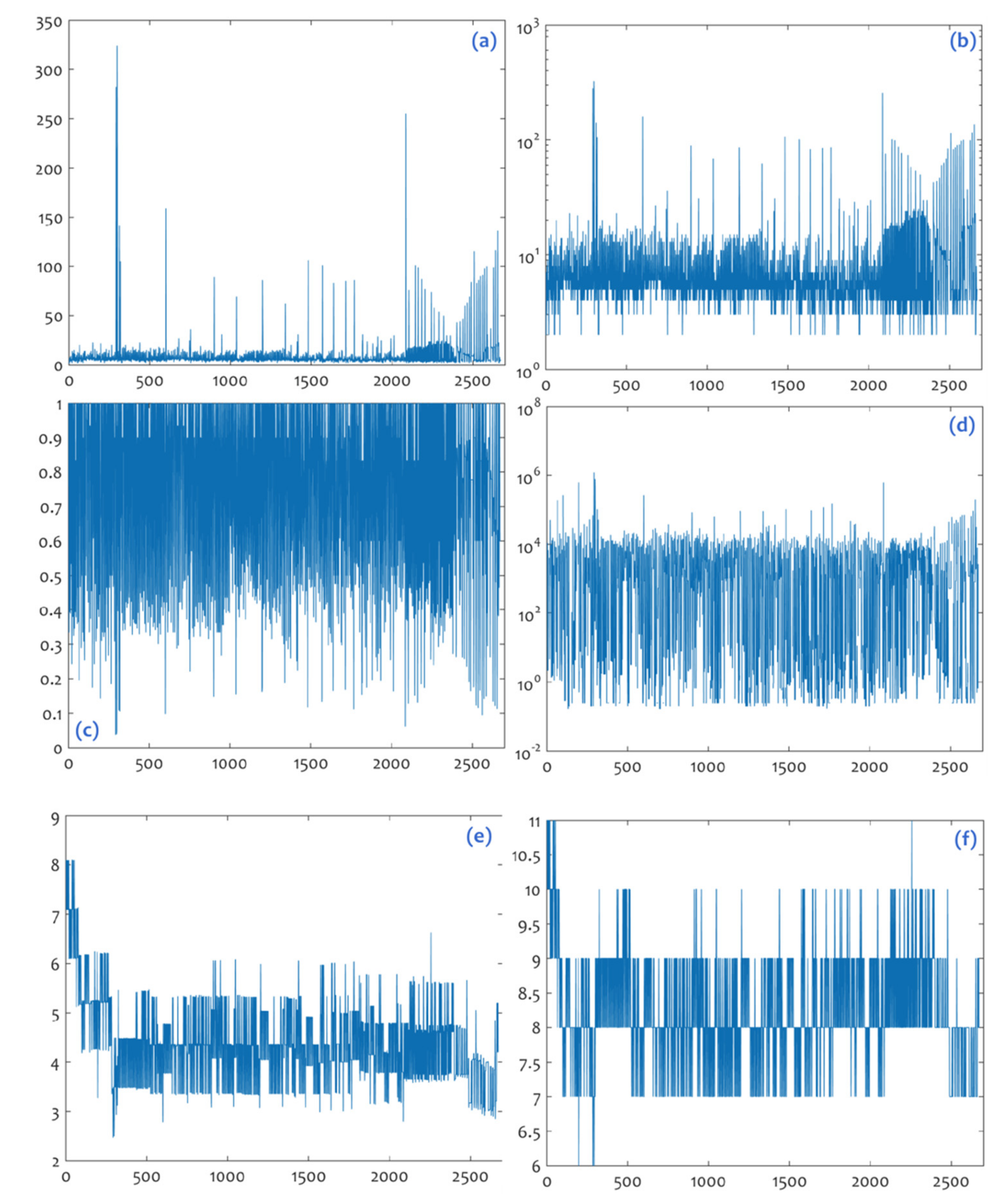
In the final step of network analysis, a set of secondary time-series is created from the visibility graph. These secondary time-series include network measures that are computed for each node of the visibility graph and are arranged into the node ordering of the source (TlInTe
2) time-series. In terms of interpretation, each secondary time-series expresses the score that a node of the source time-series has in its associated visibility graph, for a certain measure. Within this context, the secondary time-series that are computed refer to the network measures of degree, clustering coefficient, betweenness and closeness centrality and eccentricity (i.e., the distance of a node to the center of the network, see [
35]), and they are shown in
Figure 5.
The line diagrams shown in
Figure 5a,b illustrate the time-series node ordering of the connectivity hubs in the visibility graph, and are insightful in discriminating the hub families composed of nodes {291,298,297,601} and {2085,2655}, which were previously observed. The two next diagrams of clustering coefficient (
Figure 5c) and betweenness centrality (
Figure 5d) are perhaps not so insightful in terms of zone detection, but through a careful consideration, they seem to support the central roles of the nodes 291, 298, 297, 601, 2085, and 2655. A cleared picture of the hub-grouping is offered by the diagrams of closeness centrality (
Figure 5e) and eccentricity (
Figure 5f). However, a clearer observation about these diagrams regards their fractal-like tiling structure, which complies with the chaotic behavior of the voltage oscillation time-series of TlInTe
2. This observation can configure the research hypothesis that the accessibility-defined measures of the visibility graph can preserve the chaotic characteristics of the source time-series, suggesting a topic of further research.
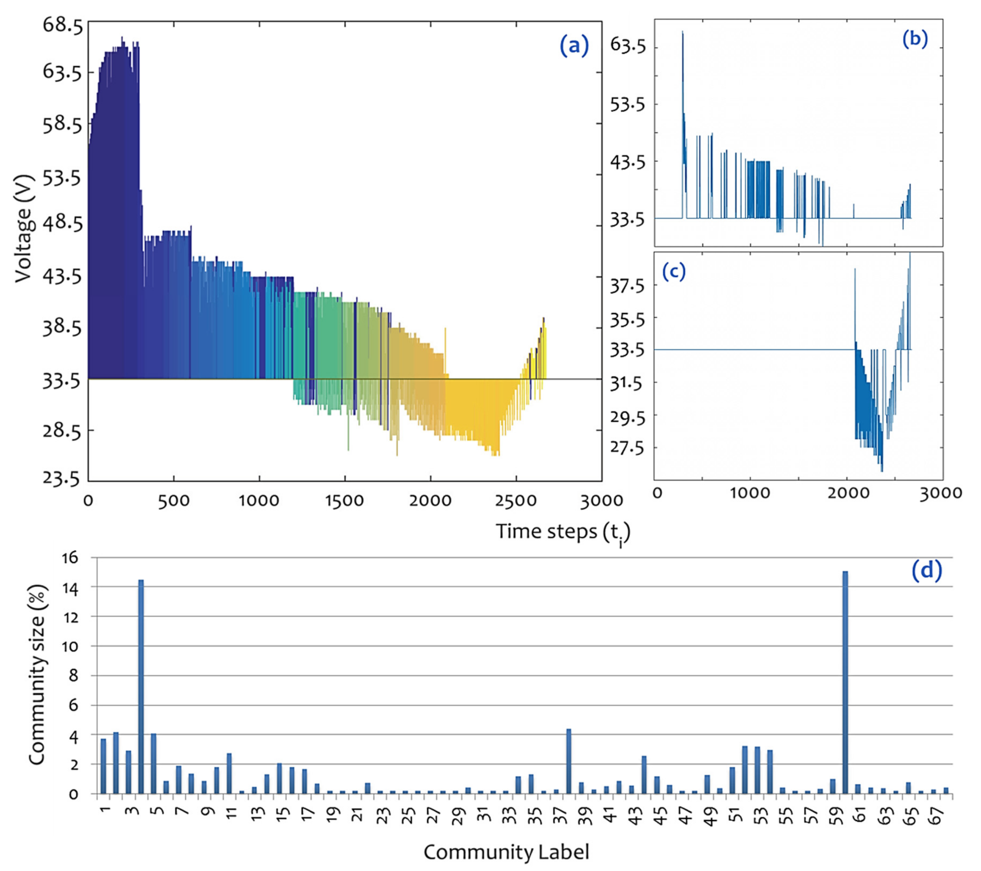
In the final step of analysis, the associated visibility graph is divided into connected communities by using the modularity optimization algorithm of [
39]. The analysis results in 68 communities, as is shown in
Table 2 and (in more detail) in
Figure 6. As can be observed in
Figure 6a, the majority of communities include successive nodes, except from the cases of community
Q4 (
Figure 6b) and
Q60 (
Figure 6c), which are the two major communities, each containing over 14% of the total time-series nodes. In particular, community
Q4 includes 388 nodes that are placed in positions from 291 to 2661, and community
Q60 includes 403 nodes that are placed in positions from 2085 to 2655. In terms of physical interpretation, the structure of community
Q4 is indicative of the voltage decay that describes the total behavior of the available voltage oscillation time-series of TlInTe
2, whereas the structure of community
Q5 includes the characteristic voltage sink recorded in the timeframe from 100 up to 138 s (
Figure 1).
According to
Figure 6d, the majority of communities include individually less than 2% of the total time-series nodes, and only 12 out of 68 communities, namely
Q1 (3.74%),
Q2 (4.19%),
Q3 (2.92%),
Q4 (14.52%),
Q5 (4.08%),
Q11 (2.77%),
Q15 (2.10%),
Q38 (4.42%),
Q52 (3.26%),
Q53 (3.22%),
Q54 (2.99%), and
Q60 (15.08%), include over 2% of the total time-series nodes. As already mentioned, 66 out of 68 communities consist of successive (i.e., of the form
tk,
tk+1, where
k is a positive integer) nodes, except from cases
Q4 and
Q60, which also include intermediate gaps. The positioning and the major successive configuration of the communities composing the available voltage oscillation time-series of TlInTe
2 imply that this time-series is majorly described by spatial constraints, which are captured by the lattice-like node arrangement along the main diagonal in the spy plot, as well as by the tailed node arrangement shown in the Force-Atlas layout in
Figure 4. However, the emergence of two major communities in the visibility graph that exceed the typical sequential structure describing all other communities is related to parts of superior structural behavior in the time-series. This case of unconventional communities complies with the scale-freeness detected in the network analysis shown in
Figure 3 and
Figure 4, with the chaotic behavior of the source time-series (TlInTe
2) that is the default research hypothesis for this paper, according to the work of [
7].
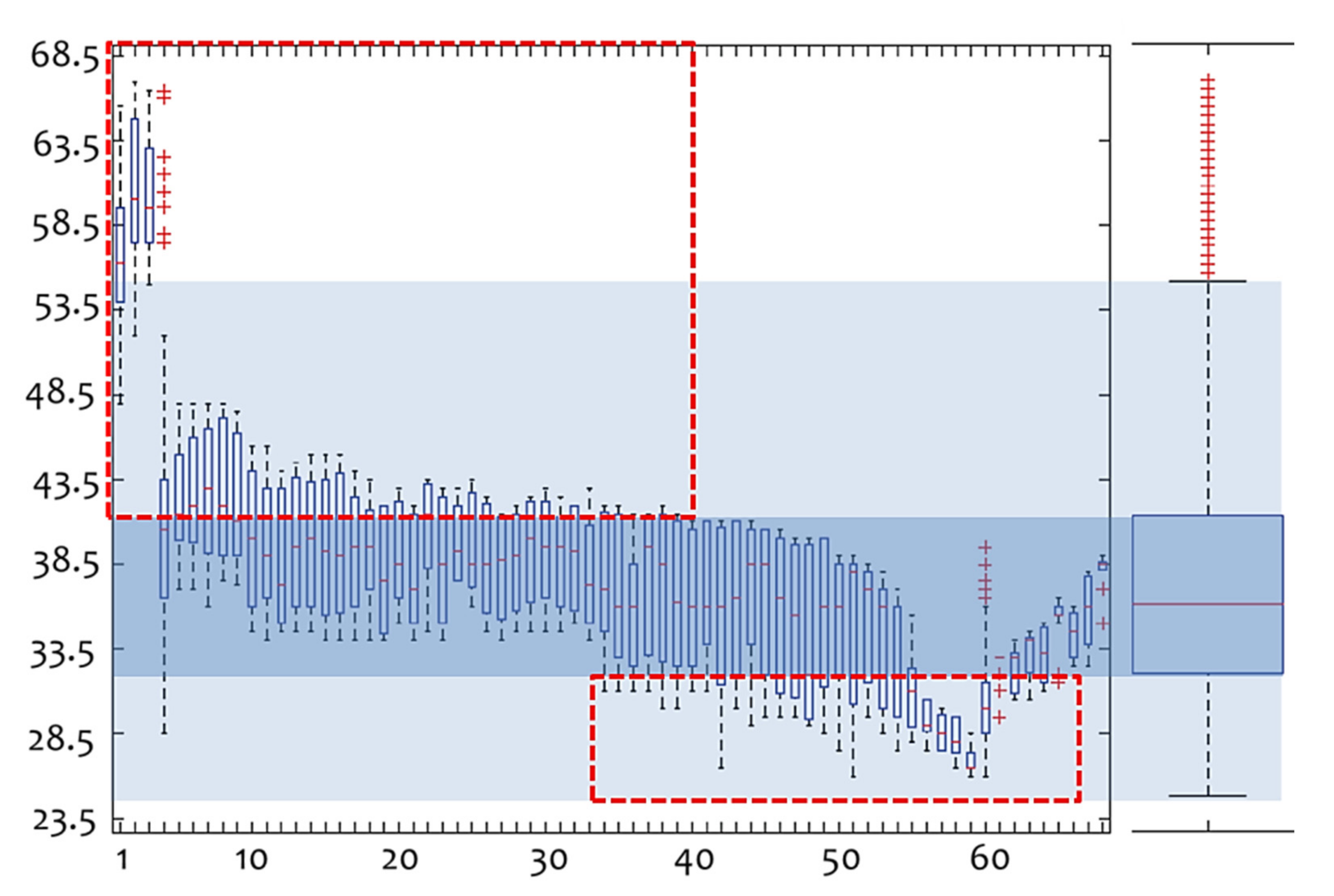
The pair-wise structure expressed by the division of the source time-series into a pair of major communities
Q4 and
Q60 can also be supported by the examination of the voltage values within the 68 available communities. In particular,
Figure 7 shows an arrangement of the box-plots expressing the voltage value distributions within each community, ordered according to the community labeling. As can be observed, there are two areas exceeding the interquartile range of the box-plot distribution of the available communities in
Figure 7. These areas include non-typical voltage values of the voltage oscillation time-series of TlInTe
2, to the extent that these values exceed 50% of the cases around the mean and lie at the edges (in a two-tailed configuration) of the voltage distribution of TlInTe
2. This result also complies with the previous findings, and can further support the chaotic structure expressed by the pair of attractors configured in the phase portrait of voltage oscillations that is shown in
Figure 1.


