1. Introduction
In quantum electrodynamics (QED) the vacuum is a dynamical entity, in the sense that there are a rich variety of processes that can take place in it [
1,
2,
3]. There are several observable effects that manifest themselves when the vacuum is perturbed in specific ways: vacuum fluctuations lead to shifts in the energy level of atoms (Lamb shift) [
4], changes in the boundary conditions produce particles (dynamical Casimir effect) [
5], and accelerated motion and gravitation can create thermal radiation (Unruh [
6] and Hawking [
7] effects).
Free quantum field theories predict the existence of vacuum fluctuations, which are particle-antiparticle pairs that appear spontaneously, violating the conservation of energy according to the Heisenberg uncertainty principle. These fluctuations play a role in the value of the permittivity of the vacuum
: a photon will interact with those pairs much as it would with atoms or molecules in a dielectric. This idea can be traced back to the time-honored works of Furry and Oppenheimer [
8], Weisskopf and Pauli [
9,
10] and Dicke [
11], who contemplated the prospect of treating the vacuum as a medium with electric and magnetic polarizability.
Such a medium may well consist of particle-antiparticle bound states, as first discussed by Ruark [
12] and further elaborated by Wheeler [
13]. This approach has been recently adopted [
14,
15,
16] to obtain expressions for the permittivity, leading to ab initio calculations of the value of
and to useful discussions of the significance of those calculations [
17,
18,
19,
20,
21,
22]. The main assumption in Refs. [
14,
15,
16] is to represent the bound states by an effective spring constant, which is taken as the frequency corresponding to an energy
(
c being the speed of light); that is, twice the rest mass
m of the pair. On the other hand, Mainland and Mulligan [
23,
24,
25] do relate the binding energy of the particle-antiparticle pair to the lowest level of a harmonic oscillator, to give what might be considered to be a true oscillator model.
In the standard relation , linking the electric displacement vector and the electric field vector , the first term on the right-hand side is often referred to as the polarization of the bare vacuum. In QED, however, the polarization due to vacuum fluctuations is added as part of . Because the new term is dispersionless (like ), the electric field can be rescaled to formally recover the initial equation. We suggest that the polarization of the vacuum fluctuations should instead be identified with the first term . This is a paradigm shift in our physical picture of the vacuum. One consequence of this is that in a really bare vacuum, in absence of vacuum fluctuations, the speed of light becomes undefined. Nonetheless, this is only an academic consideration without practical relevance.
We will show here that this interpretation of
is consistent with QED. The vacuum has a crucial property that it does not share with dielectric and magnetic materials: it is Lorentz invariant. Due to this property Michelson and Morley failed to detect the motion of the Earth through the "ether", which, in the present context, is the quantum vacuum [
26]. Empty spacetime is homogeneous, so variations of the permittivitty
and permeability
can occur only in the presence of charged matter. The linear response of vacuum must be Lorentz invariant, so in reciprocal space the susceptibility of vacuum must be a function of
, where
is the photon frequency and
its wave vector. The condition
, describing a freely propagating photon, is referred to as on-shellness in QED: a real on-shell photon verifies then
.
This paper is organized as follows.
Section 2 describes vacuum polarization due to creation of virtual particle-antiparticle pairs in the framework of QED. In
Section 3, we show how a mass-independent response model can be derived from the results in QED and how
can be indeed interpreted as vacuum polarization. As stressed before, this is a major change in our understanding of the vacuum: as the off-shellness rises, the charge
e is held constant, while only
is allowed to change. This is in sharp contrast with standard models, such as the one proposed by Gottfried and Weisskopf [
27], which is explored in
Section 4. Finally, our conclusions are summarized in
Section 5.
2. Vacuum Polarization in QED
As heralded in the Introduction, the vacuum in QED acts as if it were a dielectric medium where the virtual pairs shield the original point charges. In this Section, the vacuum contribution to the dielectric permittivity
will be calculated by incorporating it into the electromagnetic Lagrangian. In QED the bare potentials
and charge
are rescaled by a constant factor
to give the physical four-potential
and the physical electron charge
e; that is [
28],
This rescaling is at the basis of the renormalization program. The renormalized QED Lagrangian density will be written as
where,
describes the electromagnetic free field,
accounts for the Dirac field (details are omitted because renormalization of the masses will not be discussed here) and the interaction term
is
Here,
is the current due to real charges, while the current density
due to the creation of virtual pairs and the
counterterm are incorporated into
. Together, they describe the reduction in vacuum polarization relative to its maximum value at
. The current induced in the vacuum by the four-potential
due to virtual pairs of type
(where
corresponds to the possible different leptons) is
where
is the metric tensor, with diagonal
, and
is the QED vacuum polarization of a
-type particle. If
describes real photons, the on-shell condition
is satisfied. This is a generalization of the usual textbook treatment of electron-position virtual pairs [
28,
29], extended to other fermions.
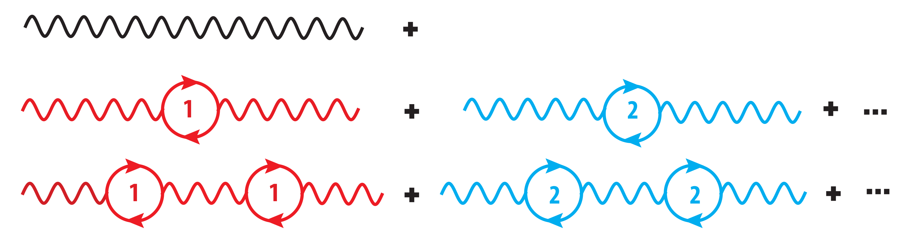
The Feynman diagram in
Figure 1 is a pictorial representation of vacuum polarization in the one-loop approximation. The wavy lines represent an electromagnetic field, while a vertex represents the interaction of the field with the fermions, which are represented by the internal lines. The loop labeled 1 corresponds to a virtual electron-positron pair, the loop 2 the creation of a muon-antimuon pair, and so on. The total vacuum polarization can then be jotted down as
Henceforth, the sum in is over all elementary charged particles (e. p.). We stress that vacuum fluctuations are on-shell once they appear. However, vacuum polarization is a matter of virtual particles that occur off-shell as part of a perturbative calculation.
In the on-shell counterterm [
29]
where
is the leading order approximation to
, which is the one depicted in the second row of
Figure 1.
The vacuum polarization
) is a divergent sum over fermion momenta and naive introduction of a cut-off leads to a physically unreasonable result: the photon mass is infinite [
28,
30]. Since observations are made near
, the change of vacuum polarization relative to its on-shell value,
is the relevant quantity. Writing
as
to separate it into fully polarized and polarization-reduction terms and integrating
by parts to get its (
form [
29], the Maxwell Lagrangian density becomes
where
B is the magnetic field flux density, and
and we have used
. For most practical purposes, in (
9) we can replace
by its second-order approximation
, which reads [
29]
where
ℏ is the Planck constant and
. The equation in the second line is valid when
.
The function
can be continued in the complex
plane. This yields a dispersion relation linking the real and imaginary parts of this polarization tensor. A lengthy calculation shows that [
28]
which gives the absorptive part, independently of any regularizing cutoff. Note, however, that this absorption only happens
, which corresponds to the process of pair creation in an electric field.
In classical electromagnetism
. This relationship is maintained here except that, with running,
. The linear response of the vacuum is then described in reciprocal
k space by
where
H is the magnetic field strength.
The Maxwell equations in vacuum can be derived from the Lagrangian (
2), following the standard method. They take the usual form in
k-space:
The photon two-point correlation function is found by solving (
4) for
[
29]. Using Equation (
9), it can be written as
This
is the response to a
-function source in real space and hence to a constant driving force in
k-space. Equation (
14) is then a Green function satisfying Maxwell’s wave equation. In the Lorenz gauge, and in
k-space this is
where
is
k independent. The matter-field coupling constant is
Since
contains all powers of
, it incorporates summation over all numbers of pairs as sketched in
Figure 1 and used in the calculation of (
14). When restricted to an energy scale
, the sum is over all fermions of mass less than
[
31,
32,
33].
Note that, according to (
16), the coupling constant runs with
. However,
contains both the charge
e and the permittivity
. It is usual to keep
fixed, and let
e run, as in the Gottfried-Weisskopf model we shall examine in
Section 4. The present paper keeps
e fixed, and lets
run. This is in most ways equivalent to running the effective charge, but the physical interpretation is different. In a dielectric it is possible to have
but
makes no physical sense.
The dielectric properties of vacuum differ from those of a material medium in two important ways:
dependence replaces the usual
dependence and Lorentz invariance requires that
. Lorentz invariance is not only a symmetry of the laws of physics, but also of the quantum vacuum. Actually, the principle of relativity of uniform motion can be identified with the Lorentz invariance of Maxwell equations [
34]. The speed
c is a universal constant (Interestingly, even without imposing this requirement and when using the dielectric model in the next section to independently calculate
, the resulting speed of light is independent of how many types of elementary particles contribute, as long as there is at least one type, and agrees with the limiting speed in Lorentz’s equations [
15]), whereas the coupling constant
runs. On the photon mass shell
, so a free photon always sees
and there is no running. Both the polarization
and the magnetization
are nonzero; however,
as it must for propagation in free space. A free electromagnetic wave polarizes and magnetizes the vacuum but the polarization current exactly cancels the magnetization current (This bears some resemblance with the interference between the emitted electric and magnetic dipole waves leading to forward scattering only and no back scattering, the property of Huygens waves which typically appear in materials with comparably strong electric and magnetic interaction, which holds for the vacuum [
35] and was recently rediscovered for metamaterials [
36].).
3. Connection with a Dielectric Model
An individual loop in
Figure 1 is analogous to a single polarizable atom with center of mass momentum
. If, for simplicity, we set
, the computation of the Feynmann diagrams involve integrals of the form
, which entail an exponential decay,
, in real space. Therefore, the "radius" of a virtual atom is of order
. All in all, this suggests that one might model the particle-antiparticle vacuum fluctuations as two-level atoms with level spacing
and occupying a volume of the order of
.
When a virtual pair is created from a photon of frequency
[
37] its excess energy is, according the Heisenberg uncertainty principle,
, so it can exist only for a time
. (While a real pair cannot be created by absorbing a photon due to simultaneous conservation of energy and momentum, this restriction does not apply to the ephemeral creation of virtual pairs.)
Based on the uncertainty principle and this simple dielectric model, one can readily find that the permittivity of vacuum can be expressed as [
14,
15]
where
f is a geometrical factor of order unity,
is charge and the sum is over all elementary charged particles.
This is consistent with QED, as discussed in the previous Section. Indeed, at large
and to second order in perturbation theory as in Equation (
10), we have that
We know that at high momentum (or energy) scale, the coupling constant
in QED becomes infinity [
38,
39]. If
is the value of that momentum (which is usually called the Landau pole [
40]), then
and hence the fudge factor
f in the dielectric model is given by
For the standard model and with two additional charged Higgs particles of eV, and all of is vacuum polarization if .
If running is neglected, the on-shell Maxwell equations in a medium with charges and current sources are
as in classical electromagnetic theory. Equation (
21) allow us to define the four-vector potential that drives the creation of the pairs. Equation (22) simply say that charge density is the divergence of polarization and the current is the sum of its polarization and magnetization parts.
Our results support the conclusion of Zeldovich, who considered a Lagrangian in which all of the electromagnetic term comes from the interaction of the particle with the field and came to an interesting interpretation [
41]: in the absence of vacuum polarization, electric and magnetic fields act on Dirac fermions, but there is no field energy and no electromagnetic wave propagation. In an absolute void it makes no sense to talk about Maxwell’s equations or light propagation. In QED, the connection between vacuum fluctuations and field propagation ensures that the electromagnetic vacuum also satisfies invariance under Lorentz transformations [
42]. Only after vacuum polarization is introduced does the effective Lagrangian give Maxwell’s equations, electromagnetic waves travelling at the speed of light and photons.
Since our dielectric model is compatible with QED, one would expect the same kind of dispersion relations. Therefore, as discussed before, the absorptive behavior only appears at momenta .
4. Gottfried-Weisskopf Dielectric Model
Gottfried and Weisskopf [
27] introduced a toy model to understand the physical mechanisms involved in vacuum polarization. In this simple picture, one assumes that the bare charge
is uniformly distributed in a small sphere of radius
a [
]. When this charge distribution is surrounded by a spherical shell of inner radius
, filled with a dielectric medium permittivity
, an induced charge of opposite sign appears on the inner surface of the shell at radius
r, canceling part of the charge
for an observer at a distance larger than
r. Obviously, at the outer surface of the dielectric medium, an equal charge of opposite sign appears. However, if the charge is measured from within the medium it will appear to be reduced, precisely by the permittivity
[
43].
When one considers the vacuum, one has to take into account that it extends to infinity. Now, the permittivity depends on the distance r to the charge. This is so because at r only those virtual pairs having Compton wavelengths contribute. We can interpret this model from a QED viewpoint. To this end, we define the relationship between and at charge separations where the coupling strength can be measured; that is, at large distances or, equivalently, small momenta, where the vacuum is maximally polarized. With polarization included the dielectric permittivity is at the physical scale. In consequence, is the reduction in polarization.
Since
is not a constant, the exact relationship between
and
is nonlocal in
r-space. It is not, in general, correct to write the potential as
. The simplest example in which running coupling can be expressed as an explicit local function of
r is a static charge, say
In the Coulomb gauge
and
. Equation (
13), with
, then gives
which in
-space reads
equivalent to Equation (7.93) in [
29].
For electron-positron pairs alone the magnitude of
is very much less that 1 so that
is approximately
and [
44]
where
α is the fine structure constant,
is the mass of the electron,
r is the distance from the fixed charge and
is Euler’s constant. The dielectric constant
decreases with increasing
or decreasing
For
the Coulomb interaction becomes stronger as the charges approach each other.

