Hybrid Machine Learning-Based Approaches for Feature and Overfitting Reduction to Model Intrusion Patterns

Abstract

An intrusion detection system (IDS), whether as a device or software-based agent, plays a significant role in networks and systems security by continuously monitoring traffic behaviour to detect malicious activities. The literature includes IDSs that leverage models trained to detect known attack behaviours. However, such models suffer from low accuracy or high overfitting. This work aims to enhance the performance of the IDS by making a model based on the observed traffic via applying different single and ensemble classifiers and lowering the classifier’s overfitting on a reduced set of features. We implement various feature reduction techniques, including Linear Regression, LASSO, Random Forest, Boruta, and autoencoders on the CSE-CIC-IDS2018 dataset to provide a training set for classifiers, including Decision Tree, Naïve Bayes, neural networks, Random Forest, and XGBoost. Our experiments show that the Decision Tree classifier on autoencoders-based reduced sets of features yields the lowest overfitting among other combinations.

1. Introduction

Intrusion detection systems (IDSs) represent proactive defence mechanisms that leverage advanced data analytics to identify malicious activity, suspicious behaviour, abnormal patterns, policy violations, and security breaches within a network domain or a host system. The escalating adoption of diverse network devices has increased systems’ vulnerability, making them more susceptible to exploitation by hackers to compromise the CIA triad [1] in terms of targeting the Confidentiality, Integrity, and Availability of the systems. The two main categories of intrusion detection in an IDS are: (1) anomaly detection, which involves detecting deviations from normal behaviour; and (2) misuse detection, which involves detecting known malicious patterns.

The IDS, however, suffers from a number of deficiencies, including:

• Low accuracy, high false positive rate, or high amount of model’s overfitting [2,3,4,5].
• Inefficiency in dealing with big data, which is common in network attacks [2,6,7].
• Keeping a stable detection rate when different volumes of traffic and types of intrusion are encountered [6].
• Incapability to detect unknown zero-day attacks [6].

In this work, we focus on enhancing the performance of the IDS by reducing overfitting and increasing the accuracy of the classification models using hybrid machine learning-based approaches. To assess the efficacy of our detection mechanism, we conducted a controlled experiment on a real-world network traffic dataset. Our main research question is whether hybrid machine learning-based approaches can enhance intrusion detection accuracy by reducing network traffic features and the overfitting of the model.

Some of the major benchmarking IDS datasets that are often utilized in research are KDD’99 [8], NSL-KDD [9] (an improved version of the KDD99), CIC-IDS2017 [10], and CSE-CIC-IDS2018 [11]. The KDD99 dataset has four types of intrusion categories: DOS (Denial of Service attack), R2L (Remote to Local attack), U2R (User to Root attack), and Probe. The CSE-CIC-IDS (The Communications Security Establishment (CSE) and the Canadian Institute for Cybersecurity (CIC)) 2018 dataset [11] includes seven types of attacks, including Brute-force, Botnet, DoS, DDoS, Heartbleed, Web attacks, and infiltration of the network from inside. The sub-attack types for KDD99 and CSE-CIC-IDS2018 are presented in

Table 1. Attack categories and types in the KDD99 dataset [8].

Attack Category	Sub-Attack Types
Probe	Portsweep, IPsweep, Nmap, Satan
DoS	Neptune, Smurf, Pod, Teardrop, Land
U2R	BuferOverfow, LoadModule, Perl, Rootkit
R2L	GuessPassword, FtpWrite, Imap, Phf, Multihop, Warezmaster, Warezclient

and

Table 2. Attack categories and types in the CSE-CIC-IDS2018 dataset [11].

Attack Category	Sub-Attack Types
Brute-force	Brute-force-Web, Brute-force XSS, FTP Brute-force, SSH Brute-force
Botnet	Zeus, Ares
DoS	DoS-Hulk, DoS-SlowHTTPTest, DoS-Slowloris, DoS-GoldenEye
DDoS	DDoS-HOIC, DDoS-LOIC-UDP, DDoS-LOIC-HTTP
Web attacks	SQL Injection, Command Injection, Unrestricted File Upload
Heartbleed	Heartleech
Infiltration

.

Contributions: We perform three phases of data preprocessing, feature selection and reduction, and attack detection to find the best combination of machine learning approaches. We select the CSE-CIC-IDS2018 dataset [11] for our experiment since it has more recent attack patterns. All implementation and experiments are performed using R studio. We implement various feature reduction approaches, including Boruta, Random Forest, LASSO, and deep learning-based methods, and executed them on the CSE-CIC-IDS2018 dataset. We investigate the issue of model overfitting by utilizing different single models and ensemble classifiers such as LASSO, XGBoost, and dropout mechanisms in deep neural networks to combat overfitting. We demonstrate the effectiveness of Decision Tree classifier with the least amount of overfitting on the reduced sets constructed from autoencoders.

Outline: The rest of this paper is organized as follows. Section 2 reviews the related work. Section 3 describes materials and methods for conducting this research. Section 4 provides the results of our experiments. Section 5 discusses our findings. Finally, Section 6 draws conclusions and future works.

2. Related Work

Khan et al. [2] used the KDD99 dataset and employed a convolutional neural network (CNN) technique to capture impactful features and propose a robust classification. CNN is a feed-forward multi-layered neural network consisting of multiple pooling and fully connected (dense) and convolution layers. Their CNN architecture for feature extraction has three hidden layers, each using a convolutional layer and a pooling layer, and used a softmax classifier.

Laghrissi et al. [7] employed three models of Long Short-Term Memory (LSTM), which is a recursive neural network (RNN) that remembers some context and forgets the rest. The main applications of LSTM are grammar learning, speech recognition, time-series prediction, and sentiment analysis. They used LSTM-PCA (Principal Component Analysis), and LSTM-MI (Mutual Information) to reduce the dimension, feature selection, and attack detection. They used the KDD99 dataset, and considered multi-class and binary classification problems. Their results show that LSTM-PCA outperforms CNN [2], LSTM-RNN, and pruning VELM [12]. The phases include data preprocessing, multi-class classifications, PCA, and score calculation for MI to achieve the statistical dependencies between two variables.

Shapoorifard and Shamsinejad [3] used the NSL-KDD dataset for their experiments and incorporated K-Means clustering to improve the K-Nearest Neighborhood (KNN) classifiers. They used five clusters equal to the number of attack types and applied KNN to capture the distance of each data to cluster centers based on Euclidean distance. In their approach, they consider both the nearest and the farthest distance (KFN) to form a distance-based IDS. Their framework with K-Means, KNN, and KFN successfully reduced the false alarm and increased the accuracy.

Chkirbene et al. [4] proposed a trust-based intrusion detection and classification system (TIDCS) and an accelerated version of that using NSL-KDD and UNSW datasets. They assumed the trustworthiness reduction in each network node after each attack detection when the node is involved. As a result, a dynamic system cleaning is conducted. The results indicated the ability of both systems to reduce the false alarm rate and improve accuracy.

Li et al. [6] proposed a framework that performs feature selection and grouping by employing the Random Forest technique to build a training set and uses an autoencoder for prediction. Autoencoders are deep neural structures that map the input to the same size of output via encoder and decoder sections, and are used for dimension reduction. Their feature grouping phase includes grouping the features according to their similarity based on the Affinity Propagation clustering algorithm. The anomaly detection phase includes several autoencoders equal to the number of feature subsets. Root-Mean-Squared Error (RMSE) is used to distinguish the normal traffic from the abnormal ones. They used CSE-CIC-IDS 2018 in their experiments and showed that their work is more efficient than [13].

Basnet et al. [14] employed various deep learning frameworks such as Theano, TensorFlow, and fast.ai in detecting attacks based on CSE-CIC-IDS2018 dataset. They showed that fast.ai running on GPU outperformed the other two frameworks with about 99% accuracy and low false positive and negative rates in both detecting and classifying different intrusion types.

Catillo et al. [15] focused on the anomaly detection upon employing a deep Autoencoder on CIC-IDS2017 and CSE-CIC-IDS2018. They aimed to reduce the IDS false alarm and proposed an anomaly detector without the use of GPU accelerators.

D’hooge et al. [16] conducted research to distinguish multiple attack classes using CIC-IDS2017 and CSE-CIC-IDS2018. They utilized a pipeline, including twelve supervised algorithms, and reported that DoS/SSL and botnet classes could be well classified using multiple approaches. They concluded the performance of tree-based classifiers as the best, such that single decision trees recognized DoS, DDoS, and botnet traffic. Decision tree-based methods and, in particular, XGBoost are applicable to six of the seven attack classes.

Fihlo et al. [17] detect the DOS/DDOS attack and its variations, including TCP flood, UDP flood, HTTP flood, and HTTP slow on CIC-IDS2017 and CSE-CIC-IDS2018 datasets by employing Random Forest.

Karatas et al. [18] worked on the CSE-CIC-IDS2018 dataset and focused on the reduction in the imbalance nature of the attack classes. They implemented a synthetic data generation model that generates data for minor classes. Their modelling approach includes KNN, Random Forest, Gradient Boosting, AdaBoost, Decision Tree, and Linear Discriminant Analysis algorithms.

Kim et al. [19] worked on DOS category attacks on both datasets of KDD99 and CSE-CIC-IDS2018 and developed an optimized CNN to detect the DOS attacks. They compared the performance of these classifiers with RNN and reported a better performance for CNN over RNN.

Leevy and Khoshgoftaar [5] surveyed intrusion detection models based on CSE-CIC-IDS2018 dataset until 2020. They studied different approaches such as CNN, deep autoencoders, LSTM, AdaBoost, Random Forest, Decision Tree, and XGBoost. They reported high accuracy in some experiments but mostly suffered from overfitting. They also mentioned the lack of attention in addressing the class imbalance problem.

3. Materials and Methods

Our implementation and experiments were performed in R studio. We downloaded the CSE-CIC-IDS2018 dataset from the Kaggle website [20] with 16,000,000 instances collected over the course of ten days. The attacking infrastructure includes 50 machines, and the victim’s organization has 5 departments, which include 420 machines and 30 servers. This dataset is the result of a collaborative project between the Communications Security Establishment (CSE) and The Canadian Institute for Cybersecurity (CIC) that use the notion of profiles to generate cybersecurity dataset in a systematic manner.

The dataset has several attack profiles in different categories: Botnet, DoS/DDoS, Brute force, Web attack, and Infiltration. There are 80 features in this dataset that are extracted from network traffic using the CICFlowMeter tool. The most important columns within this dataset are: Destination Port, Protocol, Flow Duration, Total Forward Packets, Total Backward Packets, and Label. The Label is the dependent variable which indicates if the flow is benign or attack; the category of attack is mentioned as a label in case of attack.

In our experiments, samples are selected from 6 days of the dataset using a stratified sampling technique. Stratified sampling is a sampling technique to ensure that a representative sample is obtained from a population with diverse subgroups to reduce the potential sampling bias. In our dataset, each subgroup is a collection of tuples with one type of attack vector. As a result, according to

Table 3. Frequency of label values in training and test set using a stratified sampling from CSE-CIC-IDS2018 dataset [11] that we used in our experiments.

Label	Training Set	Test Set
Benign	29,605	10,128
DDOS attack-HOIC	6501	2167
DOS attacks-Hulk	4401	1467
Bot	2434	900
FTP-BruteForce	1801	600
SSH-BruteForce	1801	600
Infilteration	1701	564
DOS attacks-SlowHTTPTest	1301	434
Total	49,545	16,860

, we have 8 subgroups. In our sampling attempt, we kept the percentage of each subgroup to the total number of tuples. For example, the attack vector of Infiltration has 1701 number of samples out of 49,545 (in the training set), i.e., 0.034% the same as the percentage in the original dataset.

The training and test sets are divided based on a 75–25% ratio, which resulted in 49,545 tuples as the training set and 16,860 tuples as the testing set. Table 3 illustrates the number of samples in each set based on their Label according to their real distribution in the original set. The data are normalized based on z-score metric. After preprocessing, which involved the detection of infinity and NaN values, the data are fed into feature selection/reduction models.

3.1. Feature Reduction

Feature selection is a decisive part in machine learning pipeline: being too conservative may introduce noise and being too aggressive may eliminate useful information. The feature reduction is necessary since the feature space is large, and reduced sets of the most important features lead to a faster classification process. Moreover, according to the nature of CSE-CIC-IDS2018 dataset, we have features indicating the minimum, maximum, mean, and standard deviation of one concept, which has several occurrences in the dataset. Due to the existing multicollinearity among features, feature reduction will be an appropriate step.

In this work, we consider six feature reduction techniques, including Linear Regression, LASSO, Random Forest with IncMSE, Random Forest with IncNodePurity, Boruta, and autoencoders.

3.1.1. Linear Regression

The Linear Regression model takes the form $y={\beta }_0+{\beta }_1{X}_1+{\beta }_2{x}_2+\dots +{\beta }_n{X}_n+ϵ$ where y is the (predicted) dependent variable, each $x_i$ is an independent, ${\beta }_0$ is the y-intercept, ${\beta }_i$ is the regression coefficient of the i-th independent variable, and $ϵ$ is the model error. Multiple Linear Regression calculates the regression coefficients that lead to the smallest model error and then calculates the t-statistic and p-value for each regression coefficient. The p-value for coefficients indicates whether these relationships are statistically significant. If the p-value is greater than the significance level (0.05) for an independent variable, it will be omitted and not considered in predicting the dependent variable. However, in order to draw a valid conclusion through hypothesis testing (e.g., t-test or ANOVA), errors after modelling should follow a normal distribution.

3.1.2. LASSO

Least Absolute Shrinkage and Selection Operator (LASSO) [21] is a feature reduction technique that also helps with reducing overfitting and is effective when the dataset has multicollinearity. LASSO is an enhancement to Linear Regression by adding penalties to reduce overfitting. Lasso performs L1 regularization, also known as L1-norm, which adds a penalty equal to the absolute value of the magnitude of coefficients to the loss function (the difference between the real and the predicted values). Given a response vector $y\in {\mathbb{R}}^n$, and a matrix $X\in {\mathbb{R}}^{n\times p}$ of predictor variables, the LASSO regression coefficients are defined as: $\widehat{\beta }={\mathrm{argmin}}_{{\beta }_0,\dots ,{\beta }_p}{\sum }_{i=1}^n{(Y_i-{\sum }_{j=1}^p(X_{ij}{\beta }_j))}^2+\lambda {\sum }_{j=1}^p\left|{\beta }_j\right|$. The L1 regularization combats overfitting by shrinking less important features’ coefficients to 0 and eliminating them from the model. Hence, the LASSO procedure encourages models with fewer parameters.

3.1.3. Random Forest

Random Forest [22] is an ensemble method that can be used to select the most important features. This approach suggests the most important variables based on two metrics: an increased mean square error (IncMSE) and an increased node purity (IncNodePurity). One way to calculate the importance of features in Random Forest techniques is using the amount of decrease in node impurity weighted by the probability to reach that node. The number of tuples divided by the whole number of tuples results in the value of node probability. It is obvious that the higher the value, the more important the feature.

In Random Forest, first, the feature importance for each tree is normalized in relation to that tree: $norm{f}_i=\frac{f_i}{{\sum }_{j\in all features}{f}_j}$, where $f_i$ is the importance of feature i and norm f_i is the normalized importance of feature i. Then, the final importance of feature is averaged over all the trees. The importance of feature i is calculated from all trees in the Random Forest model as $RF{f}_i=\frac{{\sum }_{j\in all trees}{f}_{ij}}{{\sum }_{j\in all features,k\in alltrees}{f}_{j}k}$, where $norm{f}_{ij}$ is the normalized feature importance for i in tree j.

3.1.4. Boruta

Boruta [23] is a feature reduction technique based on the Random Forest algorithm that finds features which are strongly or weakly relevant to the response variable. Given a set of features $F=\{F1,F2,\dots ,Fn\}$, the algorithm first creates shadow features $S=\{S1,S2,\dots ,Sn\}$ as copies of F. Next, it shuffles values within each column of shadow variables to eliminate the correlation between the independent variables and the response variable. It then creates a new set with both F and S and trains a Random Forest classifier on this extended dataset that determines the importance of each feature such as based on MDI score (Mean Decrease Impurity).

The idea is that a feature is useful only if it has a higher importance than the best randomized (shadow) feature. The Z-score based on Random Forest is calculated for all columns. The maximum Z-score of shadow features will be used as threshold and each Z-score of original features that is greater than that threshold will determine that feature as important and otherwise as unimportant. This procedure will be repeated until all important and unimportant features are identified and no changes occur, or it reaches a specified limit of Random Forest.

3.1.5. Autoencoders

Autoencoders (AEs) [24] are deep feed-forward neural networks that include two sections of the encoder and decoder. They compress the input, i.e., reduce the number of features, into a latent-space representation known as a bottleneck with the help of multiple hidden layers. Then, the decoder section reverses the process to reconstruct the output from this representation with the same number of features as the output. The output of an autoencoder is its prediction for the input.

When given an input $x\in {\mathbb{R}}^n$ into an encoder section (the transformation defined by $W_h$), the result is an intermediate hidden layer $h=f(W_{h}x+b_h)$, where $h\in {\mathbb{R}}^d$ and $W_h\in {\mathbb{R}}^{d\times n}$. This is injected into the decoder section (the transformation defined by $W_x$). This produces the output $\widehat{x}=g(W_{x}h+b_x)$, which is our model’s prediction/reconstruction of the input, where $\widehat{x}\in {\mathbb{R}}^n$ and $W_x\in {\mathbb{R}}^{n\times d}$. Autoencoders can reduce dimensionality with their encoder section. Hence, we do not inject the result into the decoder section.

3.2. Classifications

In this section, three single-model classifiers and two ensemble classifiers are implemented on 10 sets of reduced features (captured from Boruta, Random Forest based on IncMSE, and Random Forest based on IncNodePurity, LASSO, and 6 captured from autoencoders). We also applied KNN (K-Nearest Neighborhood) as a lazy classifier on the first 4 reduced sets. The single-model classifiers are Decision Tree, Naïve Bayes, and neural network, and the two ensemble methods are Random Forest and XGBoost. We deployed 4 neural network classifiers with two, three, four, and five hidden layers. It is worth mentioning that because of the non-discrimination nature of neural network classifiers on the first four feature sets, it is not implemented on the reduced set captured from autoencoders.

The Root-Mean-Squared Error (RMSE) values of Decision Tree and Naïve Bayes on the reduced set of features of train and test sets are calculated while the RMSE values of running ensemble classifiers on these four sets are also recorded. The RMSE values of Decision Tree and Naïve Bayes on the six reduced sets of features of train and test sets obtained from autoencoders, as well as the RMSE values of running ensemble classifiers on these sets, are also recorded.

4. Results

4.1. Feature Reduction

This section includes the result of implementing six feature reduction techniques.

4.1.1. Linear Regression

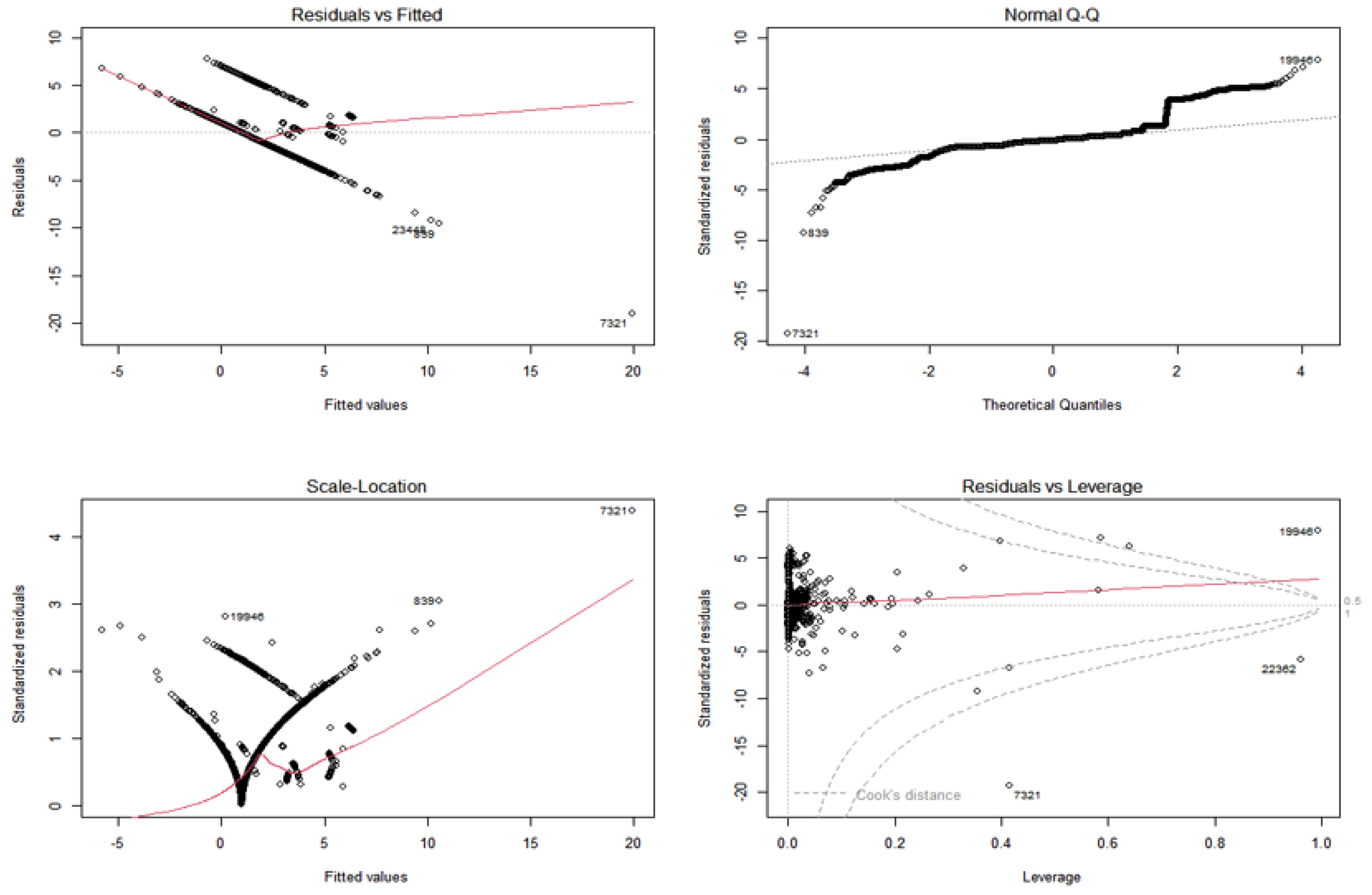
In our dataset, all features are numerical except one feature, date, which is removed, and the Linear Regression is constructed based on the full feature set. As depicted in Figure 1, the fitness of Linear Regression is under question since the normal distribution of Label as the dependent variable is not satisfied. Therefore, the suggested features for omission are not considered for omission. Also, Figure 1 shows some levels of multicollinearity among features, homoscedasticity, and the existence of outliers.

4.1.2. LASSO

Figure 2 shows the result of running LASSO on this dataset. According to this approach, 33 variables remain, and the rest should be omitted. We will use this reduced set later for the classification step.

4.1.3. Random Forest

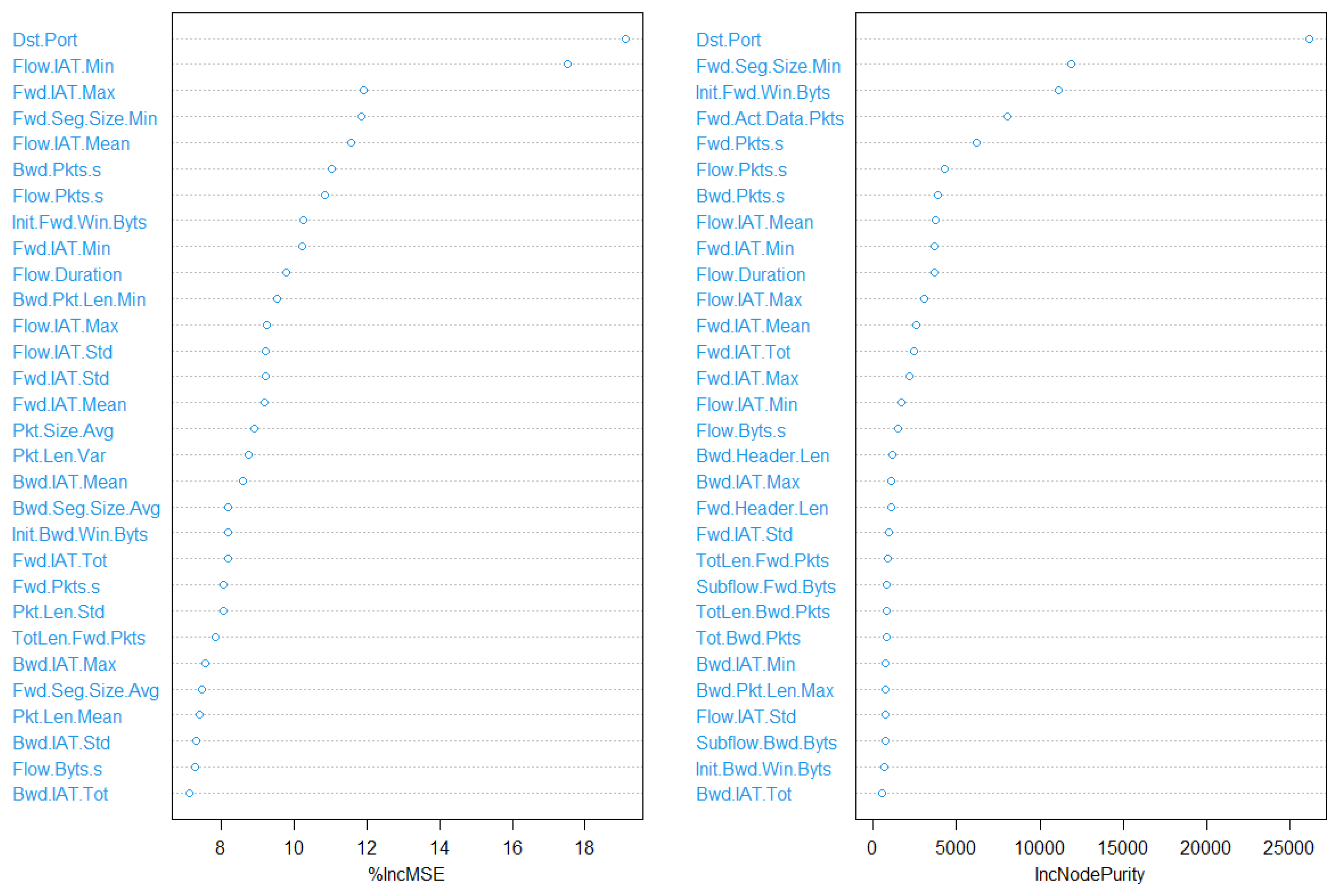
The Random Forest algorithm is implemented with 500 trees and 30 tries (variables). As illustrated in Figure 3, the resulting variable sets are not the same when calculated based on the two mentioned metrics. Thus, both results will be fed separately into the classifiers later.

4.1.4. Boruta

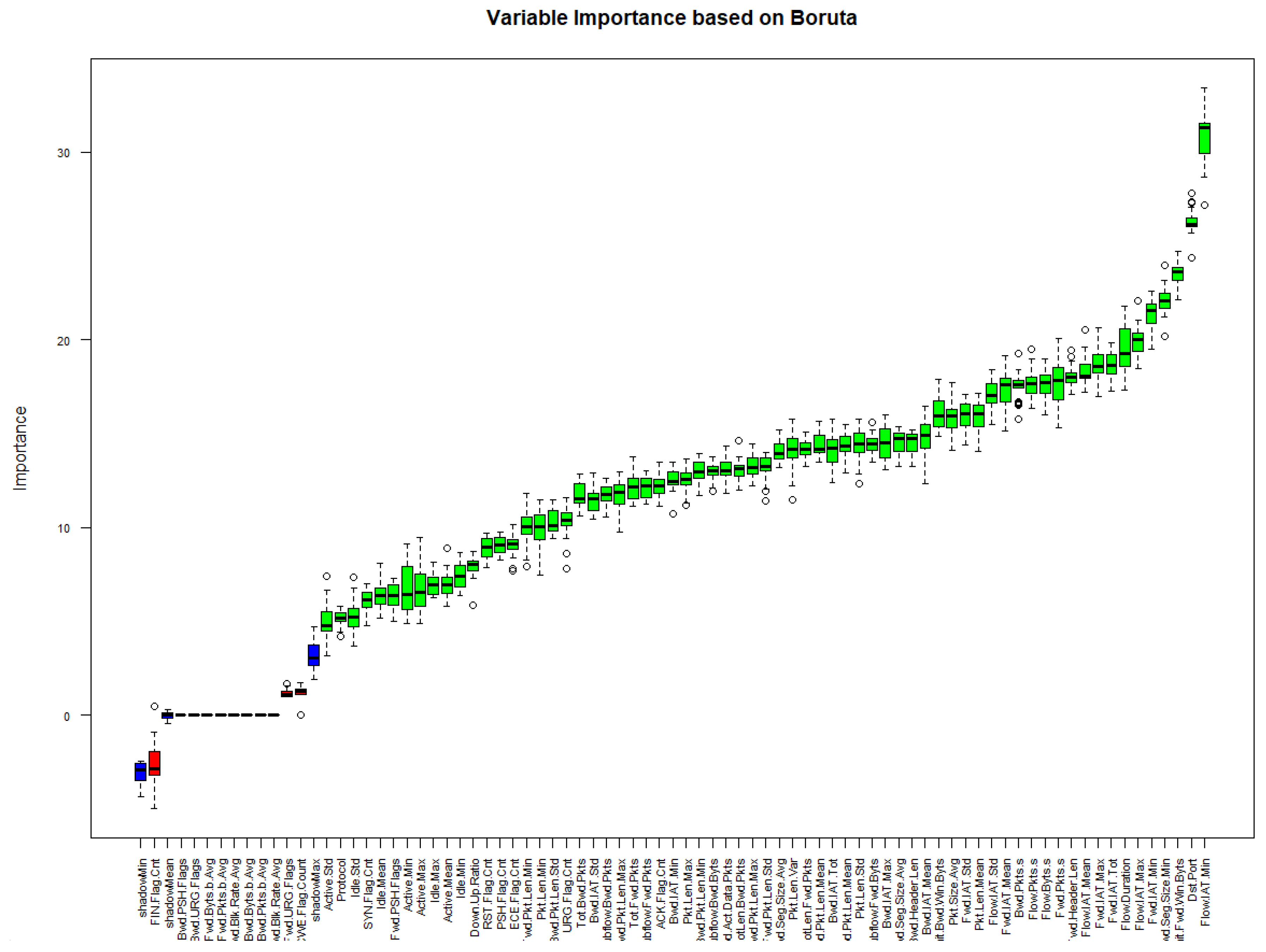
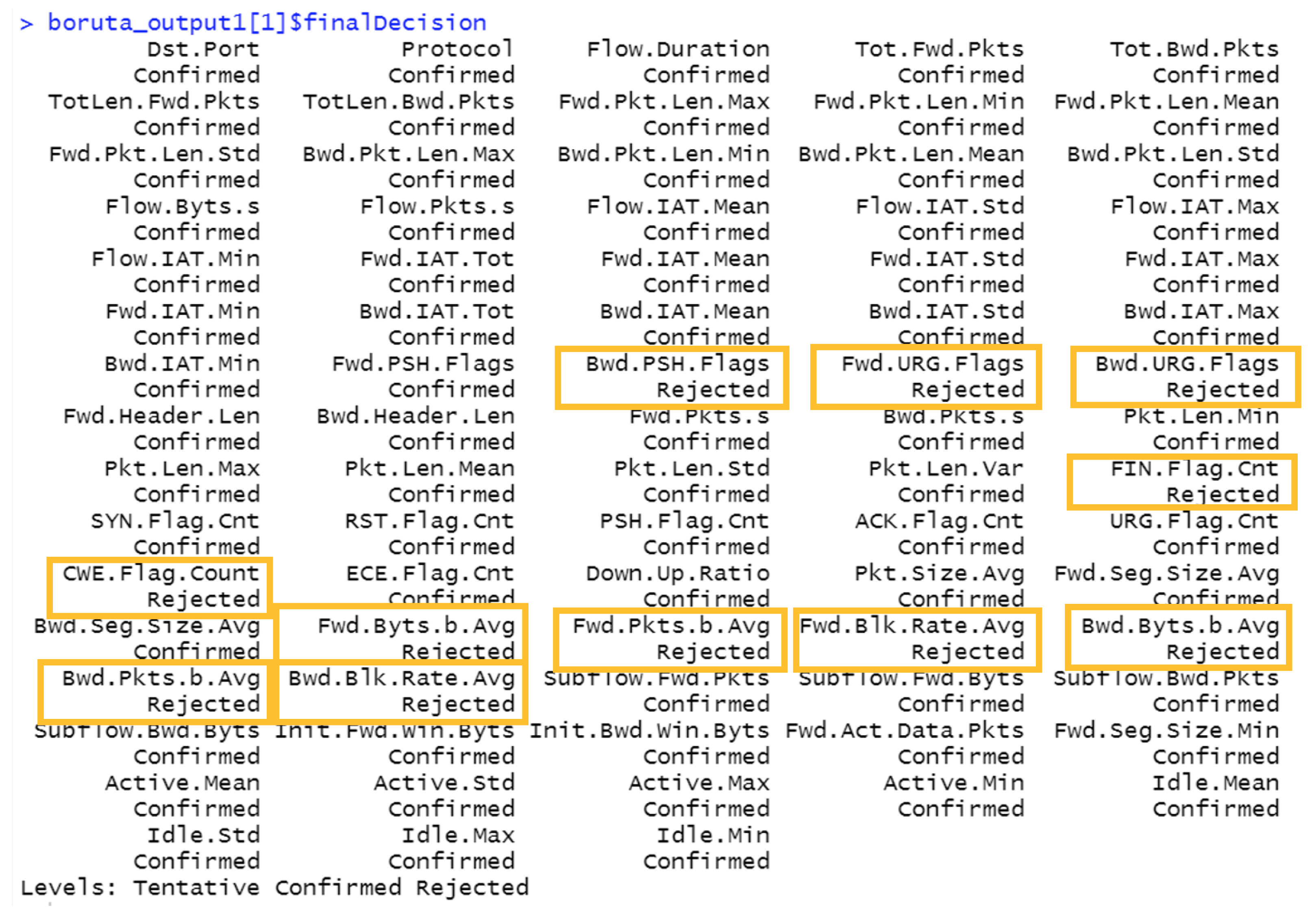
Figure 4 and Figure 5 illustrate the result of implementing the Boruta approach on the final train set. In Figure 4, the X axis shows each feature, and the Y axis depicts the value of each feature’s importance based on the Boruta technique. According to this technique, eleven features are suggested to be omitted (depicted as Rejected in Figure 5). The result of running different classifiers on the reduced set suggested by Boruta will be discussed later.

4.1.5. Autoencoders

We set the latent size or bottleneck to 30 and build six autoencoders. AE3 to AE6 follow the same structure as AE2, with different rates in their dropout layers. The loss function for this experiment is set to Categorical_Crossentropy, the optimizer to Adam, the number of epochs to 50, the batch size to 64, the activation function to Relu for all layers except the last layer, the activation function to Sigmoid for the last layer, and the layers include dense, dropout, and Leaky Relu activation layers. The configuration for each autoencoder and dropout rate is shown in

Table 4. Configuration for each autoencoder.

Autoencoder	Structure
AE1	5 Layers, No Dropout
AE2	10 Layers, No Dropout
AE3	AE2 Structure, Dropout rate = 0.25
AE4	AE2 Structure, Dropout rate = 0.1
AE5	AE2 Structure, Dropout rate = 0.5
AE6	AE2 Structure, Dropout rate = 0.75

. We set the dropout rate to 0.25, 0.1, 0.5, and 0.75 for AE3, AE4, AE5, and AE6, respectively.

4.2. Classifications

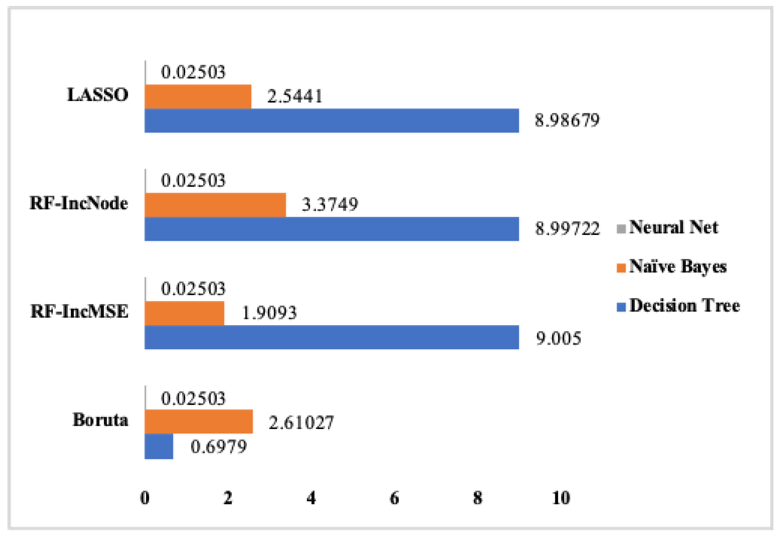
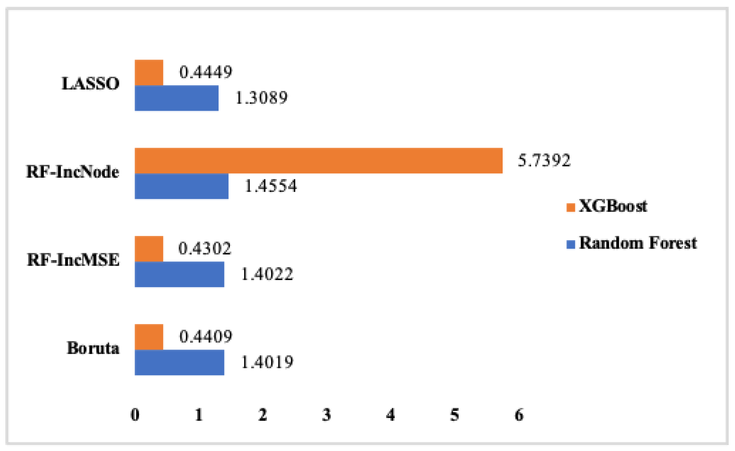
Figure 6, Figure 7, Figure 8 and Figure 9 summarize the difference between the RMSE values on running the classifiers on the train and test sets. As illustrated in Figure 9, the least difference of RMSE indicates the least amount of overfitting. The least RMSE value as the difference between running the classifiers on the train and the test sets is achieved from running Decision Tree on the reduced feature set captured from AE2, AE3, AE5, and AE6.

Also, we employed the KNN classifier on the first four reduced sets as depicted in

Table 5. Accuracy of KNN on the first four reduced sets.

K	Boruta	RF-IncMSE	RF-IncNode	K	LASSO
1	90.89	90.80	90.79	2	90.95
3	92.76	92.71	92.73	4	92.85
5	93.51	93.53	93.43	6	93.48
7	94.02	94.02	93.94	8	93.85
9	94.16	94.19	94.19	10	94.05
11	94.54	94.57	94.52	12	94.16
13	94.40	94.44	94.37	14	94.05
15	94.13	94.16	94.08	16	93.89
17	94.05	94.05	94.0	18	93.62
19	93.89	93.90	93.91	20	93.52

. The accuracy rate is very high for K equal to 11 for the first three reduced sets and K equal to 12 for the reduced set captured using the LASSO approach. The odd values of K for the first three sets are selected since the total number of samples was even numbered, but since LASSO deleted a few numbers of samples, and the total number of the remaining samples was odd for the last set, the even numbers of K are practised. However, since KNN is a lazy classifier, no signature-based model could be fetched. As a result, running other non-lazy classifiers could be a more promising solution.

5. Discussion

In this research, a subset of CSE-CIC-2018 dataset is used, and six feature reduction approaches have been investigated, including Linear Regression, Boruta, Random Forest with IncMSE, Random Forest with IncNodePurity, LASSO, and Autoencoders. The four sets captured from Boruta, LASSO, and two from Random Forest approaches were captured with the other six reduced sets fetched from autoencoders. Then, they were fed into three single-model classifiers as Decision Tree, Naïve Bayes, and neural networks, and two ensemble methods as Random Forest and XGBoost.

To determine the level of overfitting, we calculated the Root-Mean-Squared Error (RMSE) value between the train and test datasets for each model. We observed that the Decision Tree model demonstrated the lowest RMSE value when trained on the reduced feature set derived from autoencoders 2 (AE2), AE3, AE5, and AE6. This finding indicated that the structure of AE2 was particularly well-suited, showing comparable effectiveness to having dropout rates of 0.25%, 0.5%, and 0.75% on this architecture, respectively. Consequently, AE6 with a 75% dropout rate proved to be the least resource-intensive structure capable of producing signatures for all attack vectors while exhibiting the least amount of overfitting.

We evaluated our findings by implementing various classification approaches, such as XGBoost [16], Random Forest [17], and deep autoencoder as used in [15], among others. As depicted in Figure 6, Figure 7, Figure 8 and Figure 9, the Decision Tree model achieved the best results when applied to the reduced feature sets obtained from AE2, AE3, AE5, and AE6.

With regard to the efficiency of different approaches in our experiments, only Random Forest took a long time and the rest were somehow similar to each other. It is also worth mentioning that we removed the result of Principal Component Analysis (PCA) to change the feature space after implementing the autoencoders, as autoencoders already encompass PCA in a nonlinear fashion. Therefore, there is no need to have both PCA and autoencoders.

6. Conclusions and Future Work

In this research, we investigated feature and model overfitting reduction for network intrusion detection. We conducted our experiments on a subset of CSE-CIC-2018 dataset and analyzed feature reduction approaches, including Linear Regression, Boruta, Random Forest with IncMSE, Random Forest with IncNodePurity, LASSO, and autoencoders. We then fed the feature-reduced datasets into classifiers, including Decision Tree, Naïve Bayes, neural network, Random Forest, and XGBoost. Our experiments show that the Decision Tree classifier on autoencoders-based reduced sets of features yields the lowest overfitting among all the combinations.

For future work, we plan to leverage deep learning-based classifiers such as LSTM (Long Short-Term Memory) or convolutional neural networks (CNNs) to further enhance detection performance. Additionally, we aim to refine the autoencoder’s structure for feature construction, aiming to achieve a higher detection rate while minimizing overfitting. Furthermore, we aspire to evaluate the impact of our proposed approaches on the detection rate of different classes of attack vectors separately. By understanding the strengths and weaknesses of our techniques on specific attack types, we can tailor our solution to be more robust and effective across various threat scenarios. Another aspect of our future research involves adapting our solution to handle class imbalance effectively. Real-world datasets exhibit imbalanced class distributions, where certain attack types might be significantly under-represented compared to others. Devising methods to handle class imbalance will be pivotal in ensuring the reliability and fairness of our model in practical deployment scenarios.

References

- NIST SP 800-53 Rev. 5; Security and Privacy Controls for Information Systems and Organizations. National Institute of Standards and Technology: Gaithersburg, MD, USA, 2020. [CrossRef]
- Khan, R.U.; Zhang, X.; Alazab, M.; Kumar, R. An Improved Convolutional Neural Network Model for Intrusion Detection in Networks. In Proceedings of the 2019 Cybersecurity and Cyberforensics Conference (CCC), Melbourne, Australia, 8–9 May 2019; pp. 74–77. [Google Scholar] [CrossRef]
- Shapoorifard, H.; Shamsinejad, P. Intrusion Detection using a Novel Hybrid Method Incorporating an Improved KNN. Int. J. Comput. Appl. 2017, 173, 5–9. [Google Scholar] [CrossRef]
- Chkirbene, Z.; Erbad, A.; Hamila, R.; Mohamed, A.; Guizani, M.; Hamdi, M. TIDCS: A Dynamic Intrusion Detection and Classification System Based Feature Selection. IEEE Access 2020, 8, 95864–95877. [Google Scholar] [CrossRef]
- Leevy, J.L.; Khoshgoftaar, T.M. A survey and analysis of intrusion detection models based on CSE-CIC-IDS2018 Big Data. J. Big Data 2020, 7, 104. [Google Scholar] [CrossRef]
- Li, X.; Chen, W.; Zhang, Q.; Wu, L. Building Auto-Encoder Intrusion Detection System based on random forest feature selection. Comput. Secur. 2020, 95, 101851. [Google Scholar] [CrossRef]
- Laghrissi, F.; Douzi, S.; Douzi, K.; Hssina, B. Intrusion detection systems using long short-term memory (LSTM). J. Big Data 2021, 8, 65. [Google Scholar] [CrossRef]
- KDD’99 Dataset. Available online: http://kdd.ics.uci.edu/databases/kddcup99/kddcup99.html (accessed on 6 July 2023).
- NSL-KDD Dataset. Available online: https://www.unb.ca/cic/datasets/nsl.html (accessed on 6 July 2023).
- Intrusion Detection Evaluation Dataset (CIC-IDS2017). Available online: https://www.unb.ca/cic/datasets/ids-2017.html (accessed on 6 July 2023).
- CSE-CIC-IDS2018 on AWS. Available online: https://www.unb.ca/cic/datasets/ids-2018.html (accessed on 6 July 2023).
- Shen, Y.; Zheng, K.; Wu, C.; Zhang, M.; Niu, X.; Yang, Y. An ensemble method based on selection using bat algorithm for intrusion detection. Comput. J. 2018, 61, 526–538. [Google Scholar] [CrossRef]
- Mirsky, Y.; Doitshman, T.; Elovici, Y.; Shabtai, A. Kitsune: An Ensemble of Autoencoders for Online Network Intrusion Detection. In Proceedings of the 2018 Network and Distributed System Security Symposium (NDSS), Internet Society, San Diego, CA, USA, 18–21 February 2018. [Google Scholar] [CrossRef]
- Basnet, R.B.; Shash, R.; Johnson, C.; Walgren, L.; Doleck, T. Towards Detecting and Classifying Network Intrusion Traffic Using Deep Learning Frameworks. J. Internet Serv. Inf. Secur. 2019, 9, 1–17. [Google Scholar]
- Catillo, M.; Rak, M.; Villano, U. 2L-ZED-IDS: A Two-Level Anomaly Detector for Multiple Attack Classes. In Proceedings of the Web, Artificial Intelligence and Network Applications; Barolli, L., Amato, F., Moscato, F., Enokido, T., Takizawa, M., Eds.; Springer: Cham, Switzerland, 2020; pp. 687–696. [Google Scholar]
- D’hooge, L.; Wauters, T.; Volckaert, B.; De Turck, F. Inter-dataset generalization strength of supervised machine learning methods for intrusion detection. J. Inf. Secur. Appl. 2020, 54, 102564. [Google Scholar] [CrossRef]
- Lima Filho, F.S.d.; Silveira, F.A.; de Medeiros Brito Junior, A.; Vargas-Solar, G.; Silveira, L.F. Smart detection: An online approach for DoS/DDoS attack detection using machine learning. Secur. Commun. Netw. 2019, 2019, 1574749. [Google Scholar] [CrossRef]
- Karatas, G.; Demir, O.; Sahingoz, O.K. Increasing the Performance of Machine Learning-Based IDSs on an Imbalanced and Up-to-Date Dataset. IEEE Access 2020, 8, 32150–32162. [Google Scholar] [CrossRef]
- Kim, J.; Kim, J.; Kim, H.; Shim, M.; Choi, E. CNN-Based Network Intrusion Detection against Denial-of-Service Attacks. Electronics 2020, 9, 916. [Google Scholar] [CrossRef]
- IDS 2018 Intrusion CSVs (CSE-CIC-IDS2018). Available online: https://www.kaggle.com/datasets/solarmainframe/ids-intrusion-csv (accessed on 6 July 2023).
- Tibshirani, R. Regression shrinkage and selection via the lasso. J. R. Stat. Soc. Ser. B Stat. Methodol. 1996, 58, 267–288. [Google Scholar]
- Breiman, L. Random forests. Mach. Learn. 2001, 45, 5–32. [Google Scholar] [CrossRef]
- Kursa, M.B.; Rudnicki, W.R. Feature Selection with the Boruta Package. J. Stat. Softw. 2010, 36, 1–13. [Google Scholar] [CrossRef]
- Rumelhart, D.E.; McClelland, J.L. Learning Internal Representations by Error Propagation. In Parallel Distributed Processing: Explorations in the Microstructure of Cognition: Foundations; MIT Press: Cambridge, MA, USA, 1987; pp. 318–362. [Google Scholar]