Figure 1.
Connected nodes in an MioT environment.
Figure 1.
Connected nodes in an MioT environment.
Figure 2.
Connected nodes in a CioT environment.
Figure 2.
Connected nodes in a CioT environment.
Figure 3.
An example of an IoT bot attack against a CioT system to launch a large-scale DDoS attack.
Figure 3.
An example of an IoT bot attack against a CioT system to launch a large-scale DDoS attack.
Figure 4.
A block diagram of an autoencoder model.
Figure 4.
A block diagram of an autoencoder model.
Figure 5.
The research methodology conceptual model.
Figure 5.
The research methodology conceptual model.
Figure 6.
PiB dataset with normal and anomalous class distributions.
Figure 6.
PiB dataset with normal and anomalous class distributions.
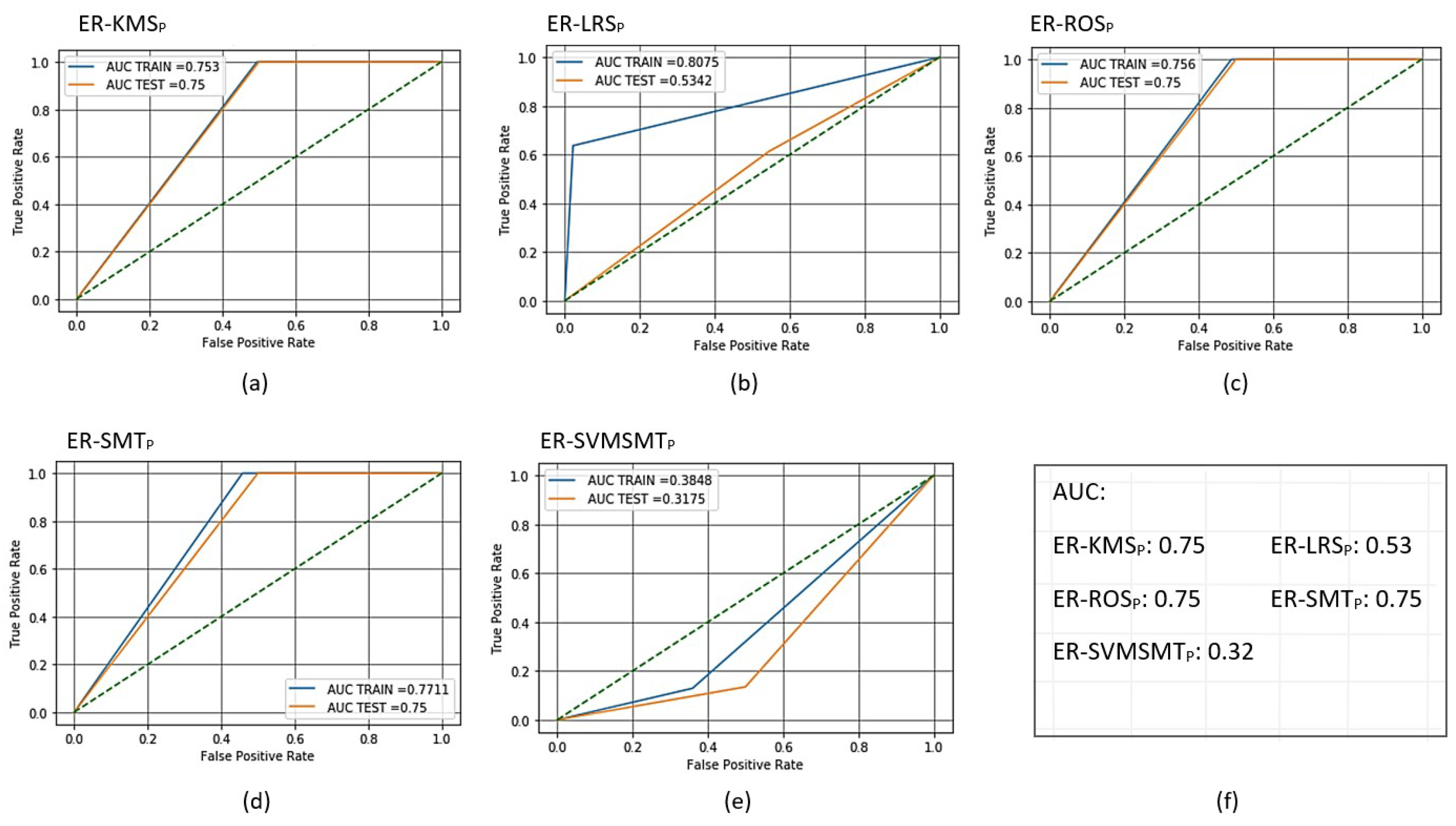
Figure 7.
Receiver operating characteristic (ROC) curves for the trained and scored PCA-based AMiDS using oversampling methods based on the five experimental runs, respectively: (a) ER-KMS, (b) ER-LRS, (c) ER-ROS, (d) ER-SMT, and (e) ER-SVMSMT. Summary of the AUC values based on the experimental runs according to the applied methods is shown in (f).
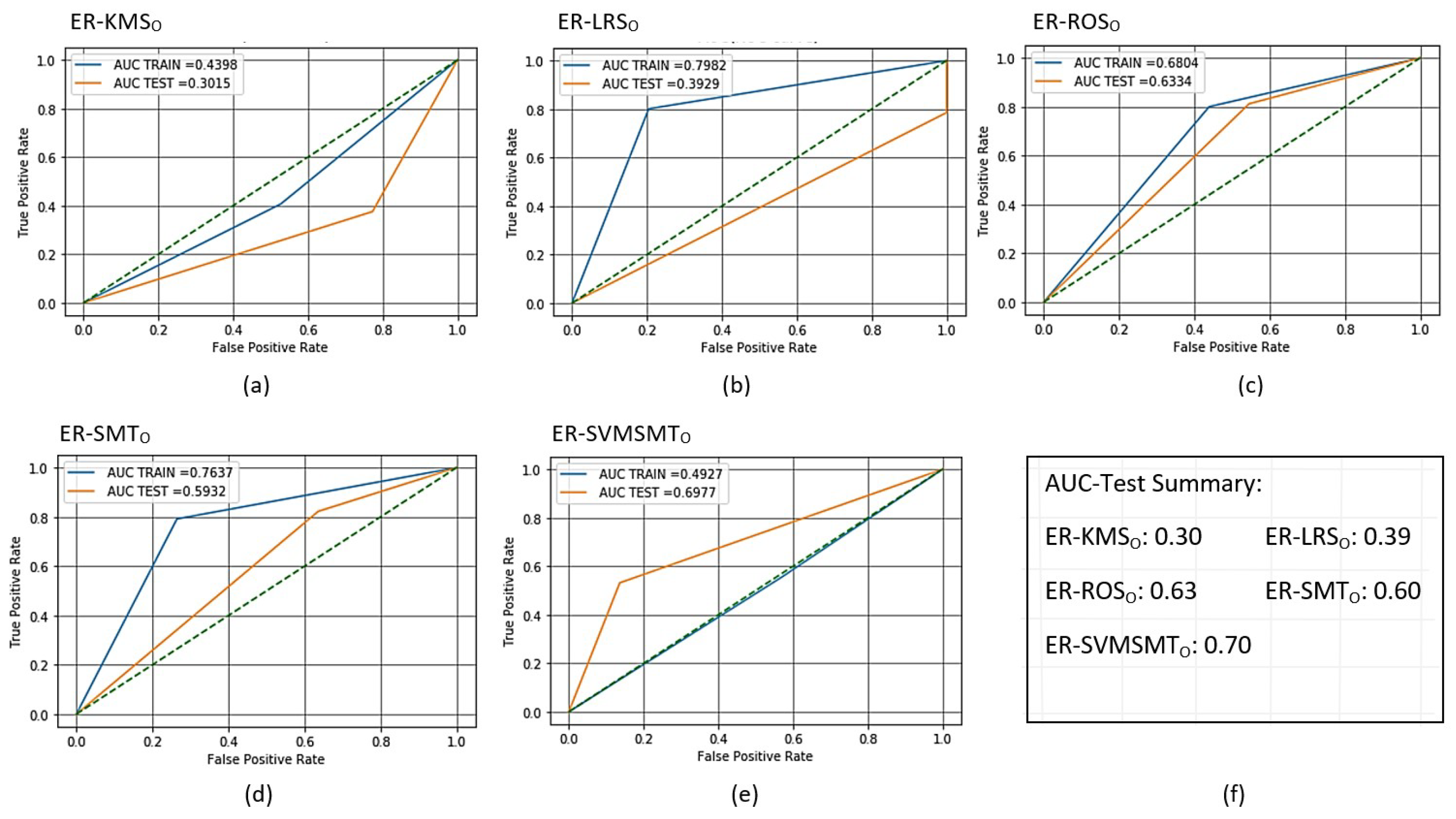
Figure 8.
Receiver operating characteristic (ROC) curves for the trained and scored oSVM-based AMiDS using oversampling methods based on the five experimental runs, respectively: (a) ER-KMS, (b) ER-LRS, (c) ER-ROS, (d) ER-SMT, and (e) ER-SVMSMT. Summary of the AUC values based on the experimental runs according to the applied methods is shown in (f).
Figure 9.
Receiver operating characteristic (ROC) curves for the trained and scored PCA- and oSVM-based AMiDS using hybrid methods based on the four experimental runs, respectively: (a) ER-SMTEN for PCA, (b) ER-SMTEK for PCA, (d) ER-SMTEN for oSVM, and (e) ER-SMTEK for oSVM. Summary of the AUC values based on the experimental runs according to the applied methods is shown in (c) and (f) for the PCA- and oSVM-based AMiDS, respectively.
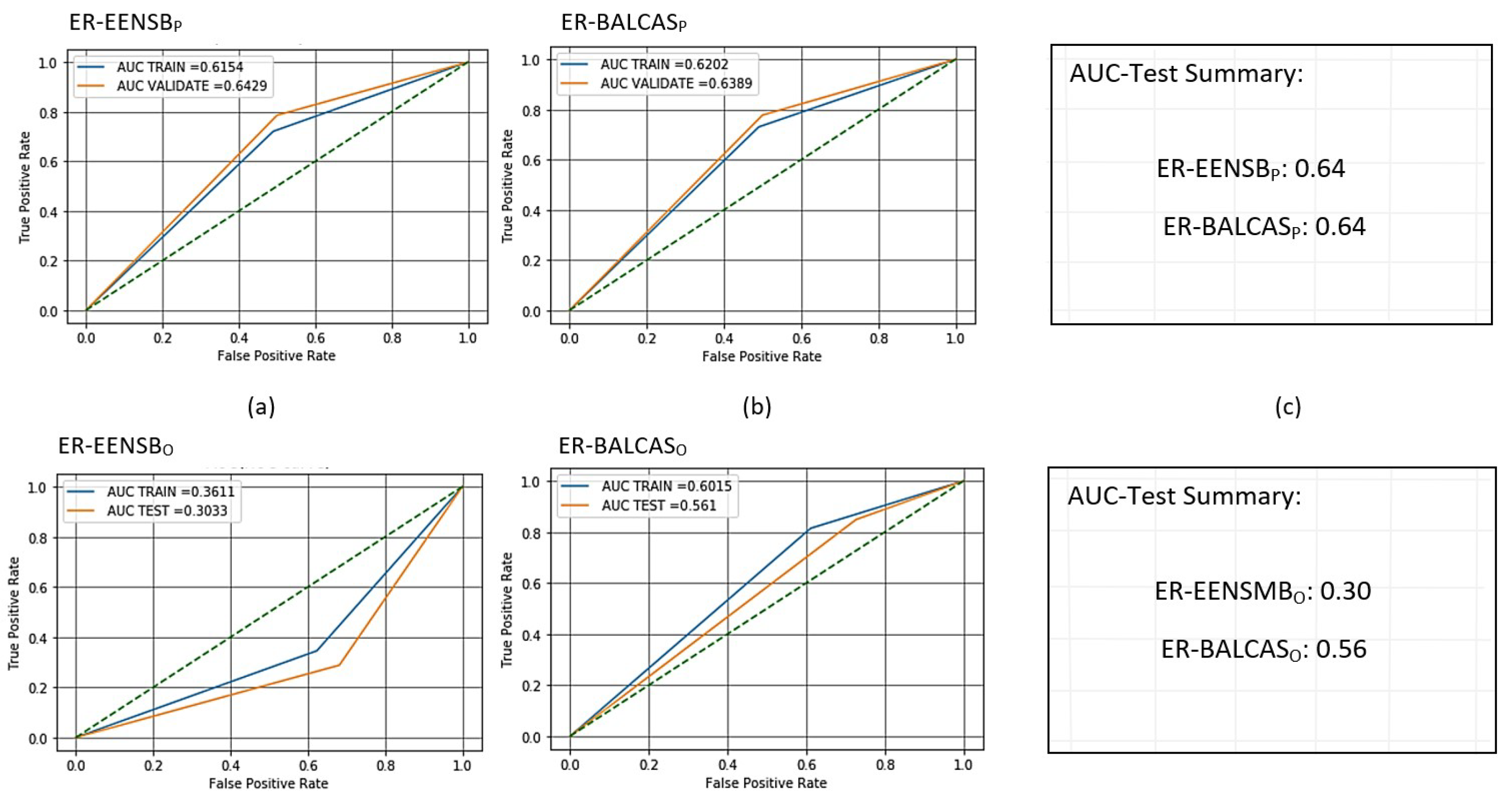
Figure 10.
Receiver operating characteristic (ROC) curves for trained and scored PCA- and oSVM-based AMiDS using ensemble-based methods based on the four experimental runs, respectively: (a) ER-EENSB for PCA, (b) ER-BALCAS for PCA, (d) ER-EENSB for oSVM, and (e) ER-BALCAS for oSVM. Summary of the AUC values based on the experimental runs according to the applied methods is shown in (c) and (f) for the PCA- and oSVM-based AMiDS, respectively.
Figure 11.
The Autoencoder (AE) model history and parameters for the PCA- and OSVM-based AMiDS models.
Figure 11.
The Autoencoder (AE) model history and parameters for the PCA- and OSVM-based AMiDS models.
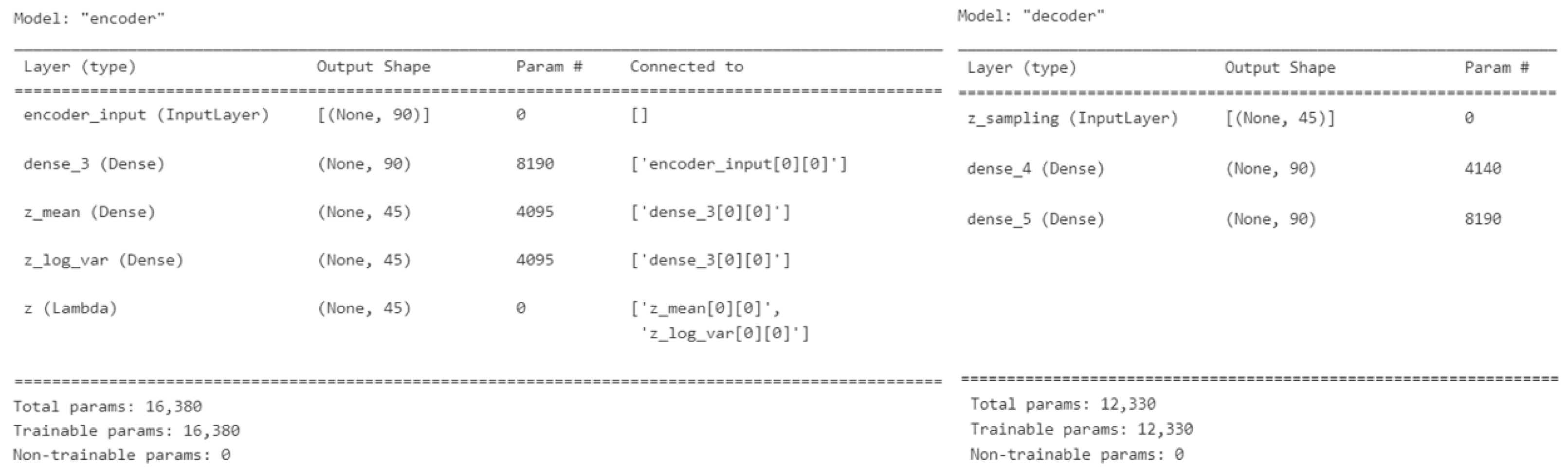
Figure 12.
Variational Autoencoder Oversampler (VAEOversampler) encoder and decoder parameters for the PCA- and OSVM-based AMiDS models.
Figure 12.
Variational Autoencoder Oversampler (VAEOversampler) encoder and decoder parameters for the PCA- and OSVM-based AMiDS models.
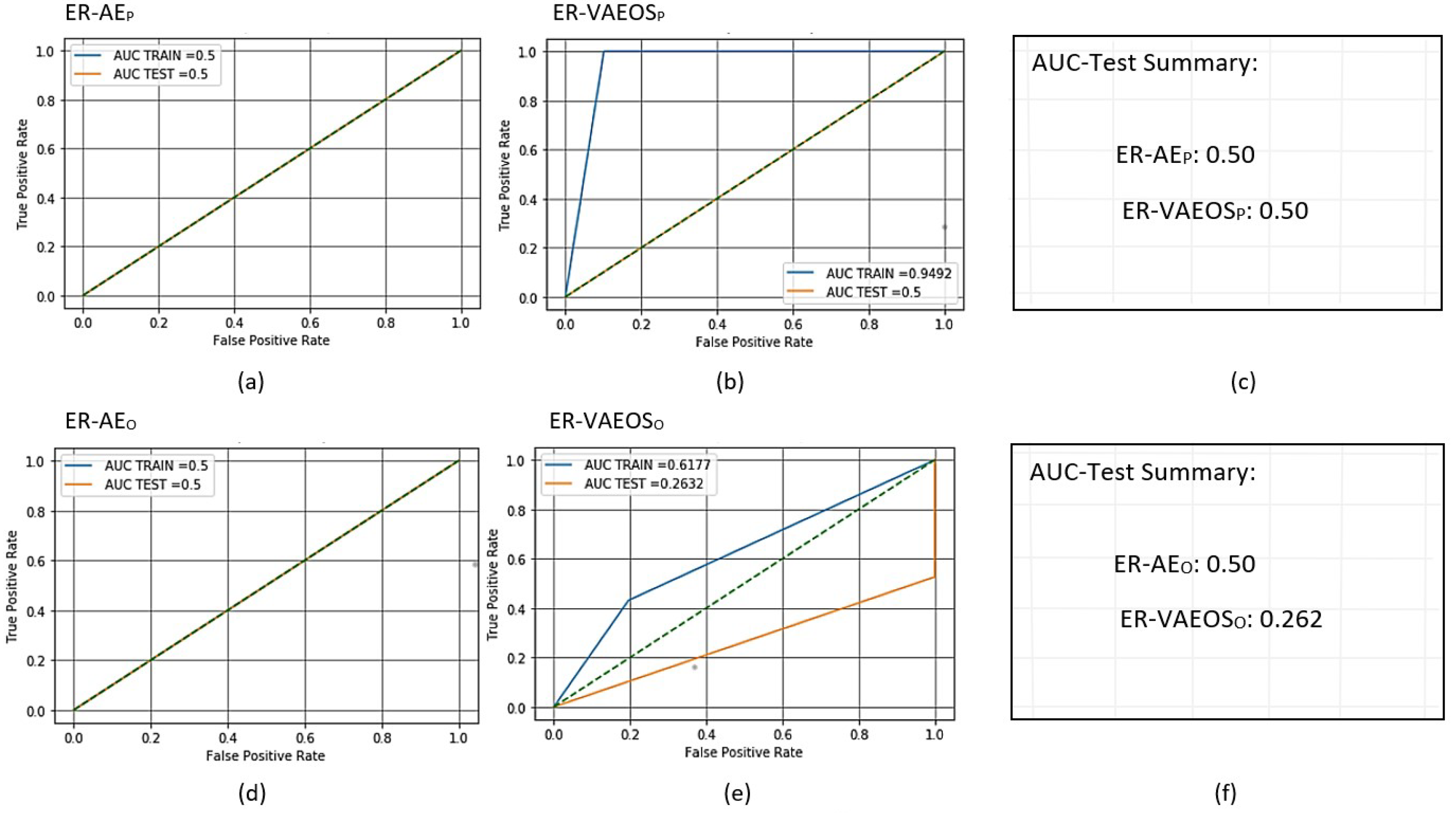
Figure 13.
Receiver operating characteristic (ROC) curves for trained and scored PCA- and oSVM-based AMiDS using generative-based methods based on the four experimental runs, respectively: (a) ER-AE for PCA, (b) ER-VAEO for PCA, (d) ER-AE for oSVM, and (e) ER-VAEO for oSVM. Summary of the AUC values based on the experimental runs according to the applied methods is shown in (c) and (f) for the PCA- and oSVM-based AMiDS, respectively.
Figure 14.
tSVM AMiDS baseline model performance.
Figure 14.
tSVM AMiDS baseline model performance.
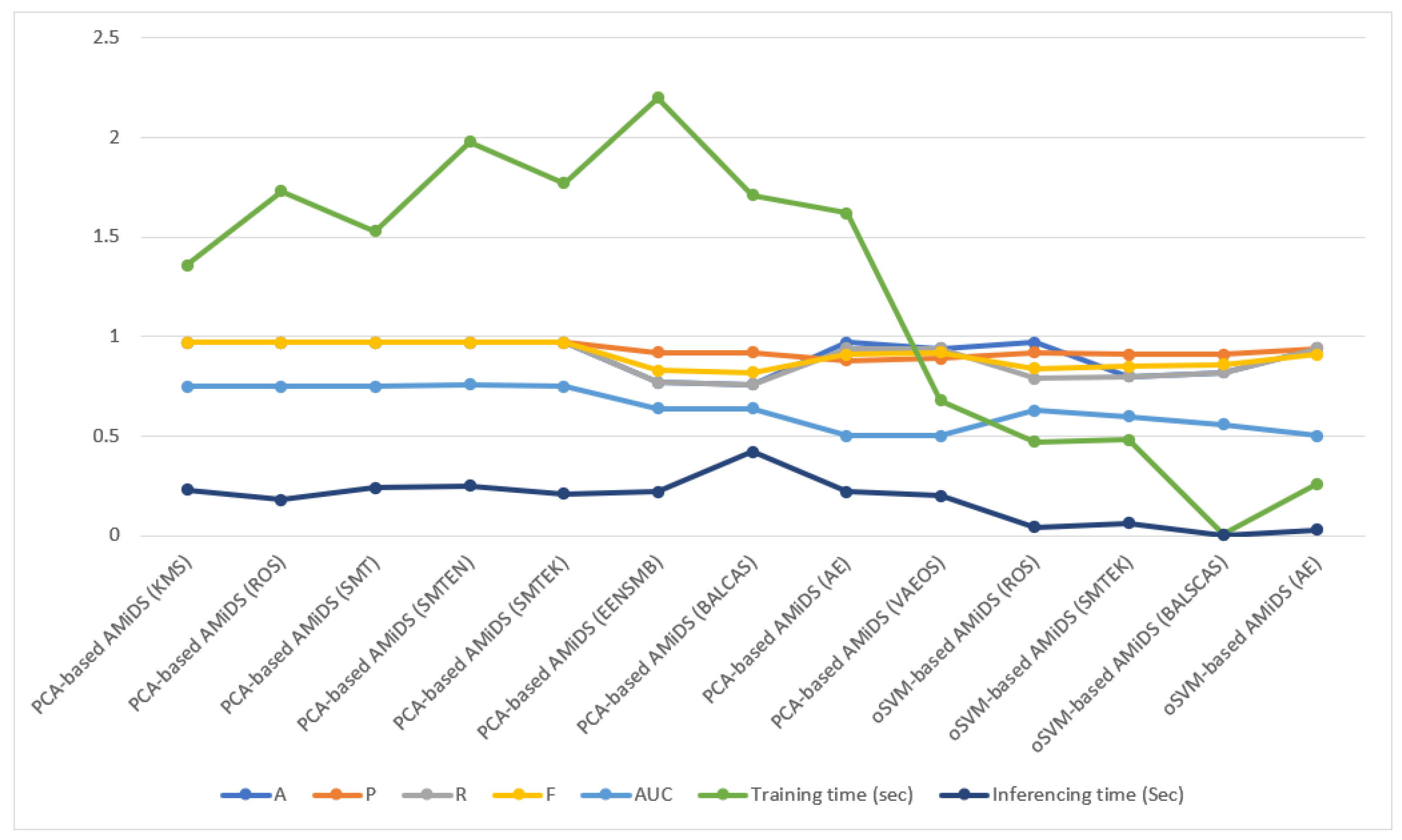
Figure 15.
Better-case scored AMiDS model performance based on the weighted average.
Figure 15.
Better-case scored AMiDS model performance based on the weighted average.
Table 1.
Description of data-level methods for imbalanced learning.
Table 1.
Description of data-level methods for imbalanced learning.
| Method | Description | References |
|---|
| Autoencoder (AE) | A deep learning method used to generate synthetic data using unsupervised learning. It consists of an encoder and a decoder. The encoder compresses the input data into a non-regularized latent space, and the decoder learns the latent space distribution to reconstruct the data such that they are closer to the original but not exactly the same. However, in our implementation, we use L1 regularization to enable the autoencoder to learn any important features in the latent space and to avoid overfitting. | [49] |
| BalanceCascade | Similar to EasyEnsemble, except it undersamples the majority class by deleting examples using supervised deletion rather than random deletion. | [50,51] |
| EasyEnsemble | Uses an undersampling approach efficiently to randomly generate several subsets from the majority class examples without ignoring useful information. It then combines each generated subset with the minority class samples, where the size of the subset is similar to the size of the minority class examples to train an adaboost ensemble. | [50,51] |
| KMeanSMOTE | Combines k-means clustering and SMOTE oversampling to balance the data while avoiding unnecessary noise generation. | [52] |
| LoRAS | Generates Gaussian noise in small neighborhoods around the minority class examples and uses multiple noisy data points to create the synthesized data. | [53] |
| Random Oversampler (ROS) | Selects random examples from the minority class and then uses replacement to add the selected examples to the dataset, thus providing duplicate instances from the minority class in the dataset. | [2,54] |
| SMOTE | Resamples the minority class by creating synthetic examples instead of replacing them. | [55] |
| SMOTEEN | Applies oversampling using SMOTE followed by undersampling using the Edited Nearest Neighbor (ENN*) to provide in-depth data cleaning. It removes examples from both the minority and majority classes, performing better when the dataset contains a small number of positive examples. | [56] |
| SMOTETomek | Applies oversampling using SMOTE followed by Tomek links to clean the data by removing fewer examples from both the minority and majority classes compared to the SMOTEEN method. However, similar to SMOTEEN, it performs better on datasets with a small number of positive examples. | [56] |
| SVMSMOTE | Applies SVM to find the borderline area and SMOTE oversampling to randomly generate artificial data along the obtained borderline, thus establishing a clear boundary between the majority and minority classes. | [2] |
| Variational Autoencoder (VAE) | Structurally similar to an AE, except that the input, latent representation, and output are probabilistic random variables. In addition, the encoder compresses the data into a regularized latent space, while the decoder takes the latent representation as an input and outputs a probability distribution of the data. | [57] |
Table 2.
Classification of data-level methods for imbalanced learning.
Table 2.
Classification of data-level methods for imbalanced learning.
| Method | Oversampling | Hybrid | Generative | Ensemble | References |
|---|
| Autoencoder (AE) | ✗ | ✗ | ✓ | ✗ | [46,58] |
| BalanceCascade | ✗ | ✗ | ✗ | ✓ | [50,51,59,60] |
| EasyEnsemble | ✗ | ✗ | ✗ | ✓ | [50,51,60] |
| KMeanSMOTE | ✓ | ✗ | ✗ | ✗ | [52,61] |
| LoRAS | ✓ | ✗ | ✗ | ✗ | [53,62] |
| Random Oversampler (ROS) | ✓ | ✗ | ✗ | ✗ | [2,54,61] |
| SMOTE | ✓ | ✗ | ✗ | ✗ | [2,55,61,63,64,65] |
| SMOTEEN | ✗ | ✓ | ✗ | ✗ | [2,56,61,65] |
| SMOTETomek | ✗ | ✓ | ✗ | ✗ | [2,56,61,65,66,67] |
| SVMSMOTE | ✓ | ✗ | ✗ | ✗ | [2,61,65] |
| Variational Autoencoder (VAE) | ✗ | ✗ | ✓ | ✗ | [34,35,68] |
Table 3.
Features of the PiB dataset.
Table 3.
Features of the PiB dataset.
| ID | Feature | Type | Description |
|---|
| 1 | pkSeqID | Number | Row Identifier |
| 2 | Stime | Time | Record start time |
| 3 | flgs | String | Flow state flags seen in transactions |
| 4 | proto | String | Textual representation of transaction protocols present in network flow |
| 5 | saddr | IP address | Source IP address |
| 6 | sport | Number | Source port number |
| 7 | daddr | IP address | Destination IP address |
| 8 | dport | Number | Destination port number |
| 9 | pkts | Number | Total count of packets in transaction |
| 10 | bytes | Number | Total number of bytes in transaction |
| 11 | state | String | Transaction state |
| 12 | ltime | Time | Record last time |
| 13 | seq | Number | Argus sequence number |
| 14 | dur | Number | Record total duration |
| 15 | mean | Number | Average duration of aggregated records |
| 16 | stddev | Number | Standard deviation of aggregated records |
| 17 | sum | Number | Total duration of aggregated records |
| 18 | min | Number | Minimum duration of aggregated records |
| 19 | max | Number | Maximum duration of aggregated records |
| 20 | spkts | Number | Source-to-destination packet count |
| 21 | dpkts | Number | Destination-to-source packet count |
| 22 | sbytes | Number | Source-to-destination byte count |
| 23 | dbytes | Number | Destination-to-source byte count |
| 24 | rate | Number | Total packets per second in transaction |
| 25 | srate | Number | Source-to-destination packets per second |
| 26 | drate | Number | Destination-to-source packets per second |
| 27 | label | Number | Class label: 0 for Normal traffic, 1 for Attack Traffic |
| 28 | category | String | Traffic category |
| 29 | subcategory | String | Traffic subcategory |
Table 4.
Trained PCA-based AMiDS evaluation results for the oversampling methods based on the weighted average.
Table 4.
Trained PCA-based AMiDS evaluation results for the oversampling methods based on the weighted average.
| Method | A | P | R | F | AUC | Training Time (s) | Inference Time (s) | No. of Examples |
|---|
| ER-KMS | 0.75 | 0.83 | 0.75 | 0.74 | 0.753 | 1.362 | ... | 2992 |
| ER-LRS | 0.81 | 0.85 | 0.81 | 0.80 | 0.875 | 1.6996 | ... | 2992 |
| ER-ROS | 0.76 | 0.84 | 0.76 | 0.74 | 0.756 | 1.7299 | ... | 2992 |
| ER-SMT | 0.77 | 0.84 | 0.77 | 0.76 | 0.771 | 1.5325 | ... | 2992 |
| ER-SVMSMT | 0.29 | 0.39 | 0.29 | 0.25 | 0.385 | 1.5394 | ... | 2161 |
Table 5.
Trained PCA-based AMiDS evaluation results for the oversampling methods based on the normal case.
Table 5.
Trained PCA-based AMiDS evaluation results for the oversampling methods based on the normal case.
| Method | A | P | R | F | AUC | Training Time (s) | Inference Time (s) | No. of Examples |
|---|
| ER-KMS | ... | 1.00 | 0.51 | 0.67 | ... | ... | ... | 1496 |
| ER-LRS | ... | 0.73 | 0.98 | 0.84 | ... | ... | ... | 1496 |
| ER-ROS | ... | 1.00 | 0.51 | 0.68 | ... | ... | ... | 1469 |
| ER-SMT | ... | 1.00 | 0.54 | 0.70 | ... | ... | ... | 1496 |
| ER-SVMSMT | ... | 0.25 | 0.64 | 0.36 | ... | ... | ... | 655 |
Table 6.
Trained PCA-based AMiDS evaluation results for the oversampling methods based on the anomalous case.
Table 6.
Trained PCA-based AMiDS evaluation results for the oversampling methods based on the anomalous case.
| Method | A | P | R | F | AUC | Training Time (s) | Inference Time (s) | No. of Examples |
|---|
| ER-KMS | ... | 0.67 | 1.0 | 0.80 | ... | ... | ... | 1496 |
| ER-LRS | ... | 0.97 | 0.64 | 0.77 | ... | ... | ... | 1496 |
| ER-ROS | ... | 0.67 | 1.00 | 0.80 | ... | ... | ... | 1496 |
| ER-SMT | ... | 0.69 | 1.00 | 0.81 | ... | ... | ... | 1496 |
| ER-SVMSMT | ... | 0.45 | 0.13 | 0.20 | ... | ... | ... | 1496 |
Table 7.
Scored PCA-based AMiDS evaluation results for the oversampling methods based on the weighted average.
Table 7.
Scored PCA-based AMiDS evaluation results for the oversampling methods based on the weighted average.
| Method | A | P | R | F | AUC | Training Time (s) | Inference Time (s) | No. of Examples |
|---|
| ER-KMS | 0.97 | 0.97 | 0.97 | 0.97 | 0.75 | ... | 0.2249 | 400 |
| ER-LRS | 0.60 | 0.90 | 0.60 | 0.71 | 0.534 | ... | 0.2090 | 400 |
| ER-ROS | 0.97 | 0.97 | 0.97 | 0.97 | 0.75 | ... | 0.1820 | 400 |
| ER-SMT | 0.97 | 0.97 | 0.97 | 0.97 | 0.75 | ... | 0.2347 | 400 |
| ER-SVMSMT | 0.15 | 0.78 | 0.15 | 0.22 | 0.318 | ... | 0.2133 | 400 |
Table 8.
Scored PCA-based AMiDS evaluation results for the oversampling methods based on the normal case.
Table 8.
Scored PCA-based AMiDS evaluation results for the oversampling methods based on the normal case.
| Method | A | P | R | F | AUC | Training Time (s) | Inference Time (s) | No. of Examples |
|---|
| ER-KMS | ... | 1.00 | 0.50 | 0.67 | ... | ... | ... | 22 |
| ER-LRS | ... | 0.06 | 0.45 | 0.11 | ... | ... | ... | 22 |
| ER-ROS | ... | 1.00 | 0.50 | 0.67 | ... | ... | ... | 22 |
| ER-SMT | ... | 1.00 | 0.50 | 0.67 | ... | ... | ... | 22 |
| ER-SVMSMT | ... | 0.03 | 0.50 | 0.06 | ... | ... | ... | 22 |
Table 9.
Scored PCA-based AMiDS evaluation results for the oversampling methods based on the anomalous case.
Table 9.
Scored PCA-based AMiDS evaluation results for the oversampling methods based on the anomalous case.
| Method | A | P | R | F | AUC | Training Time (s) | Inference Time (s) | No. of Examples |
|---|
| ER-KMS | ... | 0.97 | 1.0 | 0.99 | ... | ... | ... | 378 |
| ER-LRS | ... | 0.95 | 0.61 | 0.75 | ... | ... | ... | 378 |
| ER-ROS | ... | 0.97 | 1.00 | 0.99 | ... | ... | ... | 378 |
| ER-SMT | ... | 0.97 | 1.00 | 0.99 | ... | ... | ... | 378 |
| ER-SVMSMT | ... | 0.82 | 0.13 | 0.23 | ... | ... | ... | 378 |
Table 10.
Trained oSVM-based AMiDS evaluation results for the oversampling methods based on the weighted average.
Table 10.
Trained oSVM-based AMiDS evaluation results for the oversampling methods based on the weighted average.
| Method | A | P | R | F | AUC | Training Time (s) | Inference Time (s) | No. of Examples |
|---|
| ER-KMS | 0.44 | 0.44 | 0.44 | 0.44 | 0.440 | 0.676 | ... | 2393 |
| ER-LRS | 0.80 | 0.80 | 0.80 | 0.80 | 0.789 | 0.727 | ... | 2393 |
| ER-ROS | 0.68 | 0.69 | 0.68 | 0.67 | 0.680 | 0.466 | ... | 2393 |
| ER-SMT | 0.76 | 0.76 | 0.76 | 0.76 | 0.764 | 0.456 | ... | 2393 |
| ER-SVMSMT | 0.52 | 0.57 | 0.52 | 0.53 | 0.493 | 0.256 | ... | 1728 |
Table 11.
Trained oSVM-based AMiDS evaluation results for the oversampling methods based on the normal case.
Table 11.
Trained oSVM-based AMiDS evaluation results for the oversampling methods based on the normal case.
| Method | A | P | R | F | AUC | Training Time (s) | Inference Time (s) | No. of Examples |
|---|
| ER-KMS | ... | 0.45 | 0.47 | 0.46 | ... | ... | ... | 1206 |
| ER-LRS | ... | 0.80 | 0.80 | 0.80 | ... | ... | ... | 1206 |
| ER-ROS | ... | 0.74 | 0.56 | 0.64 | ... | ... | ... | 1206 |
| ER-SMT | ... | 0.78 | 0.74 | 0.76 | ... | ... | ... | 1206 |
| ER-SVMSMT | ... | 0.30 | 0.43 | 0.35 | ... | ... | ... | 529 |
Table 12.
Trained oSVM-based AMiDS evaluation results for the oversampling methods based on the anomalous case.
Table 12.
Trained oSVM-based AMiDS evaluation results for the oversampling methods based on the anomalous case.
| Method | A | P | R | F | AUC | Training Time (s) | Inference Time (s) | No. of Examples |
|---|
| ER-KMS | ... | 0.43 | 0.41 | 0.42 | ... | ... | ... | 1187 |
| ER-LRS | ... | 0.79 | 0.80 | 0.80 | ... | ... | ... | 1187 |
| ER-ROS | ... | 0.64 | 0.80 | 0.71 | ... | ... | ... | 1187 |
| ER-SMT | ... | 0.75 | 0.79 | 0.77 | ... | ... | ... | 1187 |
| ER-SVMSMT | ... | 0.69 | 0.56 | 0.62 | ... | ... | ... | 1199 |
Table 13.
Scored oSVM-based AMiDS evaluation results for the oversampling methods based on the weighted average.
Table 13.
Scored oSVM-based AMiDS evaluation results for the oversampling methods based on the weighted average.
| Method | A | P | R | F | AUC | Training Time (s | Inference Time (s) | No. of Examples |
|---|
| ER-KMS | 0.37 | 0.85 | 0.37 | 0.50 | 0.302 | ... | 0.039 | 400 |
| ER-LRS | 0.74 | 0.88 | 0.74 | 0.81 | 0.393 | ... | 0.043 | 400 |
| ER-ROS | 0.79 | 0.92 | 0.79 | 0.84 | 0.633 | ... | 0.044 | 400 |
| ER-SMT | 0.80 | 0.91 | 0.80 | 0.85 | 0.593 | ... | 0.039 | 400 |
| ER-SVMSMT | 0.55 | 0.94 | 0.55 | 0.66 | 0.698 | ... | 0.029 | 400 |
Table 14.
Scored oSVM-based AMiDS evaluation results for the oversampling methods based on the normal case.
Table 14.
Scored oSVM-based AMiDS evaluation results for the oversampling methods based on the normal case.
| Method | A | P | R | F | AUC | Training Time (s) | Inference Time (s) | No. of Examples |
|---|
| ER-KMS | ... | 0.02 | 0.23 | 0.04 | ... | ... | ... | 22 |
| ER-LRS | ... | 0.00 | 0.00 | 0.00 | ... | ... | ... | 22 |
| ER-ROS | ... | 0.12 | 0.45 | 0.19 | ... | ... | ... | 22 |
| ER-SMT | ... | 0.11 | 0.36 | 0.16 | ... | ... | ... | 22 |
| ER-SVMSMT | ... | 0.10 | 0.86 | 0.17 | ... | ... | ... | 22 |
Table 15.
Scored oSVM-based AMiDS evaluation results for the oversampling methods based on the anomalous case.
Table 15.
Scored oSVM-based AMiDS evaluation results for the oversampling methods based on the anomalous case.
| Method | A | P | R | F | AUC | Training Time (s) | Inference Time (s) | No. of Examples |
|---|
| ER-KMS | ... | 0.89 | 0.38 | 0.53 | ... | ... | ... | 378 |
| ER-LRS | ... | 0.93 | 0.79 | 0.85 | ... | ... | ... | 378 |
| ER-ROS | ... | 0.96 | 0.81 | 0.88 | ... | ... | ... | 378 |
| ER-SMT | ... | 0.96 | 0.82 | 0.88 | ... | ... | ... | 378 |
| ER-SVMSMT | ... | 0.99 | 0.53 | 0.69 | ... | ... | ... | 378 |
Table 16.
Trained PCA-based and oSVM-based AMiDS evaluation results for the hybrid methods based on the weighted average.
Table 16.
Trained PCA-based and oSVM-based AMiDS evaluation results for the hybrid methods based on the weighted average.
| Method | A | P | R | F | AUC | Training Time (s) | Inference Time (s) | No. of Examples |
|---|
| ER-SMTEN | 0.77 | 0.84 | 0.77 | 0.76 | 0.77 | 1.9796 | ... | 2992 |
| ER-SMTEK | 0.77 | 0.84 | 0.77 | 0.76 | 0.77 | 1.7714 | ... | 2992 |
| ER-SMTEN | 0.62 | 0.62 | 0.62 | 0.62 | 0.62 | 0.536 | ... | 2393 |
| ER-SMTEK | 0.76 | 0.76 | 0.76 | 0.76 | 0.76 | 0.476 | ... | 2393 |
Table 17.
Trained PCA-based and oSVM-based AMiDS evaluation results for the hybrid methods based on the normal case.
Table 17.
Trained PCA-based and oSVM-based AMiDS evaluation results for the hybrid methods based on the normal case.
| Method | A | P | R | F | AUC | Training Time (s) | Inference Time (s) | No. of Examples |
|---|
| ER-SMTEN | ... | 1.0 | 0.54 | 0.70 | ... | ... | ... | 1496 |
| ER-SMTEK | ... | 1.0 | 0.54 | 0.70 | ... | ... | ... | 1496 |
| ER-SMTEN | ... | 0.61 | 0.65 | 0.63 | ... | ... | ... | 1193 |
| ER-SMTEK | ... | 0.78 | 0.74 | 0.76 | ... | ... | ... | 1206 |
Table 18.
Trained PCA-based and oSVM-based AMiDS evaluation results for the hybrid methods based on the anomalous case.
Table 18.
Trained PCA-based and oSVM-based AMiDS evaluation results for the hybrid methods based on the anomalous case.
| Method | A | P | R | F | AUC | Training Time (s) | Inference Time (s) | No. of Examples |
|---|
| ER-SMTEN | ... | 0.69 | 1.0 | 0.81 | ... | ... | ... | 1496 |
| ER-SMTEK | ... | 0.69 | 1.0 | 0.81 | ... | ... | ... | 1496 |
| ER-SMTEN | ... | 0.63 | 0.59 | 0.61 | ... | ... | ... | 1200 |
| ER-SMTEK | ... | 0.75 | 0.79 | 0.77 | ... | ... | ... | 1187 |
Table 19.
Scored PCA-based and oSVM-based AMiDS evaluation results for the hybrid methods based on the weighted average.
Table 19.
Scored PCA-based and oSVM-based AMiDS evaluation results for the hybrid methods based on the weighted average.
| Method | A | P | R | F | AUC | Training Time (s) | Inference Time (s) | No. of Examples |
|---|
| ER-SMTEN | 0.97 | 0.97 | 0.97 | 0.97 | 0.755 | ... | 0.2490 | 400 |
| ER-SMTEK | 0.97 | 0.97 | 0.97 | 0.97 | 0.75 | ... | 0.2083 | 400 |
| ER-SMTEN | 0.58 | 0.88 | 0.58 | 0.69 | 0.41 | ... | 0.044 | 400 |
| ER-SMTEK | 0.80 | 0.91 | 0.80 | 0.85 | 0.60 | ... | 0.063 | 400 |
Table 20.
Scored PCA-based and oSVM-based AMiDS evaluation results for the hybrid methods based on the normal case.
Table 20.
Scored PCA-based and oSVM-based AMiDS evaluation results for the hybrid methods based on the normal case.
| Method | A | P | R | F | AUC | Training Time (s) | Inference Time (s) | No. of Examples |
|---|
| ER-SMTEN | ... | 1.0 | 0.50 | 0.67 | ... | ... | ... | 22 |
| ER-SMTEK | ... | 1.0 | 0.50 | 0.67 | ... | ... | ... | 22 |
| ER-SMTEN | ... | 0.03 | 0.23 | 0.06 | ... | ... | ... | 22 |
| ER-SMTEK | ... | 0.11 | 0.36 | 0.16 | ... | ... | ... | 22 |
Table 21.
Scored PCA-based and oSVM-based AMiDS evaluation results for the hybrid methods based on the anomalous case.
Table 21.
Scored PCA-based and oSVM-based AMiDS evaluation results for the hybrid methods based on the anomalous case.
| Method | A | P | R | F | AUC | Training Time (s) | Inference Time (s) | No. of Examples |
|---|
| ER-SMTEN | ... | 0.97 | 1.0 | 0.99 | ... | ... | ... | 378 |
| ER-SMTEK | ... | 0.97 | 1.0 | 0.99 | ... | ... | ... | 378 |
| ER-SMTEN | ... | 0.93 | 0.60 | 0.73 | ... | ... | .... | 378 |
| ER-SMTEK | ... | 0.96 | 0.82 | 0.88 | ... | ... | ... | 378 |
Table 22.
Trained PCA- and oSVM-based AMiDS evaluation results for the ensemble-based methods based on the weighted average.
Table 22.
Trained PCA- and oSVM-based AMiDS evaluation results for the ensemble-based methods based on the weighted average.
| Method | A | P | R | F | AUC | Training Time (s) | Inference Time (s) | No. of Examples |
|---|
| ER-EENSMB | 0.62 | 0.62 | 0.62 | 0.61 | 0.615 | 2.2036 | ... | 208 |
| ER-BALCAS | 0.62 | 0.63 | 0.62 | 0.62 | 0.620 | 1.7133 | ... | 208 |
| ER-EENSMB | 0.36 | 0.36 | 0.36 | 0.36 | 0.36 | 0.012 | ... | 166 |
| ER-BALCAS | 0.60 | 0.62 | 0.60 | 0.58 | 0.60 | 0.006 | ... | 166 |
Table 23.
Trained PCA- and oSVM-based AMiDS evaluation results for the ensemble-based methods based on the normal case.
Table 23.
Trained PCA- and oSVM-based AMiDS evaluation results for the ensemble-based methods based on the normal case.
| Method | A | P | R | F | AUC | Training Time (s) | Inference Time (s) | No. of Examples |
|---|
| ER-EENSMB | ... | 0.65 | 0.51 | 0.57 | ... | ... | ... | 104 |
| ER-BALCAS | ... | 0.65 | 0.51 | 0.57 | ... | ... | ... | 104 |
| ER-EENSMB | ... | 0.38 | 0.38 | 0.38 | ... | ... | ... | 85 |
| ER-BALCAS | ... | 0.69 | 0.39 | 0.50 | ... | ... | ... | 85 |
Table 24.
Trained PCA- and oSVM-based AMiDS evaluation results for the ensemble-based methods based on the anomalous case.
Table 24.
Trained PCA- and oSVM-based AMiDS evaluation results for the ensemble-based methods based on the anomalous case.
| Method | A | P | R | F | AUC | Training Time (s) | Inference Time (s) | No. of Examples |
|---|
| ER-EENSMB | ... | 0.60 | 0.72 | 0.65 | ... | ... | ... | 104 |
| ER-BALCAS | ... | 0.60 | 0.73 | 0.66 | ... | ... | ... | 104 |
| ER-EENSMB | ... | 0.35 | 0.35 | 0.35 | ... | ... | ... | 81 |
| ER-BALCAS | ... | 0.56 | 0.81 | 0.66 | ... | ... | ... | 81 |
Table 25.
Scored PCA- and oSVM-based AMiDS evaluation results for the ensemble-based methods based on the weighted average.
Table 25.
Scored PCA- and oSVM-based AMiDS evaluation results for the ensemble-based methods based on the weighted average.
| Method | A | P | R | F | AUC | Training Time (s) | Inference Time (s) | No. of Examples |
|---|
| ER-EENSMB | 0.77 | 0.92 | 0.77 | 0.83 | 0.643 | ... | 0.2233 | 400 |
| ER-BALCAS | 0.76 | 0.92 | 0.76 | 0.82 | 0.639 | ... | 0.4184 | 400 |
| ER-EENSMB | 0.29 | 0.83 | 0.29 | 0.41 | 0.303 | ... | 0.008 | 400 |
| ER-BALCAS | 0.82 | 0.91 | 0.82 | 0.86 | 0.561 | ... | 0.004 | 400 |
Table 26.
Scored PCA- and oSVM-based AMiDS evaluation results for the ensemble-based methods based on the normal case.
Table 26.
Scored PCA- and oSVM-based AMiDS evaluation results for the ensemble-based methods based on the normal case.
| Method | A | P | R | F | AUC | Training Time (s) | Inference Time (s) | No. of Examples |
|---|
| ER-EENSMB | ... | 0.12 | 0.50 | 0.19 | ... | ... | ... | 22 |
| ER-BALCAS | ... | 0.12 | 0.50 | 0.19 | ... | ... | ... | 22 |
| ER-EENSMB | ... | 0.03 | 0.32 | 0.05 | ... | ... | ... | 22 |
| ER-BALCAS | ... | 0.10 | 0.27 | 0.14 | ... | ... | ... | 22 |
Table 27.
Scored PCA- and oSVM-based AMiDS evaluation results for the ensemble-based methods based on the anomalous case.
Table 27.
Scored PCA- and oSVM-based AMiDS evaluation results for the ensemble-based methods based on the anomalous case.
| Method | A | P | R | F | AUC | Training Time (s) | Inference Time (s) | No. of Examples |
|---|
| ER-EENSMB | ... | 0.96 | 0.79 | 0.87 | ... | ... | ... | 378 |
| ER-BALCAS | ... | 0.96 | 0.78 | 0.86 | ... | ... | ... | 378 |
| ER-EENSMB | ... | 0.88 | 0.29 | 0.43 | ... | ... | ... | 378 |
| ER-BALCAS | ... | 0.95 | 0.85 | 0.90 | ... | ... | ... | 378 |
Table 28.
Trained PCA- and oSVM-based AMiDS evaluation results for the generative-based methods based on the weighted average.
Table 28.
Trained PCA- and oSVM-based AMiDS evaluation results for the generative-based methods based on the weighted average.
| Method | A | P | R | F | AUC | Training Time (s) | Inference Time (s) | No. of Examples |
|---|
| ER-AE | 0.94 | 0.88 | 0.94 | 0.91 | 0.5 | 1.6143 | ... | 1600 |
| ER-VAEOS | 0.95 | 0.95 | 0.95 | 0.95 | 0.95 | 0.6730 | ... | 2992 |
| ER-AE | 0.94 | 0.94 | 0.94 | 0.91 | 0.5 | 0.260 | ... | 1600 |
| ER-VAEOS | 0.62 | 0.64 | 0.62 | 0.61 | 0.62 | 0.757 | ... | 2393 |
Table 29.
Trained PCA- and oSVM-based AMiDS evaluation results for the generative-based methods based on the normal case.
Table 29.
Trained PCA- and oSVM-based AMiDS evaluation results for the generative-based methods based on the normal case.
| Method | A | P | R | F | AUC | Training Time (s) | Inference Time (s) | No. of Examples |
|---|
| ER-AE | ... | 0.0 | 0.0 | 0.0 | ... | ... | ... | 101 |
| ER-VAEOS | ... | 1.0 | 0.90 | 0.95 | ... | ... | ... | 1496 |
| ER-AE | ... | 1.0 | 0.0 | 0.0 | ... | ... | ... | 101 |
| ER-VAEOS | ... | 0.59 | 0.80 | 0.68 | ... | ... | ... | 1212 |
Table 30.
Trained PCA- and oSVM-based AMiDS evaluation results for the generative-based methods based on the anomalous case.
Table 30.
Trained PCA- and oSVM-based AMiDS evaluation results for the generative-based methods based on the anomalous case.
| Method | A | P | R | F | AUC | Training Time (s) | Inference Time (s) | No. of Examples |
|---|
| ER-AE | ... | 0.94 | 1.0 | 0.97 | ... | ... | ... | 1499 |
| ER-VAEOS | ... | 0.91 | 1.0 | 0.95 | ... | ... | ... | 1496 |
| ER-AE | ... | 0.94 | 1.0 | 0.97 | ... | ... | ... | 1499 |
| ER-VAEOS | ... | 0.68 | 0.43 | 0.53 | ... | ... | ... | 1181 |
Table 31.
Scored PCA- and oSVM-based AMiDS evaluation results for the generative-based methods based on the weighted average.
Table 31.
Scored PCA- and oSVM-based AMiDS evaluation results for the generative-based methods based on the weighted average.
| Method | A | P | R | F | AUC | Training Time (s) | Inference Time (s) | No. of Examples |
|---|
| ER-AE | 0.97 | 0.88 | 0.94 | 0.91 | 0.5 | ... | 0.2155 | 400 |
| ER-VAEOS | 0.94 | 0.89 | 0.94 | 0.92 | 0.5 | ... | 0.202 | 400 |
| ER-AE | 0.94 | 0.94 | 0.94 | 0.91 | 0.5 | ... | 0.033 | 400 |
| ER-VAEOS | 0.50 | 0.85 | 0.50 | 0.63 | 0.26 | ... | 0.023 | 400 |
Table 32.
Scored PCA- and oSVM-based AMiDS evaluation results for the generative-based methods based on the normal case.
Table 32.
Scored PCA- and oSVM-based AMiDS evaluation results for the generative-based methods based on the normal case.
| Method | A | P | R | F | AUC | Training Time (s) | Inference Time (s) | No. of Examples |
|---|
| ER-AE | ... | 0.0 | 0.0 | 0.0 | ... | ... | ... | 25 |
| ER-VAEOS | ... | 0.0 | 0.0 | 0.0 | ... | ... | ... | 22 |
| ER-AE | ... | 1 | 0.0 | 0.0 | ... | ... | ... | 25 |
| ER-VAEOS | ... | 0.0 | 0.0 | 0.0 | ... | ... | ... | 22 |
Table 33.
Scored PCA- and oSVM-based AMiDS evaluation results for the generative-based methods based on the anomalous case.
Table 33.
Scored PCA- and oSVM-based AMiDS evaluation results for the generative-based methods based on the anomalous case.
| Method | A | P | R | F | AUC | Training Time (s) | Inference Time (s) | No. of Examples |
|---|
| ER-AE | ... | 0.94 | 1.0 | 0.97 | ... | ... | ... | 375 |
| ER-VAEOS | ... | 0.94 | 1.0 | 0.97 | ... | ... | ... | 378 |
| ER-AE | ... | 0.94 | 1.0 | 0.97 | ... | ... | ... | 375 |
| ER-VAEOS | ... | 0.90 | 0.53 | 0.66 | ... | ... | ... | 378 |
Table 34.
Performance of the worst-case AMiDS and the ADiDS and tSVM AMiDS baseline models under regular learning conditions.
Table 34.
Performance of the worst-case AMiDS and the ADiDS and tSVM AMiDS baseline models under regular learning conditions.
| Method | A | P | R | F | AUC | Training Time (s) | Inference Time (s) |
|---|
| Worst-case PCA-based AMiDS | 0.158 | 0.716 | 0.168 | 0.272 | 0.002 | 0:03 | 0:03 |
| Worst-Case oSVM-based AMiDS | 0.357 | 0.869 | 0.371 | 0.520 | 0.155 | 0:03 | 0:03 |
| tNN ADiDS Baseline | 1.000 | 1.000 | 1.000 | 1.000 | 1.000 | 0:04 | 0:03 |
| tSVM AMiDS Baseline | 1.000 | 1.000 | 1.000 | 1.000 | 1.000 | 0:07 | 0:07 |
Table 35.
Performance of the best-case scored AMiDS model based on the weighted average under imbalanced learning conditions.
Table 35.
Performance of the best-case scored AMiDS model based on the weighted average under imbalanced learning conditions.
| Method | A | P | R | F | AUC | Training Time (s) | Inference Time (s) |
|---|
| PCA-based AMiDS (KMS) | 0.97 | 0.97 | 0.0.97 | 0.97 | 0.75 | 1.36 | 0.23 |
| PCA-based AMiDS (ROS) | 0.97 | 0.97 | 0.97 | 0.97 | 0.75 | 1.73 | 0.18 |
| PCA-based AMiDS (SMT) | 0.97 | 0.97 | 0.97 | 0.97 | 0.75 | 1.53 | 0.24 |
| PCA-based AMiDS (SMTEN) | 0.97 | 0.97 | 0.97 | 0.97 | 0.76 | 1.98 | 0.25 |
| PCA-based AMiDS (SMTEK) | 0.97 | 0.97 | 0.97 | 0.97 | 0.75 | 1.77 | 0.21 |
| PCA-based AMiDS (EENSMB) | 0.77 | 0.92 | 0.77 | 0.83 | 0.64 | 2.20 | 0.22 |
| PCA-based AMiDS (BALCAS) | 0.76 | 0.92 | 0.76 | 0.82 | 0.64 | 1.71 | 0.42 |
| PCA-based AMiDS (AE) | 0.97 | 0.88 | 0.94 | 0.91 | 0.50 | 1.62 | 0.22 |
| PCA-based AMiDS (VAEOS) | 0.94 | 0.89 | 0.94 | 0.92 | 0.50 | 0.68 | 0.20 |
| oSVM-based AMiDS (ROS) | 0.79 | 0.92 | 0.79 | 0.84 | 0.63 | 0.47 | 0.044 |
| oSVM-based AMiDS (SMTEK) | 0.80 | 0.91 | 0.80 | 0.85 | 0.60 | 0.48 | 0.063 |
| oSVM-based AMiDS (BALCAS) | 0.82 | 0.91 | 0.82 | 0.86 | 0.56 | 0.006 | 0.004 |
| oSVM-based AMiDS (AE) | 0.94 | 0.94 | 0.94 | 0.91 | 0.5 | 0.26 | 0.03 |


