Land Use/Land Cover Change as a Preparatory Factor for Shallow Landslide Susceptibility: A Multi-Temporal Approach in the Messina Area (Italy)

Abstract

The role of land use/land cover (LULC) dynamics in predisposing slopes to shallow landsliding is widely acknowledged but seldom translated into operational susceptibility modelling. Most data-driven approaches still treat LULC as a static factor, neglecting the legacy effects of recent transitions. This study presents a methodological framework to quantify the influence of multi-temporal LULC changes on shallow landslide initiation and to incorporate this information into susceptibility mapping. The procedure was tested in the Metropolitan City of Messina (formerly known as the Province of Messina), Southern Italy, a representative Mediterranean area repeatedly affected by rainfall-triggered slope failures. Freely available LULC maps from 1990 to 2006 were processed through post-classification change detection to identify dominant land cover trajectories. Preliminary analyses within buffer areas showed higher landslide indices (LI, LAI) and Frequency Ratios for some transition classes, suggesting a potential role of LULC changes. These findings motivated the comparison between a static LULC configuration and a dynamic one incorporating the detected transitions within a Frequency Ratio susceptibility model. The dynamic model did not improve the mean Area Under the Curve (AUC) compared to the static model (0.7774 vs. 0.7742), and the observed reduction in variability across five independent random splits (standard deviation 0.012 vs. 0.064) should be considered preliminary. The proposed workflow, based entirely on open data and GIS-based processing, offers a transparent and reproducible methodology for integrating LULC transitions into dynamic susceptibility maps. The use of higher-resolution input data could potentially reduce the scale mismatch and improve the detection of fine-scale transitions, supporting more effective landslide risk mitigation and evidence-based land planning.

1. Introduction

Landslides represent one of the primary geomorphological processes shaping slopes, affecting vast mountainous and hilly areas worldwide. Among the most hazardous and destructive types, shallow landslides play a particularly significant role due to their ability to trigger rapidly in response to intense rainfall events. These phenomena exclusively involve the shallow portion of the slope (soil, debris, and loose material above bedrock) above the bedrock, mobilizing significant volumes that can reach high velocities and travel considerable distances. Their propagation along slopes and drainage channels often results in infrastructure disruption, damage to settlements, and loss of human life [1]. Within this context, the mountainous areas of the Metropolitan City of Messina represent an emblematic case study, having historically experienced repeated shallow landslide events with catastrophic consequences [2,3,4,5,6].

Shallow landslides are typically characterized by three distinct zones: the source area, where failure originates; the flow channel, along which the mass erodes slopes and/or accumulates additional material; and the depositional area [7,8]. Triggering is primarily controlled by soil water saturation, which reduces shear strength and promotes rupture surface formation. The classification proposed by Hungr et al. [9] distinguishes three main subcategories: debris and mud flows (rapid flows confined to gullies), and debris avalanches (extremely rapid flows on steep, unconfined slopes).

Over recent decades, the scientific literature on landslides has grown exponentially, reflecting increasing attention to geomorphological processes perceived as hazardous to economies and population safety, especially in Italy. This growth correlates with rising frequency and intensity of extreme rainfall events linked to climate change, as well as continuous urban expansion in morphologically fragile contexts.

Landslide spatial hazard assessment is traditionally addressed through heuristic (qualitative, expert-based), deterministic (Factor of Safety calculation, site-specific), and statistical (GIS-dependent) methods [10,11,12]. While the deterministic approach is based on force estimation on a single slope portion [13], the statistical—more widely applied at regional scales—estimates spatial and temporal occurrence probability, assuming future events are more likely under conditions analogous to past occurrences [14]. Landslide inventory mapping plays an indispensable role, providing the observational basis for correlating past events with predisposing factors (i.e., slope, lithology, land cover) and triggering factors (i.e., precipitation) [15]. In recent years, Machine Learning (ML) techniques have assumed a central role, enabling spatial predictions of landslide occurrence probability through algorithms capable of learning complex, non-linear relationships between dependent and independent variables [16]. The continuous progress of GIS technologies and high-resolution satellite imagery has further enhanced these techniques [17], enabling increasingly detailed landslide inventories, such as Italy’s IdroGEO platform and the Italian Landslide Inventory (IFFI) [18]. The integration of artificial intelligence and deep learning techniques is increasingly supporting large-area landslide mapping with higher precision and reduced operator intervention [19].

Four common assumptions underlie most susceptibility and hazard studies: (i) landslides leave recognizable, mappable traces; (ii) landslide occurrence is controlled by physical laws analyzable empirically or statistically; (iii) new landslides are more likely under conditions analogous to past instability areas; and (iv) spatial occurrence can be inferred from environmental variables or physical models.

Predisposing parameters (lithology, slope, aspect, land cover) constitute the main landslide conditioning factors. Recently, it has been recognized that slope stability depends not only on static predisposing factors and instantaneous triggering but also on preparatory processes acting on medium- to long-term timescales, gradually modifying slope conditions toward a critical state [20,21,22,23,24,25]. If morphometric and bedrock characteristics can be considered substantially stable over time (time-independent predisposing parameters), LULC is subject to significant modifications that can alter slope stability, acting as time-dependent preparatory processes. Traditionally, LSMs have treated LULC as static, but a growing number of studies recognize LULC variations (Land Use/Cover Changes—LUCC) as dynamic factors capable of modifying slope stability on medium- to short-term timescales [26,27,28,29,30,31,32,33,34].

Vegetation cover plays a key role in modulating shallow landslide susceptibility: it reinforces soil cohesion through root systems and regulates water flows [35]. Transitions from forest or shrub cover to agricultural land or grasslands may increase susceptibility due to reduced root density and depth [36]. Road construction can induce slope instability, while agricultural land abandonment on steep slopes may accelerate erosion and instability [37]. Urbanization is considered one of the most significant factors increasing landslide susceptibility, associated with reduced vegetation cover and increased exposed elements [38]. According to the United Nations, over 70% of Earth’s land surface has been altered by human activity, with projections reaching 90% by 2050 (UNCCD). Land degradation—defined as reduced biological and economic productivity—fuels poverty, migration, and biodiversity loss while favoring slope instability [39].

However, the vast geological, morphometric, and climatic heterogeneity of landslide-prone areas makes it difficult to compare LULC effects across different contexts. These implications must be interpreted jointly with predisposing parameters and climatic triggering factors. The integration of preparatory processes into hazard analysis represents an advanced frontier in applied geomorphology. Such processes include soil moisture variation, land degradation, anthropogenic activities such as infrastructure construction, and land use and land cover (LULC) variations.

The present study aims to contribute to the understanding the role of LULC variations as preparatory processes in shallow landslide initiation. The main objective is to verify whether specific LULC transitions over time—deforestation, reforestation, agricultural abandonment or expansion, urbanization, and land consumption—can significantly modify the propensity for shallow landslide initiation defined on the basis of traditional time-independent predisposing parameters (slope, lithology, aspect). To test this hypothesis, LULC variation analyses are integrated into a susceptibility analysis conducted with specific GIS tools, using a statistical approach based on Frequency Ratio (FR) and ROC analysis [40,41]. The specific objective is a systematic comparison between two configurations: (i) a traditional configuration using LULC as a static parameter; and (ii) a dynamic configuration incorporating LULC variations from multi-temporal analyses. The hypothesis is that integrating LULC variation maps—combined with geological and soil thickness data—will yield significantly better predictive accuracy than using a static LULC map alone. The introduction of the temporal dimension is expected to increase the model’s ability to correctly identify areas subject to shallow landslide initiation. The ultimate goal is to overcome the static approach still dominant in landslide susceptibility analyses, demonstrating the importance of integrating preparatory processes—primarily LULC variations—into predictive models, with clear implications for early warning systems, territorial planning, and sustainable soil management.

2. Study Area

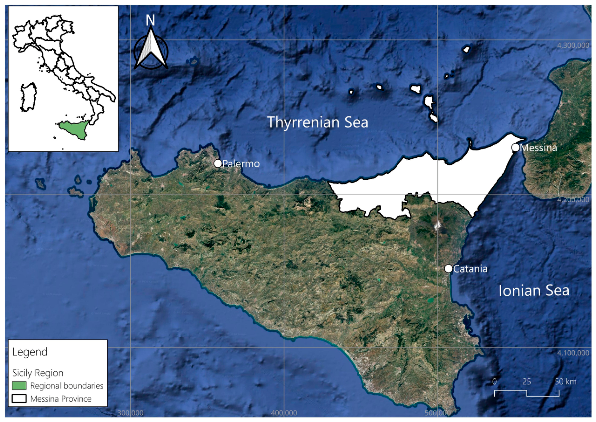
The study area (Figure 1) corresponds to the Metropolitan City of Messina (3247 km²), located in the northeastern sector of Sicily (Italy). This territory represents a strategic Mediterranean junction due to the presence of the Strait of Messina, a highly complex geological and geographical domain. The area extends along the Tyrrhenian and Ionian coasts and includes the mountainous inland regions of the Nebrodi and Peloritani Mountains, which dominate the landscape. The territory is predominantly mountainous and hilly, with a narrow coastal belt, resulting in a complex morphology and high susceptibility to slope instability.

From an orogenetic perspective, the Peloritani Mountains form the southern termination of the Calabrian–Peloritan Arc, a mountain system generated by the convergence and collision between the African plate and a migrated portion of the European plate. This tectonic process produced a complex edifice of superimposed nappes and tectonic slices resulting from plate convergence [42]. The Peloritani chain develops for approximately 65 km from the Strait of Messina to the Etna area. It consists predominantly of metamorphic rocks and is characterized by steep slopes, narrow, deep valleys, and a continuous ridge with average elevations between 800 and 1000 m a.s.l.

The Nebrodi Mountains, in contrast, occupy a large portion of the Apennine–Maghrebide Chain overlooking the Tyrrhenian coast. Developed mainly on arenaceous substrates, this chain extends for about 70 km. It features rounded peaks with extensive summit terraces, almost all exceeding 1500 m a.s.l. (some surpassing 1700 m). From these terraces, valleys open—narrow in the upper reaches and progressively widening toward the coast—furrowed by countless ephemeral streams (“fiumare”) flowing into the Tyrrhenian Sea.

From a hydrogeological perspective, the outcropping terrains exhibit substantial differences in infiltration and water circulation depending on lithology and structural characteristics (fracturing and tectonization). Only one-third of the basin soils present high or medium-high permeability (Metropolitan City of Messina, 2021). From the mountain ridge, numerous torrential watercourses descend on both the Ionian and Tyrrhenian slopes, forming gorges and “fiumare”. The water regime is predominantly seasonal and irregular: the combination of steep slopes and concentrated rainfall can generate sudden flood episodes and debris transport, followed by prolonged low-flow periods [38]. This confirms the primary role of the “fiumare” as the main hydrostructures of the territory, fundamentally shaping the morphological setting and controlling the spatial distribution of hydrogeological hazards.

Vegetation in the Metropolitan City of Messina follows three altitudinal belts following the Pavari classification: the Lauretum (coast to 600–900 m), hosting Mediterranean maquis and agricultural crops (olive groves, citrus orchards, vineyards); the Castanetum (hilly areas), with oak and chestnut woods; and the Fagetum (above 1200 m), characterized by beech and coniferous forests.

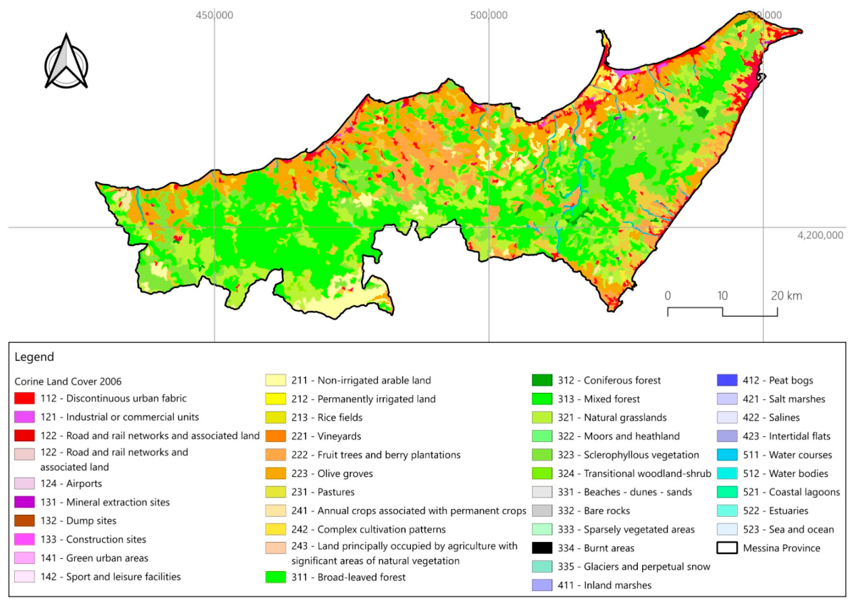
Using the CORINE Land Cover (CLC) map (2006), the Land Use/Land Cover (LULC) configuration is dominated by natural and semi-natural environments, which together constitute the primary land cover categories, followed by agricultural areas and a comparatively smaller but significant artificial footprint. Forests and Semi-natural Areas are the dominant macro-category. Broad-leaved forests represent the primary natural vegetation, covering approximately 24.6% of the area (c. 800 km²) (Figure 2). A very large portion is occupied by transitional woodland-shrub and natural grasslands (approx. 32.8%, c. 1065 km²), highlighting the extensive presence of Mediterranean maquis and garrigue, often the result of land abandonment or fire events.

Despite the mountainous terrain, agricultural land use is relevant, covering about 35.2% (c. 1140 km²). Of this, “Heterogeneous agricultural areas” (including complex cultivation patterns and agriculture with natural vegetation) account for c. 5%, while permanent crops (vineyards, olive groves, fruit trees) represent a significant portion (24.4%, c. 792 km²), reflecting the traditional agricultural economy. A trend of agricultural expansion was observed between 1990 and 2006, particularly in the valley floors, while hillslope and mountain areas showed more complex patterns of abandonment and renaturalisation.

Data from ISPRA (Italian Institute for Environmental Protection and Research) reports indicate a progressive densification of artificial surfaces. Studies on the Italian coastline (2012–2018) show that land consumption continues to increase, with significant pressure within the first 500 m from the sea. In the Metropolitan city of Messina, this leads to the expansion of discontinuous urban fabric along the narrow coastal plains, often encroaching onto alluvial fans and steep slopes, directly interacting with active hydrogeological processes. A critical LULC trend observed in the region is the transformation of forested areas into transitional shrubland or sclerophyllous vegetation. This degradation, often exacerbated by wildfires and unsustainable land management, reduces root cohesion and soil mechanical reinforcement, which are fundamental for slope stability.

The decrease in active agricultural land (specifically complex cultivation patterns and agro-forestry areas) leads to the abandonment of traditional dry-stone terraces. The lack of maintenance on these terraces, which historically acted as hydraulic and retaining structures, increases the susceptibility to shallow landslides and debris flows during high-intensity rainfall events.

During intense and prolonged rainfall events, rapid mass movements affect the regolith and colluvial cover above the bedrock, typically evolving as debris flows and debris avalanches. Consequently, shallow landslides are widespread, involving thixotropic, sandy soils (brown soils, leptic and eutric cambisols) with thicknesses of 50–80 cm, largely controlled by the degree of terrace preservation [43].

The study area has been recurrently struck by destructive rainfall-induced landsliding. Two catastrophic episodes, occurring on 25 March 2007 and 1 October 2009, triggered extensive slope failures that severely damaged rural settlements and road networks surrounding Giampilieri [2,3,4,5,6]. Subsequent events have continued to affect the region in later years, including more recent episodes on both the Ionian and Tyrrhenian flanks:

• 1 March 2011—Ionian side, along the coastal stretch from Messina to Mili.
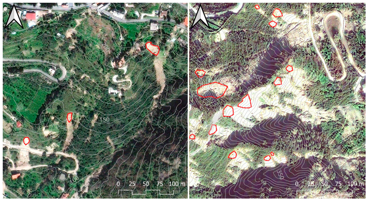
• 9 November 2011—Ionian coast, extending from Messina to Catania (Figure 3).
• 22 November 2011—Tyrrhenian side, from Messina to Barcellona Pozzo di Gotto.
• 2 May 2023—Ionian side, near the municipalities of Antillo and Roccafiorita, in the southern sector of the Messina Metropolitan city.

3. Materials and Methods

The workflow was operationalized using the datasets and procedures described below, all based on open data and free GIS tools. All analyses were carried out in QGIS environment (ver 3.44, QGIS Development Team, 2026) on vector and raster layers, which comprised a Digital Terrain Model, geological and land use/cover maps, soil thickness data, and a landslide inventory. Three experimental free Open Source GIS tools were employed for change detection via raster code differences and for susceptibility assessment using Frequency Ratio, with model reliability evaluated through ROC curves.

3.1. Datasets

The datasets employed in this study originate from three main sources: publicly available online repositories (geology, LULC maps, and DTM); the internal database of ENEA (landslide inventory); and the internal database of CREA (soil thickness data). For each thematic layer, the highest-resolution dataset available for the study area and compatible with the available computational resources was selected.

3.1.1. Digital Terrain Model (DTM)

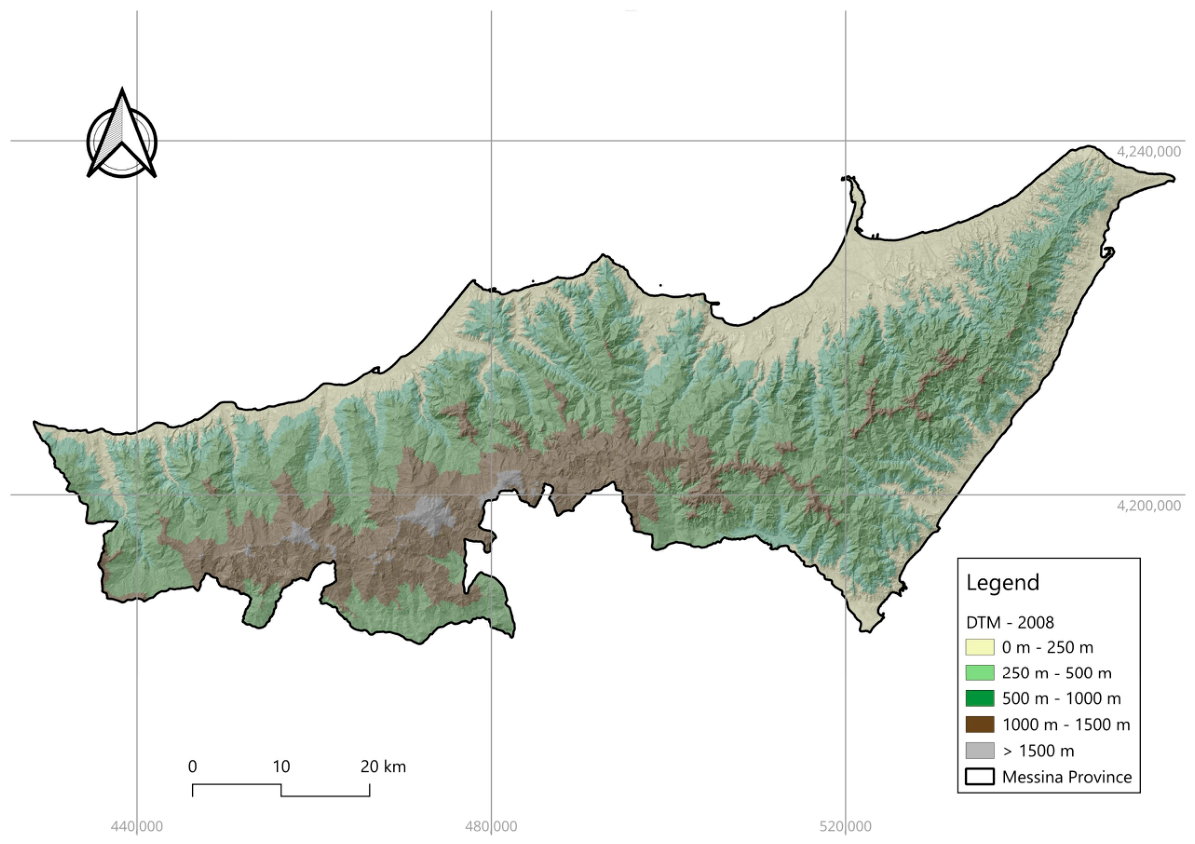
The DTM employed had a 2 m resolution and was acquired in ESRI GRID format, then exported to TIF, in the Gauss–Boaga East reference system (Figure 4). It was generated from aerial images (ATA flight 2004–2008) acquired before the landslide events that affected the Messina area between 2009 and 2011. The original 2 m DTM was resampled to 10 m resolution using bilinear interpolation to ensure computational feasibility for the regional-scale soil thickness modelling and the susceptibility analyses on a standard workstation. Processing the entire study area at 2 m resolution would have required substantially greater computational resources, likely involving HPC infrastructure, which was not available for this study. The 10 m resolution represents a pragmatic compromise between spatial detail and practical operability.

The DTM constitutes the fundamental topographic base from which several morphometric parameters were extracted, including slope angle, aspect, curvature, and topographic wetness index. These parameters are widely recognised as time-independent predisposing factors for shallow landslide initiation.

3.1.2. Lithological Map

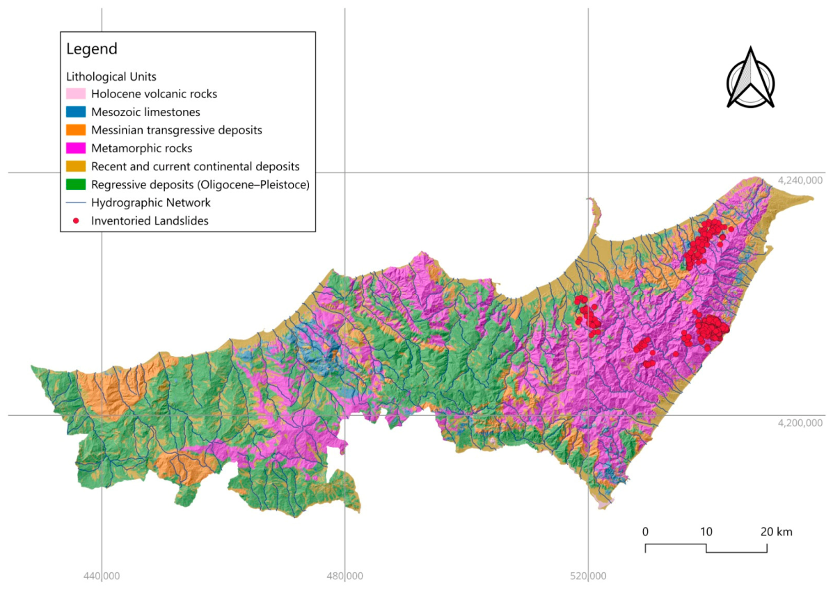
The 1:50,000 geological map (Figure 5) of the Metropolitan City of Messina [44], which provides a detailed lithological and structural characterisation of the outcropping units, was used as a proxy for the geotechnical features of the shallow material covering the bedrock. This is the highest-resolution lithological information currently available at the regional scale for the study area. Although the national CARG project (Geological Mapping of Italy) is producing new 1:50,000 geological sheets, the available tiles do not yet cover the entire Messina province, and their mosaic would have required a complex harmonisation process.

This layer was treated as a time-independent predisposing parameter, as lithological properties remain substantially stable over the temporal scale considered in this study.

3.1.3. Land Use/Land Cover Map (LULC)

The LULC maps used in this study derive from the Corine Land Cover (CLC) programme (https://land.copernicus.eu/en/products/corine-land-cover, accessed on 10 February 2026), the European reference initiative for land cover and land use mapping. CLC production relies on visual interpretation of satellite imagery (Landsat historically, Sentinel-2 more recently) with a 25 ha Minimum Mapping Unit (MMU) and 100 m minimum width for linear features. Limitations include scale dependence on expert interpretation, which have driven the development of higher-resolution products in response to EU policies including the Green Deal, Biodiversity Strategy, and LULUCF. CLC consists of thematic maps (both vector and raster formats) that classify territory according to a three-level hierarchical nomenclature:

• Level 1: 5 main classes (artificial areas, agricultural areas, forests and semi-natural areas, wetlands, water bodies);
• Level 2: 15 intermediate classes derived from Level 1;
• Level 3: 44 detailed classes specifying the 15 intermediate classes.

For the present study, CLC maps from two different time periods (e.g., 1990 and 2006, or the closest available dates) were acquired for the Metropolitan City of Messina. These maps constitute the highest resolution, freely available, and temporally consistent LULC product covering the entire study period and the basis for subsequent temporal variation analysis. The LULC map temporal windows (1990–2006) were intentionally selected as the most recent CORINE Land Cover products available before the landslide events occurred in the area (2007–2011). The subsequent CLC update (2012) would have captured changes occurring after the failures, which could have introduced post event signals into the susceptibility analysis.

It should be noted that the CLC classification system uses numerical codes uniquely associated with each land cover class, a property essential for applying the change detection methodology described in Section 3.2.1.

3.1.4. Soil Thickness Map

Soil thickness is generally considered a fundamental controlling factor in many process-based and statistical slope stability models of shallow landslide initiation [44,45]. In this study, soil depth data were derived from 306 pedological observations (profiles and minipits) within the Messina Metropolitan city, extracted from the national soil database maintained by CREA. Depth was calculated as cumulative soil thickness per site. Spatialization was performed using Digital Soil Mapping techniques, specifically a Random Forest machine learning algorithm implemented in Whitebox Tools (v. 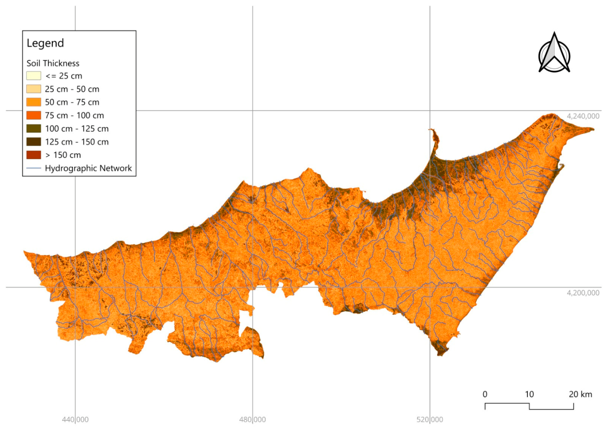2.3.0) [46]. The use of WhiteboxTools allowed the Random Forest regression to be applied efficiently over the entire study area on a standard workstation, thanks to its cluster-based raster processing approach. Predictor covariates included morphometric variables (e.g., slope, curvature, aspect, topographic wetness index) derived from the 10 m DTM (resampled from 2 m LiDAR data), together with a lithology map reclassified into 15 classes. The model was trained on 50% of the points and tested on the remaining 50%. The final output is a 10 m resolution raster map of cumulative soil thickness (min = 19 cm, max = 190 cm; Figure 6). Model performance on the test set yielded an R² of 0.73, an RMSE of approximately 21.95 cm, and a relative RMSE (RRMSE) of 26.71%. The model also shows high performance on the training set (R² = 0.9962), and slope and lithology were identified as the most important predictors. The RRMSE falls within the 20–30% range, which is generally considered “good” for environmental and soil modelling applications, indicating that the error magnitude is well-controlled relative to the mean observed values. The model’s overall predictive capability is therefore statistically robust and suitable for regional-scale spatial analysis.

3.1.5. Shallow Landslide Inventory

A reliable and representative landslide inventory is a fundamental prerequisite for training and validating statistical susceptibility models. A local inventory containing 1200 source areas of debris and mud flows and debris avalanches triggered by heavy rainfall that occurred in the area between 2007 and 2011 was manually compiled. All mapped landslides are located in the north-eastern sector of the study area, within the Peloritani Mountains (Figure 5). In the study area, the mapped source areas have soil depths ranging approximately between 40 cm and 110 cm, and their areal extent is generally between a few tens and a few hundred square metres; only 30 out of 1200 mapped landslides exceed 1000 m². The source areas were identified through field surveys [47] and observation of two high-resolution aerial image datasets. The first was acquired ad hoc after the event of 1 October 2009 by the Civil Protection Department (0.15 m per pixel). The second was derived from QuickBird-02 and GeoEye-01 imagery, orthorectified using an RFM model refined with GCPs and finally produced as orthophotos at 0.5–0.6 m resolution.

The inventory was randomly split into five independent training (80%) and validation (20%) distinct subsets, following standard practice in statistical landslide susceptibility modelling to calibrate the model on independent data and evaluate its predictive performance on unseen cases [48].

3.2. Methods

The methodological framework is organized into three main components, each supported by a dedicated tool or procedure: (i) LULC temporal variation detection using the Raster Code Differences tool; (ii) shallow landslide susceptibility assessment based on Frequency Ratio analysis; (iii) model validation via ROC analysis.

To investigate the relationship between LULC transitions and landslides occurrence, buffer areas were generated around each landslide source area, applying a 1000 m buffer to each source area. Due to the proximity of many source areas (often within 100 m of each other), the resulting buffers overlapped extensively. These overlapping buffers were then dissolved into seven contiguous buffer macro-areas that collectively enclose all 1200 landslide source areas. These seven buffer macro-areas constitute the spatial domain for the calculation of the preliminary landslide indices (LI, LAI) and the preliminary Frequency Ratio analysis on LULC transitions. In contrast, the full susceptibility models (static vs. dynamic LULC) were run on the entire provincial territory (3247 km²), as the objective is to produce spatially exhaustive susceptibility maps.

The study aims to provide a simple, reproducible, and fully GIS-based workflow that can be implemented by technical staff without specific machine learning expertise. The objective was to isolate the effect of LULC transitions on model performance, and the Frequency Ratio method—being transparent and non-parametric—provides an intuitive and interpretable framework for this purpose.

3.2.1. Land Cover Change Detection

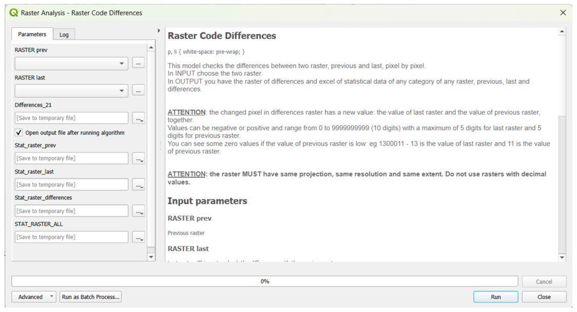
Land cover transitions between 1990 and 2006 were mapped using a post-classification comparison approach. Two CORINE Land Cover (CLC) rasters (t₁ = 1990, t₂ = 2006), sharing the same projection, resolution, and nomenclature, were processed through the Raster Code Differences (RCD) tool (available at https://github.com/geohaze24/Raster-Code-Differences, accessed on 31 July 2026). The RCD tool (Figure 7) concatenates the numerical codes of each class at the two-time steps, generating a transition raster where each unique pair (code_t₁, code_t₂) identifies a specific land cover trajectory. For each pixel, the operation compares the two LULC rasters: if the values are equal (no change), the original value is retained; otherwise, the two numerical codes are combined into a single ten-digit identifier by multiplying the earlier code by 100,000 and adding the later code. This yields a transition raster where each unique pair of codes identifies a specific LULC trajectory between the two-time steps. The RCD output is a transition map that captures where and how land cover changed over the 18-year period.

3.2.2. Susceptibility Modelling with Static and Dynamic LULC

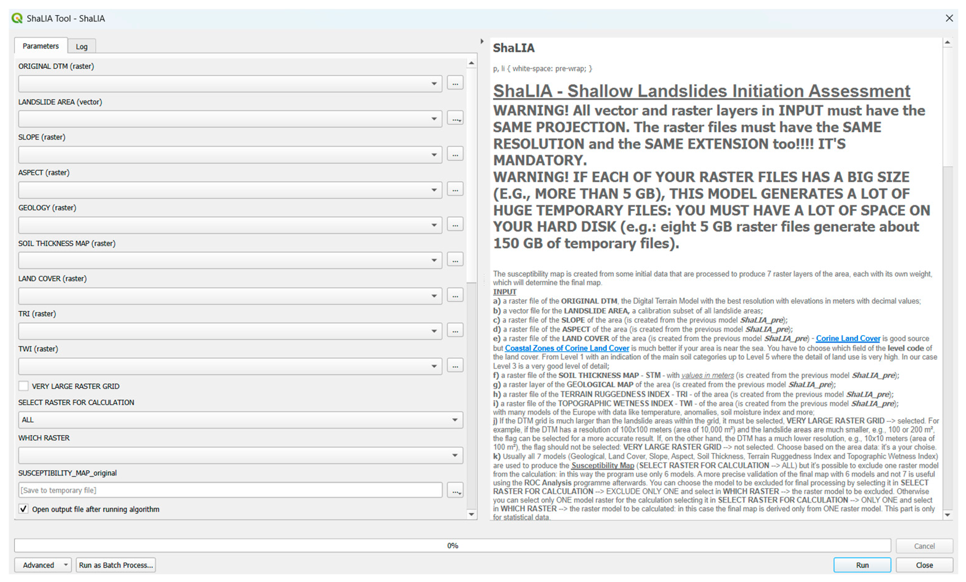
Shallow landslide susceptibility was assessed using the Frequency Ratio (FR) method, implemented in the Shallow Landslide Initiation Assessment (ShaLIA) tool (available at https://github.com/geohaze24/ShaLIA, accessed on 31 July 2026; Figure 8) that computes bivariate statistical susceptibility indices—including Frequency Ratio—together with ROC-based validation, for shallow-landslide initiation susceptibility mapping. For each class $i$ of a given conditioning factor, FR is computed as:

$$I_{jk}={FR}_{jk}={\displaystyle \frac{\raisebox{1ex}{${Landslide}_{jk}$}\!\left/ \!\raisebox{-1ex}{${Landslide}_{tot}$}\right.}{\raisebox{1ex}{${Area}_{jk}$}\!\left/ \!\raisebox{-1ex}{${Area}_{tot}$}\right.}}$$

(1)

where

• Landslide_jk indicates the sum of the cells of class k of parameter j within the polygons of the landslide areas;
• Landslide_tot indicates the sum of all the polygons of the landslide areas;
• Area^jk is the sum of all the areas of a certain class k of parameter j;
• Area^tot is the entire study area extent.

$F{R}_{jk}>1$ indicates a class more prone to landsliding than average and the final susceptibility index (LSI) is the pixel-wise sum of FR values across all factors.

Two model configurations were compared:

• Static model: includes LULC as a time-independent factor, using the 2006 CLC map.
• Dynamic model: replaces the static LULC map with the 1990–2006 transition map. All other predisposing factors (slope, aspect, lithology, soil thickness) remain identical between the two configurations.

For each configuration, five runs were performed with the five calibration subsets (80% of the landslide inventory).

3.2.3. Model Validation (ROC Analysis)

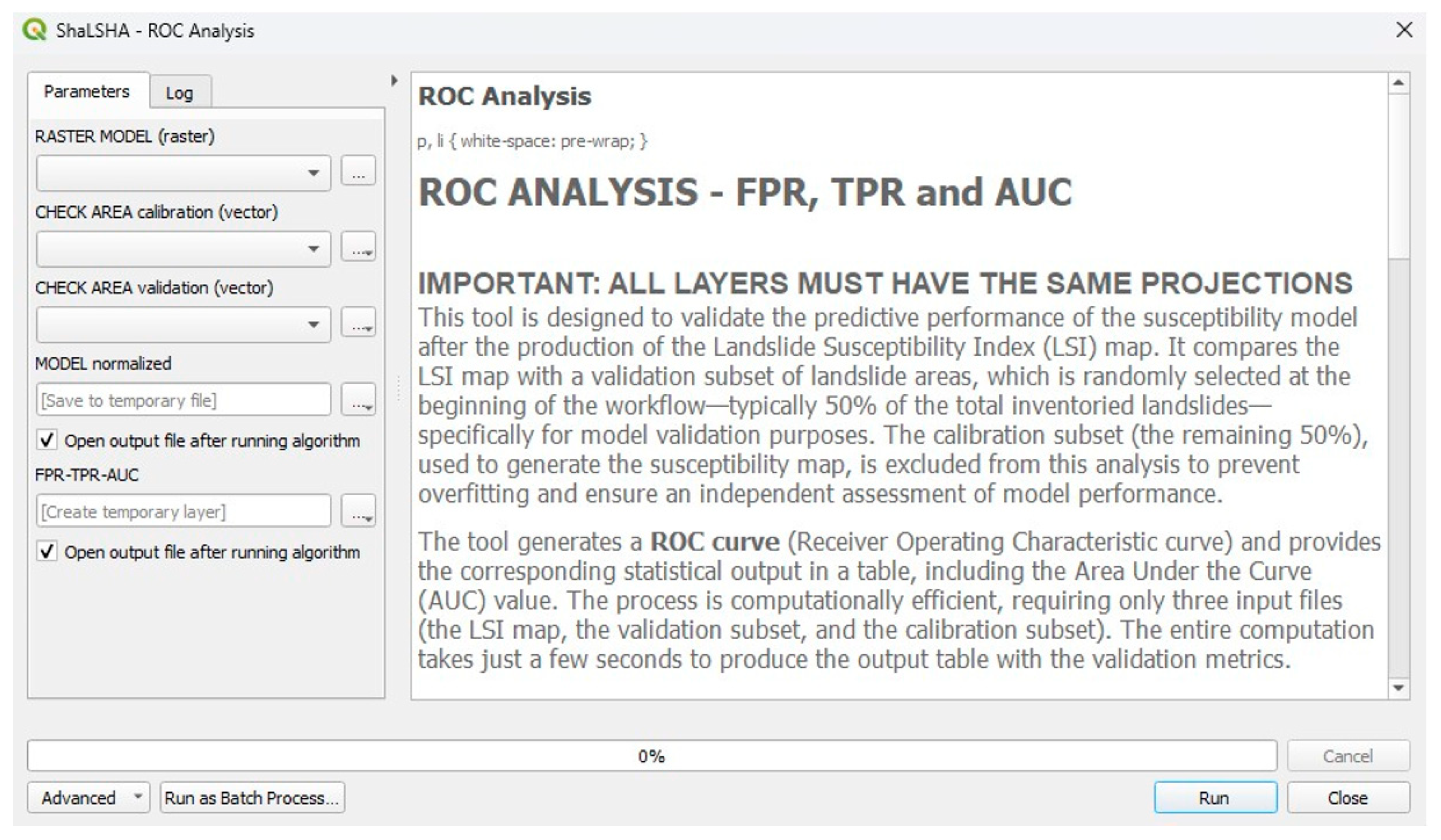
Predictive performance was evaluated using the validation subset (20% of the landslide inventory) and Receiver Operating Characteristic (ROC) analysis with a specific GIS tool (available at the same link of ShaLIA; Figure 9).

ROC analysis is a standard method for binary classifiers (landslide presence/absence; [49]). The ROC curve plots the True Positive Rate against the False Positive Rate across all classification thresholds, providing a threshold-independent assessment of model performance [50,51,52]. The Area Under the Curve (AUC) summarises the model’s discriminative ability; values between 0.7 and 0.9 are generally considered indicative of good performance [53].

The Area Under the Curve (AUC) was computed for both the static and dynamic models. The AUC provides a threshold-independent measure of model discriminative ability, ranging from 0.5 (random performance) to 1.0 (perfect discrimination).

4. Results

The results are organised in three parts. First, LULC transitions observed in the Metropolitan City of Messina between 1990 and 2006 (Figure 10) are summarised at the provincial scale. Second, the same transitions are analysed within the seven buffer macro-areas, where two landslide indices (LI and LAI) and a preliminary Frequency Ratio (FR) on LULC transitions are computed. Third, the full susceptibility models (static vs. dynamic LULC) are compared across the entire provincial territory, using ROC analysis validation.

4.1. Provincial-Scale LULC Transitions (1990–2006)

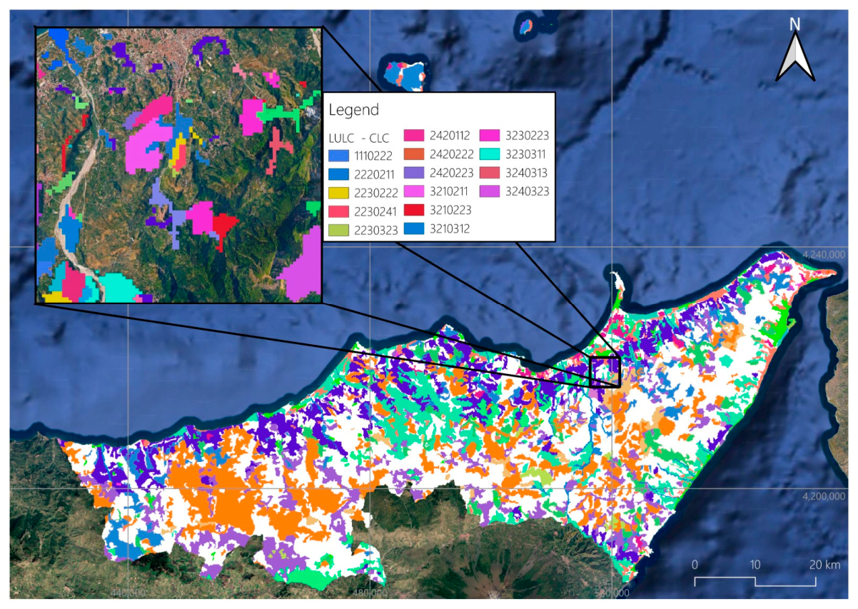
The comparison of CLC maps from 1990 and 2006 for the entire Metropolitan City of Messina reveals broad patterns of land cover change (box in Figure 11). These patterns serve as an exploratory context for the subsequent local-scale analyses.

This map is illustrative rather than exhaustive: it shows the full provincial-scale transition raster, with a zoomed inset highlighting a representative subset of transition codes for legibility.

Table 1. Variations and invariations of artificial surfaces (m²).

Corine Land Cover	Code	CLC 1990	Invariation	Acquired	Lost	Acquired—Lost
Continuous urban fabric	111	52,430,000	42,920,000	3,870,000	9,510,000	−5,640,000
Discontinuous urban fabric	112	111,460,000	81,230,000	17,830,000	30,230,000	−12,400,000
Industrial or commercial units	121	11,830,000	7,340,000	2,630,000	4,490,000	−1,860,000
Road and rail networks and associated land	122	3,540,000	1,130,000	380,000	2,410,000	−2,030,000
Port areas	123	2,140,000	1,520,000	230,000	620,000	−390,000
Mineral extraction sites	131	5,940,000	3,600,000	250,000	2,340,000	−2,090,000
Construction sites	133	450,000	-	-	450,000	−450,000
Sport and leisure facilities	142	300,000	-	-	300,000	−300,000

,

Table 2. Variations and invariances of agricultural areas (m²).

Corine Land Cover	Code	CLC 1990	Invariation	Acquired	Lost	Acquired—Lost
Non-irrigated arable land	211	82,090,000	73,120,000	53,550,000	8,970,000	44,580,000
Fruit trees and berry plantations	222	267,350,000	218,700,000	45,940,000	48,650,000	−2,710,000
Olive groves	223	389,700,000	337,970,000	69,250,000	51,730,000	17,520,000
Annual crops associated with permanent crops	241	18,930,000	7,960,000	13,410,000	10,970,000	2,440,000
Complex cultivation patterns	242	56,910,000	37,690,000	30,810,000	19,220,000	11,590,000
Land principally occupied by agriculture, with significant areas of natural vegetation	243	189,240,000	116,180,000	92,240,000	73,060,000	19,180,000

and

Table 3. Variations and invariances of forest and semi-natural vegetation (m²).

Corine Land Cover	Code	CLC 1990	Invariation	Acquired	Lost	Acquired—Lost
Broad-leaved forest	311	586,540,000	510,210,000	334,290,000	76,330,000	257,960,000
Coniferous forest	312	14,970,000	8,270,000	5,160,000	6,700,000	−1,540,000
Mixed forest	313	91,660,000	56,900,000	45,800,000	34,760,000	11,040,000
Natural grasslands	321	444,000,000	282,300,000	153,580,000	161,700,000	−8,120,000
Moors and heathland	322	195,270,000	-	-	195,270,000	−195,270,000
Sclerophyllous vegetation	323	344,300,000	201,560,000	322,880,000	142,740,000	180,140,000
Transitional woodland-shrub	324	297,620,000	15,620,000	5,820,000	282,000,000	−276,180,000
Beaches, dunes, sands	331	910,000	390,000	230,000	520,000	−290,000
Bare rocks	332	14,220,000	7,040,000	920,000	7,180,000	−6,260,000
Sparsely vegetated areas	333	29,130,000	-	-	29,130,000	−29,130,000

report the complete area-based statistics for the artificial, agricultural, and forest/semi-natural macro-categories at the provincial scale, while

Table 4. Variations (xxx to yyy) in buffer areas by number of pixels and by area. Each analyzed pixel represents an area of 10,000 m².

Variations	Pixel	Variations	Pixel	Variations	Pixel	Variations	Pixel
111 to 223	28	223 to 243	7	322 to 243	322	324 to 313	12
112 to 111	23	223 to 323	10	322 to 311	3	324 to 321	10
112 to 222	52	243 to 223	21	322 to 321	202	324 to 323	163
112 to 223	45	243 to 321	136	322 to 323	18	333 to 243	37
112 to 311	5	311 to 313	152	323 to 112	3	333 to 321	83
112 to 323	15	311 to 323	1	323 to 222	7	333 to 323	7
131 to 223	5	312 to 313	123	323 to 223	164	511 to 222	5
222 to 211	4	313 to 223	52	323 to 243	19
222 to 243	12	321 to 211	27	323 to 311	132
222 to 311	6	321 to 223	65	323 to 313	53
223 to 222	21	321 to 311	12	323 to 321	66
223 to 241	18	321 to 323	426	324 to 311	42

and

Table 5. Final class of variation in buffer areas (m² and pixel).

Codes	Area (m2)	Pixel
111	230,000	23
112	30,000	3
211	310,000	31
222	850,000	85
223	3,800,000	380
241	180,000	18
243	3,970,000	397
311	2,000,000	200
313	3,400,000	340
321	4,970,000	497
323	6,400,000	640

report the transitions occurring specifically within the seven buffer macro-areas (Section 4.2).

Artificial surfaces show an apparent decrease (Table 1). This is largely attributable to the scale limitations of CLC (MMU of 25 ha) and to methodological inconsistencies between editions, rather than to actual urban contraction.

Agricultural areas show an apparent increase (Table 2), reflecting the progressive reclassification of hybrid landscapes (e.g., abandoned terraced areas) from transitional vegetation into agricultural categories, particularly into class 243 (“areas predominantly occupied by agriculture with significant natural spaces”).

Forest and semi-natural vegetation show no net growth trend (Table 3), due to the slow pace of ecological succession and difficulties in discriminating between sparse forest, Mediterranean maquis, and evolving vegetation. Sclerophyllous vegetation (class 323) increases systematically as a stable intermediate stage of renaturalisation.

4.2. Transitions Within Buffer Macro-Areas and Landslide Source Areas

The analysis of the LULC variations was performed on the seven buffer macro-areas (each obtained by dissolving overlapping 1 km buffers around the 1200 landslide source areas). These macro-areas represent the local morphological context comparable to the landslide sites. The analysis evidences each variation typology (Table 4) and the extension in pixels and square meters of the final classes (Table 5).

Within these buffers, four transition classes dominate the landslide source areas. Class 243 (areas predominantly occupied by agriculture with significant natural spaces) and class 321 (natural grasslands and pastures) each account for 66 landslide events. Class 323 (sclerophyllous vegetation) accounts for 37 events, and class 311 (broad-leaved forests) for 31 events. Classes 243 and 321 deviate most strongly from the provincial trend, suggesting a systematic association with landslide-prone settings.

4.3. Landslide Indices Within Buffer Macro-Areas

To enable comparison among classes with different areal extents, two indices were computed within the buffer macro-areas. The Landslide Index (LI), defined as the number of landslide events divided by the area of the class in square metres, yields low and relatively homogeneous values across classes. The Areal Landslide Index (LAI), defined as the area of the class within source areas divided by the total area of all source areas, shows strong variability.

Landslides are concentrated in the four classes identified above, which collectively occupy a large portion of the buffer macro-areas. Consequently, LAI is high for these classes: 36.7 for class 323 (sclerophyllous vegetation), 26.8 for class 321 (natural grasslands and pastures), 19.7 for class 243 (agriculture with significant natural spaces), and 11.0 for class 311 (broad-leaved forests). This indicates that landslide distribution broadly mirrors the landscape structure within the buffers.

Several minor classes (e.g., orchards, arable land, mixed forests) show elevated LI values despite very few landslide events. These are interpreted as statistical spikes due to limited areal extent and possible classification errors, not as genuine susceptibility indicators.

4.4. Preliminary Frequency Ratio on LULC Transitions (Within Buffer Macro-Areas)

This preliminary FR analysis is specific to LULC transitions and is computed within the seven buffer macro-areas. Its purpose is to diagnose whether dynamic LULC information is associated with landslide occurrence, before running the full susceptibility model.

For static LULC classes (2006) within buffer macro-areas, four classes have FR greater than 1, indicating over-representation in landslide source areas relative to the buffer macro-areas. Class 323 (sclerophyllous vegetation) has an FR of 1.48, class 311 (broad-leaved forests) 1.42, class 321 (natural grasslands and pastures) 1.40, and class 243 (agriculture with significant natural spaces) 1.28. These classes typically occupy hilly or mountain slopes with thin soils and discontinuous vegetation cover—conditions that favour shallow landslide initiation.

For LULC transitions (dynamic information), the preliminary analysis suggests that certain transition trajectories are more strongly associated with landsliding than static end-state classes alone, motivating the full model comparison.

4.5. Susceptibility Models on the Entire Provincial Territory

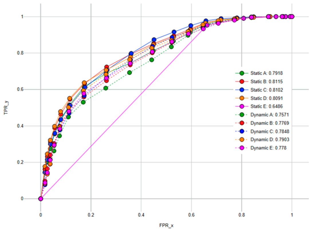
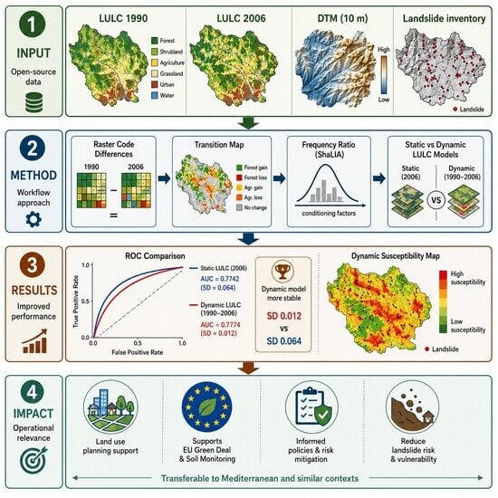
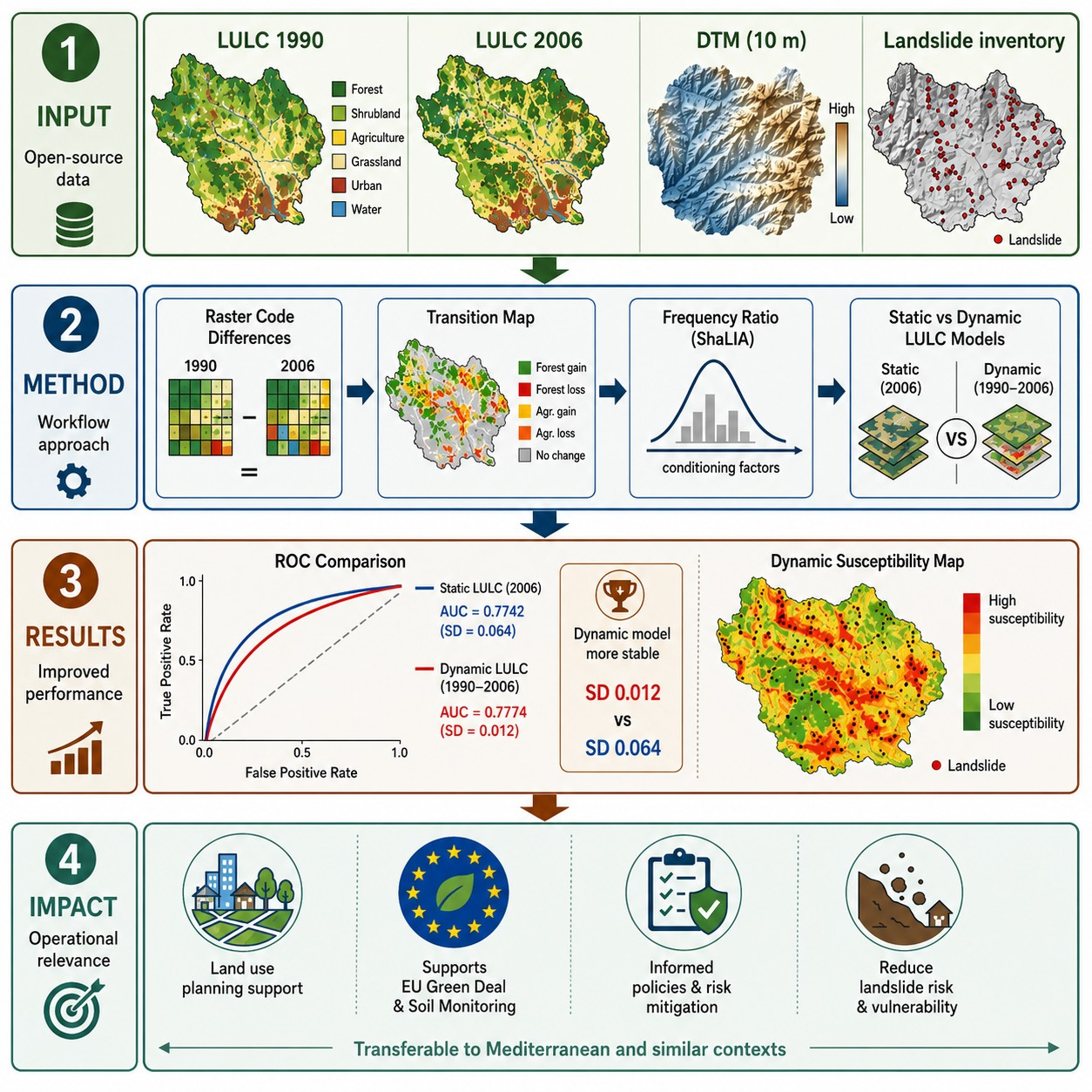
The two susceptibility models were compared using five independent random splits of the landslide inventory (80% for training, 20% for validation). For each split, the static and dynamic LULC models were calibrated on the training subset, and the resulting LSI maps were validated on the corresponding validation subset using a GIS-based ROC analysis tool (Figure 11). The two models yielded very similar mean AUC values (static = 0.7742; dynamic = 0.7774), with a difference of only 0.0032. However, their stability across splits differs markedly, as evidenced by the standard deviation values: static SD = 0.064; dynamic SD = 0.012. This pattern arises because the static model performs well on four splits (AUC > 0.79) but drops sharply on split E (AUC = 0.6486). The dynamic model shows more consistent behaviour, with all AUC values falling within a narrow range (0.757–0.790) and no extreme low values.

5. Discussion

The datasets used in this study are the highest-resolution products that could be reasonably handled for the Messina province. The soil thickness map, in particular, was produced explicitly for the landslide hazard purpose because no public-domain product exists at a comparable resolution. Although the RMSE (~22 cm) highlights a non-negligible error when compared to the typical shallow soil thickness in the area (50–80 cm), this level of error is not unusual for spatially distributed soil depth products derived from point observations, especially in complex mountainous terrain. The alternative—using a uniform soil depth or simplified empirical models (e.g., the Z or S models by Saulnier et al., 1997 [54])—would introduce even greater and less constrained uncertainty.

Although a public inventory is available from the regional geoportal and the IdroGEO portal (ISPRA; https://idrogeo.isprambiente.it/app/, accessed on 31 July 2026), it is considerably less complete than the locally compiled inventory. Moreover, it consists of polygons that include the entire landslide body (source, transport, and accumulation areas), without distinguishing the source areas alone. This would have introduced significant uncertainty in the susceptibility analysis, as the Frequency Ratio approach requires precise identification of the initiation zones.

The preliminary analysis within the seven buffer macro-areas suggested that LULC transitions might influence shallow landslide occurrence, providing higher landslide indices (LI, LAI) and higher preliminary Frequency Ratios. This motivated the comparison between static and dynamic LULC configurations in the full susceptibility model. However, when applied to the entire provincial territory, the expected improvement in mean AUC did not materialise: the dynamic model achieved a mean AUC (0.7774) almost identical to the static one (0.7742).

What did emerge was a difference in the distribution of AUC values across the five random splits. The static model performed well on four splits (AUC > 0.79) but showed a single markedly lower value on split E (AUC = 0.6486). The dynamic model showed no extreme low values, with all AUCs falling within a narrow range (0.757–0.790). This pattern could indicate greater stability of the dynamic model, although the difference is largely attributable to the anomalous split E. With a larger number of splits (e.g., 50 or 100), the impact of a single anomalous partition would likely be attenuated. This observation should therefore be considered preliminary.

While the mean AUC values are nearly identical, the standard deviation differs markedly (0.064 vs. 0.012), suggesting that the dynamic model is less sensitive to the specific composition of the training/validation partition. This aspect of model robustness has received less attention in the recent LULC–landslide literature, which has largely focused on maximising predictive accuracy. For operational susceptibility mapping—where the exact composition of the training set cannot be controlled—robustness may be as important as peak performance.

Recent works have adopted more sophisticated machine learning techniques (XGBoost, Random Forest, SHAP) to address the LULC–landslide relationship from complementary perspectives. Hu et al. (2025) [55] introduced sediment connectivity as an additional dynamic factor in the Three Gorges Reservoir area. Pratama et al. (2026) [56] provided a detailed morphometric characterisation of landslides across different LULC types in a tropical mountain watershed. Xia et al. (2026) [57] reconstructed LULC transition pathways (Disturbance → Degradation → Reconstruction) in a mountainous urban region of China. These approaches typically treat LULC as a static predictor or as an input to future scenario modelling, without explicitly comparing static versus dynamic configurations. In contrast, the present study isolates the effect of LULC transitions by keeping all other predisposing factors identical between two model runs. In some cases, these studies achieved high AUC values, often exceeding 0.90 over large areas [58,59], higher than those obtained here. Nevertheless, a direct comparison of AUC values must be made with caution. Studies reporting very high AUCs often include deep-seated rotational and translational slides, which are typically characterised by recurrence in the same or adjacent areas. In such contexts, a high AUC is expected. The present study focuses exclusively on rainfall-triggered shallow landslides (debris flows, debris avalanches), which are predominantly newly formed events. Unlike deep-seated slides, shallow landslides typically occur in areas without previous slope failures. A very high AUC (>0.90) would therefore be geomorphologically less plausible for shallow landslide susceptibility. Moderate AUC values (0.75–0.85) are more realistic and should be interpreted as a correct representation of the inherent spatial variability of shallow landslide initiation.

The only study conducted in a comparable Mediterranean setting (Briga catchment, within the same Metropolitan city of Messina) is that of Reichenbach et al. (2014) [60]. Using land use maps from 1954 and 2009 and a slope-unit-based multivariate approach, they showed that expansion of bare soil at the expense of forested areas increased landslide susceptibility. Our results, obtained with a different method (pixel-based FR, random splits, ROC) and over a larger area, are consistent with their findings. This convergence reinforces the robustness of the observation across different modelling techniques.

Several limitations must be acknowledged, most of which are related to the scale mismatch between the different input layers—a factor that may have limited the AUC improvement of the dynamic model. The CORINE Land Cover dataset has an inherently coarse spatial resolution (cell size 100 m, MMU 25 ha) compared to the 10 m resolution of the DTM and the typical size of shallow landslides source in the study area, typically smaller than 1000 m²—one order of magnitude smaller than a single CLC cell. This mismatch, a typical Modifiable Areal Unit Problem example (MAUP) [61], may lead to under-representation of critical LULC transitions, particularly at the scale of individual hillslope terraces, road cuts or small-scale deforestation—which may be critical for slope stability but are either averaged out or misclassified within the CLC raster. The resulting scale mismatches between the coarser LULC and the finer DTM and STM are therefore not due to an arbitrary choice, but rather reflect the current limits of data availability in the study area. Future work with higher-resolution LULC (e.g., Sentinel-2 based classifications at 10 m) could help to better capture these fine-scale processes.

Second, the number of random splits (five) is limited. A larger number of iterations or a full k-fold cross-validation would provide more stable estimates. Third, the analysis does not account for the temporal lag between land use change and slope stability. Future work with more frequently updated LULC products (e.g., annual or biennial classifications) could better capture pre-event changes and reduce the temporal mismatch.

6. Conclusions

The complex geological, geomorphological and vegetation configuration of the Metropolitan City of Messina makes the territory particularly vulnerable to shallow landslides, which have historically caused extensive damage and loss of life. Understanding the interactions between natural processes and anthropogenic transformations of the territory—the subject of this study—is therefore crucial for risk prevention and management.

Land cover is not a static parameter but a dynamic factor, and its temporal evolution influences slope stability. Traditional susceptibility models that treat LULC as invariant may therefore underestimate or misrepresent susceptibility in rapidly changing landscapes. This study developed a methodological framework to quantify the influence of multi-temporal LULC changes on shallow landslide initiation and to incorporate this information into susceptibility mapping. The workflow, based entirely on open data and free GIS tools, integrates three components: (i) detection of LULC temporal variations using the Raster Code Differences tool; (ii) susceptibility assessment tool with Frequency Ratio; (iii) model validation through ROC analysis.

The preliminary analysis within buffer macro-areas, based on the LI and LAI indices, suggested a clearer role of LULC transitions in landslide occurrence. In the study area, heterogeneous agricultural landscapes (class 243), natural grasslands (321), and sclerophyllous vegetation (323) deserve particular attention, as they combine morphological predisposition with land cover characteristics that appear to favour shallow landslide initiation.

Nevertheless, incorporating LULC transitions into the susceptibility model at the provincial scale did not increase the mean AUC compared to a static LULC configuration (0.7774 vs. 0.7742). Across the five random splits, the dynamic model showed a more regular distribution of AUC values than the static model, although the difference is largely driven by a single anomalous split in the static configuration and should therefore be considered preliminary. Overall, the AUC values obtained for both configurations were stable and fell within the 0.75–0.85 range, which is generally considered realistic for shallow landslide susceptibility models. The scale mismatch between the LULC data and the other input layers may partly explain the limited AUC improvement of the dynamic model.

The patterns observed in the buffer-scale analysis suggest a potential role of certain LULC transitions, but this hypothesis requires further investigation before it can inform land planning decisions.

Future research should explore: (i) higher-resolution LULC products (e.g., Sentinel-2 based classifications at 10 m) to capture fine-scale processes; (ii) a larger number of random splits or a full k-fold cross-validation design to confirm the observed pattern of reduced variability; (iii) integration of LULC transitions into machine learning models (e.g., Random Forest, XGBoost) to assess whether the observed stability advantage is preserved; (iii) explicit modelling of time lags between land use change and landslide response to account for the delayed effects of vegetation loss, soil degradation, and changes in subsurface hydrology on slope stability;

Finally, the objectives of this study are consistent with recent European policies (Green Deal, Biodiversity Strategy, Soil Monitoring Law) that emphasise the need to monitor land use changes and their effects on environmental hazards. If the observed patterns are confirmed and strengthened by further studies, incorporating LULC transitions into susceptibility models could help move beyond the static approaches that still dominate the literature, towards more dynamic and temporally aware landslide hazard assessments.

References

- Froude, M.J.; Petley, D.N. Global Fatal Landslide Occurrence from 2004 to 2016. Nat. Hazards Earth Syst. Sci. 2018, 18, 2161–2181. [Google Scholar] [CrossRef] [Scilit]
- Aronica, G.T.; Brigandí, G.; Morey, N. Flash Floods and Debris Flow in the City Area of Messina, North-East Part of Sicily, Italy in October 2009: The Case of the Giampilieri Catchment. Nat. Hazards Earth Syst. Sci. 2012, 12, 1295–1309. [Google Scholar] [CrossRef] [Scilit]
- Casalbore, D.; Chiocci, F.L.; Scarascia Mugnozza, G.; Tommasi, P.; Sposato, A. Flash-Flood Hyperpycnal Flows Generating Shallow-Water Landslides at Fiumara Mouths in Western Messina Strait (Italy). Mar. Geophys. Res. 2011, 32, 257–271. [Google Scholar] [CrossRef] [Scilit]
- Ardizzone, F.; Basile, G.; Cardinali, M.; Casagli, N.; Del Conte, S.; Del Ventisette, C.; Fiorucci, F.; Garfagnoli, F.; Gigli, G.; Guzzetti, F.; et al. Landslide Inventory Map for the Briga and the Giampilieri Catchments, NE Sicily, Italy. J. Maps 2012, 8, 176–180. [Google Scholar] [CrossRef] [Scilit]
- Fiorillo, F.; Diodato, N.; Meo, M.; Mauro, P. Landslides and Flash Floods Induced by the Storm of 22nd November 2011 in Northeastern Sicily. Environ. Earth Sci. 2018, 77, 602. [Google Scholar] [CrossRef] [Scilit]
- Ciampalini, A.; Raspini, F.; Bianchini, S.; Frodella, W.; Bardi, F.; Lagomarsino, D.; Di Traglia, F.; Moretti, S.; Proietti, C.; Pagliara, P.; et al. The Landslide Geodatabase of the Messina Province: A Tool in the Civil Protection Emergency Cycle. Rendiconti Online Della Soc. Geol. Ital. 2015, 35, 70–73. [Google Scholar] [CrossRef] [Scilit]
- Varnes, D.J. Landslide Hazard Zonation: A Review of Principles and Practice; Natural Hazards; Unesco: Paris, France, 1984. [Google Scholar]
- Dikau, R. (Ed.) Landslide Recognition: Identification, Movement and Courses; Publication/International Association of Geomorphologists; Reprinted; Wiley: Chichester, UK, 1997. [Google Scholar]
- Hungr, O.; Leroueil, S.; Picarelli, L. The Varnes Classification of Landslide Types, an Update. Landslides 2014, 11, 167–194. [Google Scholar] [CrossRef] [Scilit]
- Tyagi, A.; Kamal Tiwari, R.; James, N. A Review on Spatial, Temporal and Magnitude Prediction of Landslide Hazard. J. Asian Earth Sci. X 2022, 7, 100099. [Google Scholar] [CrossRef] [Scilit]
- Shano, L.; Raghuvanshi, T.K.; Meten, M. Landslide Susceptibility Evaluation and Hazard Zonation Techniques—A Review. Geoenviron. Disasters 2020, 7, 18. [Google Scholar] [CrossRef] [Scilit]
- Donnini, M.; Bucci, F.; Santangelo, M.; Cardinali, M.; Reichenbach, P. The Effect of Different Landslide Mapping Approaches on the Geomorphological Assessment of Landslide Hazard. EGUsphere 2025, 2025, 1–38. [Google Scholar] [CrossRef] [Scilit]
- Rickenmann, D. Debris-Flow Hazard Assessment and Methods Applied in Engineering Practice. Int. J. Eros. Control Eng. 2016, 9, 80–90. [Google Scholar] [CrossRef] [Scilit]
- Reichenbach, P.; Rossi, M.; Malamud, B.D.; Mihir, M.; Guzzetti, F. A Review of Statistically-Based Landslide Susceptibility Models. Earth-Sci. Rev. 2018, 180, 60–91. [Google Scholar] [CrossRef] [Scilit]
- Berti, M.; Pizziolo, M.; Scaroni, M.; Generali, M.; Critelli, V.; Mulas, M.; Tondo, M.; Lelli, F.; Fabbiani, C.; Ronchetti, F.; et al. RER2023: The Landslide Inventory Dataset of the May 2023 Emilia-Romagna Meteorological Event. Earth Syst. Sci. Data 2025, 17, 1055–1074. [Google Scholar] [CrossRef] [Scilit]
- Ado, M.; Amitab, K.; Maji, A.K.; Jasińska, E.; Gono, R.; Leonowicz, Z.; Jasiński, M. Landslide Susceptibility Mapping Using Machine Learning: A Literature Survey. Remote Sens. 2022, 14, 3029. [Google Scholar] [CrossRef] [Scilit]
- Baiocchi, V.; Vatore, F.; Lombardi, M.; Monti, F.; Onori, R. The Contribution of Open-Source GIS Software and Open Spatial Data for the Re-Evaluation of Landslide Risk and Hazard in View of Climate Change. Geogr. Tech. 2021, 16, 153–162. [Google Scholar] [CrossRef] [Scilit]
- Trigila, A.; Iadanza, C.; Romeo, S.; Di Paola, G.; Gambino, P.; Calcaterra, S.; Zastrow, L.R.; Romano, D.; Biondo, T.; Noman, M.; et al. Advancing Landslide Knowledge and Dissemination in Italy through IdroGEO 2.0 Web Platform. Landslides 2026, 23, 477–487. [Google Scholar] [CrossRef] [Scilit]
- Chen, X.; Li, W.; Hsu, C.-Y.; Arundel, S.T.; Higman, B. Harnessing Geospatial Artificial Intelligence and Deep Learning for Landslide Inventory Mapping: Advances, Challenges, and Emerging Directions. Remote Sens. 2025, 17, 1856. [Google Scholar] [CrossRef] [Scilit]
- Casagli, N. An Inventory-Based Approach to Landslide Susceptibility Assessment and Its Application to the Virginio River Basin, Italy. Environ. Eng. Geosci. 2004, 10, 203–216. [Google Scholar] [CrossRef] [Scilit]
- Fiorucci, M.; Martino, S.; Bozzano, F.; Prestininzi, A. Comparison of Approaches for Data Analysis of Multi-Parametric Monitoring Systems: Insights from the Acuto Test-Site (Central Italy). Appl. Sci. 2020, 10, 7658. [Google Scholar] [CrossRef] [Scilit]
- Gunzburger, Y.; Merrien-Soukatchoff, V.; Guglielmi, Y. Influence of Daily Surface Temperature Fluctuations on Rock Slope Stability: Case Study of the Rochers de Valabres Slope (France). Int. J. Rock Mech. Min. Sci. 2005, 42, 331–349. [Google Scholar] [CrossRef] [Scilit]
- Weidinger, J.T.; Schramm, J.-M.; Surenian, R. On Preparatory Causal Factors, Initiating the Prehistoric Tsergo Ri Landslide (Langthang Himal, Nepal). Tectonophysics 1996, 260, 95–107. [Google Scholar] [CrossRef] [Scilit]
- Delchiaro, M.; Della Seta, M.; Martino, S.; Moumeni, M.; Nozaem, R.; Marmoni, G.M.; Esposito, C. The Role of Long-Term Preparatory Factors in Mass Rock Creep Deforming Slopes: Insights from the Zagros Mts. Belt (Iran). Landslides 2024, 21, 1735–1755. [Google Scholar] [CrossRef] [Scilit]
- Grämiger, L.M.; Moore, J.R.; Gischig, V.S.; Loew, S. Thermomechanical Stresses Drive Damage of Alpine Valley Rock Walls During Repeat Glacial Cycles. J. Geophys. Res. Earth Surf. 2018, 123, 2620–2646. [Google Scholar] [CrossRef] [Scilit]
- Pacheco Quevedo, R.; Velastegui-Montoya, A.; Montalván-Burbano, N.; Morante-Carballo, F.; Korup, O.; Daleles Rennó, C. Land Use and Land Cover as a Conditioning Factor in Landslide Susceptibility: A Literature Review. Landslides 2023, 20, 967–982. [Google Scholar] [CrossRef] [Scilit]
- Knevels, R.; Petschko, H.; Proske, H.; Leopold, P.; Mishra, A.N.; Maraun, D.; Brenning, A. Assessing Uncertainties in Landslide Susceptibility Predictions in a Changing Environment (Styrian Basin, Austria). Nat. Hazards Earth Syst. Sci. 2023, 23, 205–229. [Google Scholar] [CrossRef] [Scilit]
- Gariano, S.L.; Petrucci, O.; Rianna, G.; Santini, M.; Guzzetti, F. Impacts of Past and Future Land Changes on Landslides in Southern Italy. Reg. Environ. Change 2018, 18, 437–449. [Google Scholar] [CrossRef] [Scilit]
- Pepe, G.; Mandarino, A.; Raso, E.; Scarpellini, P.; Brandolini, P.; Cevasco, A. Investigation on Farmland Abandonment of Terraced Slopes Using Multitemporal Data Sources Comparison and Its Implication on Hydro-Geomorphological Processes. Water 2019, 11, 1552. [Google Scholar] [CrossRef] [Scilit]
- García-Ruiz, J.M.; Beguería, S.; Alatorre, L.C.; Puigdefábregas, J. Land Cover Changes and Shallow Landsliding in the Flysch Sector of the Spanish Pyrenees. Geomorphology 2010, 124, 250–259. [Google Scholar] [CrossRef] [Scilit]
- Guo, Z.; Ferrer, J.V.; Hürlimann, M.; Medina, V.; Puig-Polo, C.; Yin, K.; Huang, D. Shallow Landslide Susceptibility Assessment under Future Climate and Land Cover Changes: A Case Study from Southwest China. Geosci. Front. 2023, 14, 101542. [Google Scholar] [CrossRef] [Scilit]
- Chen, L.; Guo, Z.; Yin, K.; Shrestha, D.P.; Jin, S. The Influence of Land Use and Land Cover Change on Landslide Susceptibility: A Case Study in Zhushan Town, Xuan’en County (Hubei, China). Nat. Hazards Earth Syst. Sci. 2019, 19, 2207–2228. [Google Scholar] [CrossRef] [Scilit]
- Aves, M.; Sharma, M.; Pokhariya, H.S. Geospatial Analysis of Land Use and Land Cover Change and Environmental Impacts in Uttarakhand, India: A Review. Environ. Sustain. Indic. 2026, 30, 101173. [Google Scholar] [CrossRef] [Scilit]
- Verma, R.; Kaur, H.; Dwivedi, A. Land Use/Land Cover Changes and Climate Change as Conditioning Factors for Landslide: A Review. Econ. Environ. Geol. 2026, 59, 159–175. [Google Scholar] [CrossRef] [Scilit]
- Zhu, H.; Zhu, X.; Xu, Q.; Fu, X.; Li, M.; Jia, X.; Fan, Z. From Hazard Mapping to Risk Governance: 20-Year Trajectory of Land Use/Cover Change Impacts on Landslide Susceptibility via Multi-Modal Scientometrics. Humanit. Soc. Sci. Commun. 2025, 12, 1609. [Google Scholar] [CrossRef] [Scilit]
- Muñoz-Torrero Manchado, A.; Antonio Ballesteros-Cánovas, J.; Allen, S.; Stoffel, M. Deforestation Controls Landslide Susceptibility in Far-Western Nepal. Catena 2022, 219, 106627. [Google Scholar] [CrossRef] [Scilit]
- Glade, T. Vulnerability Assessment in Landslide Risk Analysis. Die Erde 2003, 134, 123–146. [Google Scholar]
- Mateos, R.M.; López-Vinielles, J.; Poyiadji, E.; Tsagkas, D.; Sheehy, M.; Hadjicharalambous, K.; Liscák, P.; Podolski, L.; Laskowicz, I.; Iadanza, C.; et al. Integration of Landslide Hazard into Urban Planning across Europe. Landsc. Urban Plan. 2020, 196, 103740. [Google Scholar] [CrossRef] [Scilit]
- IPBES. The IPBES Assessment Report on Land Degradation and Restoration; Montanarella, L., Scholes, R., Brainich, A., Eds.; Secretariat of the Intergovernmental Science-Policy Platform on Biodiversity and Ecosystem Services: Bonn, Germany, 2018; p. 744. [Google Scholar]
- Cantarino, I.; Carrion, M.A.; Goerlich, F.; Martinez Ibañez, V. A ROC Analysis-Based Classification Method for Landslide Susceptibility Maps. Landslides 2019, 16, 265–282. [Google Scholar] [CrossRef] [Scilit]
- Wubalem, A.; Meten, M. Landslide Susceptibility Mapping Using Information Value and Logistic Regression Models in Goncha Siso Eneses Area, Northwestern Ethiopia. SN Appl. Sci. 2020, 2, 807. [Google Scholar] [CrossRef] [Scilit]
- Lentini, F.M.; Catalano, S.; Caliri, A.; Carbone, S.; Carveni, P.; Stefano, A.D.; Gargano, C.; Grasso, M.; Guarnieri, P.; Manna, F.L.; et al. Carta Geologica Della Provincia di Messina (Sicilia Nord-Orientale) e Note Illustrative, Scala 1:50.000; S.EL.CS.: Florence, Italy, 2000. [Google Scholar]
- Napoli, R.; Crovato, C.; Falconi, L.; Gioè, C. Soil Water Content and Triggering of Debris Flows in the Messina Area (Italy): Preliminary Remarks. In Engineering Geology for Society and Territory—Volume 2; Lollino, G., Giordan, D., Crosta, G.B., Corominas, J., Azzam, R., Wasowski, J., Sciarra, N., Eds.; Springer International Publishing: Cham, Switzerland, 2015; pp. 2113–2117. [Google Scholar]
- Ho, J.-Y.; Lee, K.T.; Chang, T.-C.; Wang, Z.-Y.; Liao, Y.-H. Influences of Spatial Distribution of Soil Thickness on Shallow Landslide Prediction. Eng. Geol. 2012, 124, 38–46. [Google Scholar] [CrossRef] [Scilit]
- Segoni, S.; Rossi, G.; Catani, F. Improving Basin Scale Shallow Landslide Modelling Using Reliable Soil Thickness Maps. Nat. Hazards 2012, 61, 85–101. [Google Scholar] [CrossRef] [Scilit]
- Lindsay, J.B. Whitebox GAT: A Case Study in Geomorphometric Analysis. Comput. Geosci. 2016, 95, 75–84. [Google Scholar] [CrossRef] [Scilit]
- Malerba, S.; Brustia, E.; Campolo, D.; Comerci, V.; Falconi, L.; Gioè, C.; Lucarini, M.; Lumaca, S.; Puglisi, C.; Torre, A. Landslides Inventory in the Messina Municipality Area: Integration of Historical and Field Survey Data. In Engineering Geology for Society and Territory—Volume 2; Lollino, G., Giordan, D., Crosta, G.B., Corominas, J., Azzam, R., Wasowski, J., Sciarra, N., Eds.; Springer International Publishing: Cham, Switzerland, 2015; pp. 967–970. [Google Scholar]
- Chung, C.-J.F.; Fabbri, A.G. Validation of Spatial Prediction Models for Landslide Hazard Mapping. Nat. Hazards 2003, 30, 451–472. [Google Scholar] [CrossRef] [Scilit]
- Mathew, J.; Jha, V.K.; Rawat, G.S. Landslide Susceptibility Zonation Mapping and Its Validation in Part of Garhwal Lesser Himalaya, India, Using Binary Logistic Regression Analysis and Receiver Operating Characteristic Curve Method. Landslides 2009, 6, 17–26. [Google Scholar] [CrossRef] [Scilit]
- Corsini, A.; Mulas, M. Use of ROC Curves for Early Warning of Landslide Displacement Rates in Response to Precipitation (Piagneto Landslide, Northern Apennines, Italy). Landslides 2017, 14, 1241–1252. [Google Scholar] [CrossRef] [Scilit]
- Cignetti, M.; Godone, D.; Giordan, D. Shallow Landslide Susceptibility, Rupinaro Catchment, Liguria (Northwestern Italy). J. Maps 2019, 15, 333–345. [Google Scholar] [CrossRef] [Scilit]
- Wang, G.; Chen, X.; Chen, W. Spatial Prediction of Landslide Susceptibility Based on GIS and Discriminant Functions. ISPRS Int. J. Geo-Inf. 2020, 9, 144. [Google Scholar] [CrossRef] [Scilit]
- Chen, Y.; Qin, S.; Qiao, S.; Dou, Q.; Che, W.; Su, G.; Yao, J.; Nnanwuba, U.E. Spatial Predictions of Debris Flow Susceptibility Mapping Using Convolutional Neural Networks in Jilin Province, China. Water 2020, 12, 2079. [Google Scholar] [CrossRef] [Scilit]
- Saulnier, G.M.; Beven, K.; Obled, C. Including spatially variable effective soil depths in TOPMODEL. J. Hydrol. 1997, 202, 158–172. [Google Scholar] [CrossRef] [Scilit]
- Hu, X.; Ding, G.; Zhang, S.; He, S.; Zhan, X.; Xu, W.; Zhou, M.; Liu, D.; Xiao, H.; Yang, Y. Linking Landslides, Land-Use Change and Sediment Connectivity: Insights from the Head Area of Three Gorges Reservoir. J. Mt. Sci. 2025, 22, 2623–2639. [Google Scholar] [CrossRef] [Scilit]
- Pratama, G.M.; Gomi, T.; Noviandi, R.; Ritonga, R.P.; Fathani, T.F.; Wilopo, W. Land Cover and Land Use Controls on Landslide Morphometry and Occurrence in a Heterogeneous Mountain Watershed. GeoHazards 2026, 7, 31. [Google Scholar] [CrossRef] [Scilit]
- Xia, J.; Chen, L.; Zhang, X.; Zhu, S.; Wu, J.; Shi, X.; Zhang, Y. Land Use/Land Cover Controls and Neighborhood Signatures of Landslide Hazards in a Mountainous Urban Region of China. Bull. Eng. Geol. Environ. 2026, 85, 324. [Google Scholar] [CrossRef] [Scilit]
- Wang, Y.; Ling, Y.; Chan, T.O.; Ng, A.H.-M.; Awange, J.; Larouche, C.; Shokri, D.; Sun, Y.; Xie, J. Landslide Susceptibility under Two Decades of Land Use Change (2000–2020). J. Maps 2026, 22, 2633880. [Google Scholar] [CrossRef] [Scilit]
- Hossen, S.; Uddin, M.S.; Ali, Y.; Rana, P. Integrated Analysis of Land Use and Land Cover Changes and Landslide Susceptibility: A Machine Learning Approach in Rangamati Sadar, Bangladesh. Nat. Hazards 2025, 121, 19387–19408. [Google Scholar] [CrossRef] [Scilit]
- Reichenbach, P.; Busca, C.; Mondini, A.C.; Rossi, M. The Influence of Land Use Change on Landslide Susceptibility Zonation: The Briga Catchment Test Site (Messina, Italy). Environ. Manag. 2014, 54, 1372–1384. [Google Scholar] [CrossRef] [Scilit] [PubMed]
- Dark, S.J.; Bram, D. The Modifiable Areal Unit Problem (MAUP) in Physical Geography. Prog. Phys. Geogr. Earth Environ. 2007, 31, 471–479. [Google Scholar] [CrossRef] [Scilit]
Figure 1.
Location of the study area of the Metropolitan City of Messina (north-eastern Sicily, Italy).
Figure 2.
CORINE Land Cover (CLC) map of the Metropolitan City of Messina (level 3, year 2006; EPSG:32633—WGS 84/UTM zone 33N).
Figure 3.
Landslides occurred in November 2011 in the Villafranca (left) and Saponara (right) areas. The landslide polygons are outlined in red with transparent fill and contour lines in light grey (m a.s.l.).
Figure 4.
Digital Terrain Model (DTM) of the Metropolitan City of Messina (ATA flight 2004–2008, 2 m resolution resampled to 10 m for the analysis). Elevation classes are expressed in metres above sea level (m a.s.l.; EPSG:32633—WGS 84/UTM zone 33N).
Figure 5.
Simplified geological map of the Metropolitan City of Messina (EPSG:32633—WGS 84/UTM zone 33N). The original 1:50,000 map, comprising 71 geological formations, was reclassified into six homogeneous lithological and age-based units for the susceptibility analysis. The map also shows the landslide inventory (red polygons) and the main hydrographic network.
Figure 6.
Soil Thickness Map of the Metropolitan City of Messina (EPSG:32633—WGS 84/UTM zone 33N).
Figure 7.
Graphical interface of the Raster Code Differences script.
Figure 8.
Graphical interface of the ShaLIA script.
Figure 9.
Graphical interface of the ROC script.
Figure 10.
LULC transition (1990–2006) in the whole Messina Metropolitan city. The box shows an example of the changes that have occurred in an area of the Metropolitan City of Messina. Each code in the legend represents a specific land cover transition: the digits before the zero indicate the class in 1990, and the digits after the zero indicate the class in 2006 (e.g., 2430232 identifies a change from class 243 to class 232).
Figure 11.
Receiver Operating Characteristic (ROC) curves for the static (solid lines) and dynamic (dashed lines) LULC susceptibility models obtained from five independent random splits (80% training, 20% validation). Each colour corresponds to one split (A–E).