Article

Segment-Based Landslide Susceptibility Along Mountainous Road Corridors: Validating Random Forest Model with SLAM LiDAR in Northeastern Iraq


by
Rekan Shafiq Mohammed Ali
1,*,
Qahtan Ahmed Mohammed Alnuaimy
1 and
Arsalan Ahmed Othman
2
1
Department of Surveying Technical Engineering, Technical Engineering College of Kirkuk, Northern Technical University, Kirkuk 36001, Iraq
2
Petroleum Engineering Department, College of Engineering, Komar University of Science and Technology, Sulaymaniyah 46013, Iraq
*
Author to whom correspondence should be addressed.
GeoHazards 2026, 7(3), 93; https://doi.org/10.3390/geohazards7030093
Submission received: 22 June 2026 / Revised: 30 July 2026 / Accepted: 1 August 2026 / Published: 3 August 2026

Abstract

Mountainous road corridor landslides pose major dangers to infrastructure and transportation networks in areas with rugged terrain, fractured limestone lithology, and road-induced instability. This research presents a segment-based Random Forest (RF) model to evaluate landslide susceptibility along a mountainous road corridor spanning about 20 km in northeastern Iraq. Ten conditioning factors for landslide susceptibility were determined using Google Earth Engine (GEE) and GIS analysis. The model, validated using a 70/30 train/test split, achieved a mean cross-validation AUC of 0.783 ± 0.072 and an independent test AUC of 0.725 (accuracy = 0.735; Cohen’s Kappa = 0.401; recall = 0.750). To carry out independent multi-scale validation, the RF susceptibility maps were compared with a high-resolution SLAM LiDAR–AHP susceptibility approach within an overlapping ~2 km subsection, providing cross-scale validation of corridor-scale RF susceptibility predictions using a high-resolution susceptibility mapping framework. Comparison of the two approaches showed high spatial agreement, with 88.9% of the 18 overlapping segments exhibiting exact or one-class agreement between the two approaches.

1. Introduction

Landslides constitute major hazards in mountainous areas, threatening human lives, transportation systems, and slope stability [1,2]. These hazards are often intensified along roadsides, where cut-slope excavation increases failure risk through concentrated runoff and weakened rock structure. In such circumstances, it is necessary to identify hazardous locations using geospatial susceptibility assessment techniques [3,4].
During the past few decades, machine learning algorithms have frequently been employed to generate landslide susceptibility maps. This is because they can model complex, nonlinear relationships between conditioning factors and landslide occurrence without requiring physical assumptions [5,6]. The use of Random Forest (RF) in this context is advantageous because the algorithm offers high stability, tolerance to various data types, and resistance to overfitting [7]. Nevertheless, most previous studies have been conducted at a regional scale using grid-cell mapping units, whereas mountainous roads require a more local approach [3].
Several landslide susceptibility studies in the hilly areas of northeastern Iraq and the Zagros Fold-Thrust Belt have applied Geographic Information Systems (GIS) and remote sensing techniques. An automatic landslide-mapping framework combining high-resolution imagery with geomorphometric analysis was proposed for the Kurdistan Region, emphasizing the effects of geology, slope gradient, and landscape morphology on landslide occurrence [8]. In another study, several landslide susceptibility models were compared in the Mawat region of northeastern Iraq, highlighting the crucial role of geomorphometric and geological parameters in susceptibility modeling [9]. Other regional-scale applications of GIS- and remote-sensing-based susceptibility mapping include evaluating terrain, geological, hydrological, and environmental datasets to identify landslide-prone hilly regions in the Kurdistan Region [10,11].
Despite such advancements, most earlier regional research has primarily focused on susceptibility zoning using raster datasets derived from large landslide inventories. However, susceptibility assessment tailored to narrow mountainous roads has rarely been attempted. These roads are highly vulnerable because of their geomorphological and structural characteristics. In addition to landslide assessment, spatial decision support systems developed using GIS technology have been employed effectively to address issues related to infrastructure development in the region [12].
In the context of corridor-based studies, one significant limitation is the lack of comprehensive landslide inventories. Given this situation, an appropriate method is to develop a training set through systematic geomorphological analysis of observed signs of instability. This method is particularly suitable when the objective is not only prediction but also the development of a physically based susceptibility model consistent with the geological characteristics of the corridor [13].
Moreover, high-resolution Light Detection and Ranging (LiDAR) data have greatly enhanced the representation of slope morphology, rock outcrops, breaks in slope, and other topographic attributes associated with instability [14]. In addition, high-resolution terrain analysis contributes to a better understanding of surface processes and geomorphological variability in complex mountain areas [15]. However, LiDAR-based information is usually available at a local scale and cannot support corridor-wide analysis without additional data.
To bridge this knowledge gap, this paper develops a susceptibility model based on segment-wise RF classification for a lithologically homogeneous road corridor in northeastern Iraq. The corridor is distinguished by its road-cut slopes, limestone outcrops, and rugged topography. These conditions contribute to slope instability and landslide susceptibility. In contrast to other regional studies, this study area was restricted to maintain geological homogeneity rather than being extended solely to increase the sample size.
Accordingly, this study aims to develop a segment-based Random Forest model for landslide susceptibility assessment along a ~20 km mountainous road corridor. The model is supported by a geomorphology-informed labeled dataset developed under limited-inventory conditions. It identifies the key conditioning factors governing slope instability. It also evaluates the spatial consistency of the model outcomes by comparison with an independent high-resolution LiDAR–Analytic Hierarchy Process (AHP) susceptibility framework within an overlapping ~2 km subsection. The study presents a multi-scale evaluation framework that integrates corridor-scale RF susceptibility assessment with independent high-resolution SLAM LiDAR–AHP susceptibility mapping.

2. Materials and Methods

2.1. Study Area

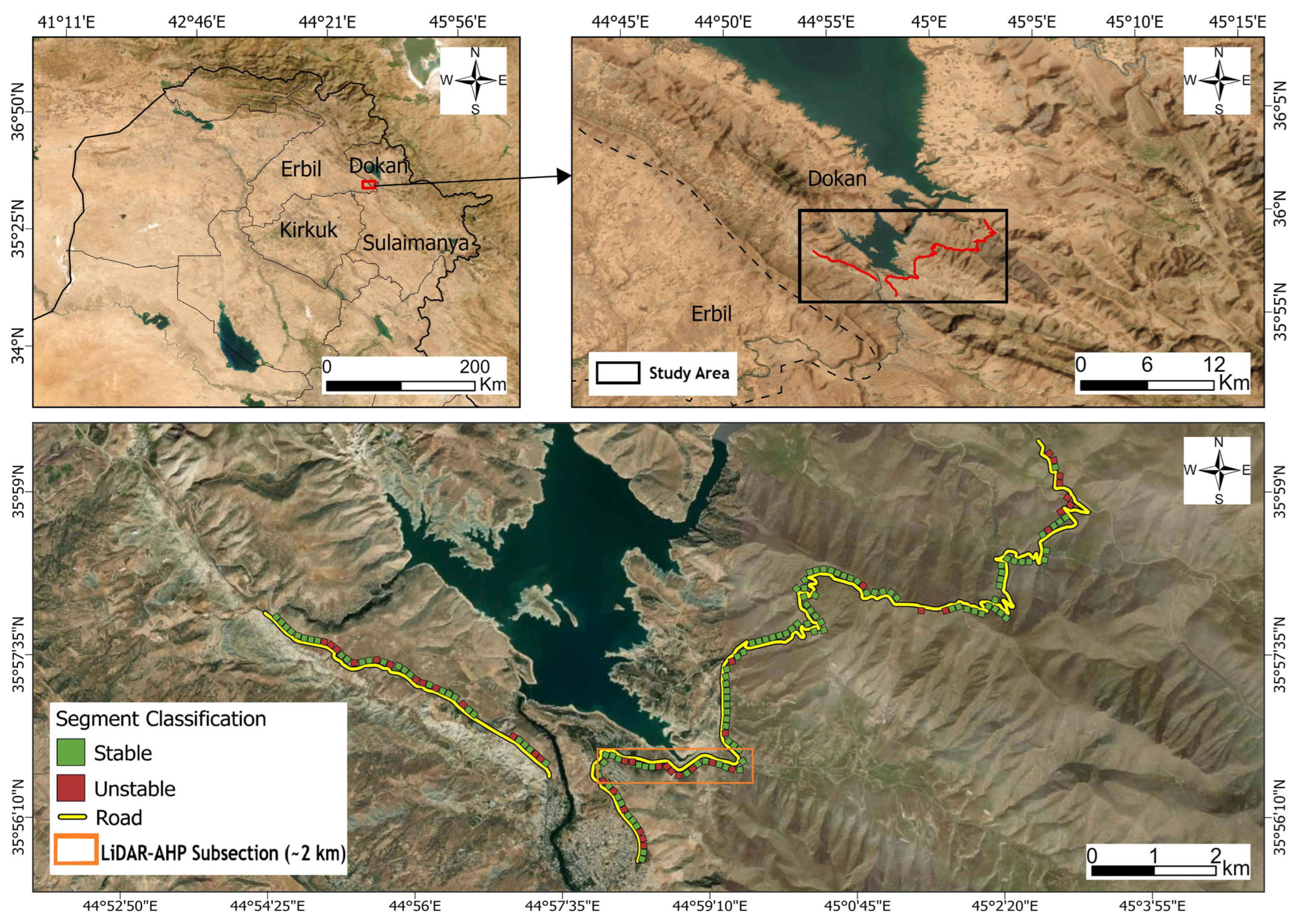
The investigation area is located in As Sulaymaniyah Governorate, northeastern Iraq. The road corridor is approximately 20 km long. It extends from 44°54′10″ E to 45°03′10″ E and from 35°55′50″ N to 35°59′50″ N (WGS84), as shown in Figure 1. Although the geographic extent of the study area is ~14 km × 7 km, the reported road length was measured along its winding alignment through the mountainous terrain, rather than as a straight-line distance. Field surveys indicate that the site consists of rugged limestone terrain. Road cuts increase the likelihood of slope failures. The study site was carefully selected to maintain lithological homogeneity while representing variations in rock units and failure types.
A 2 km section, also depicted in Figure 1, was previously mapped using handheld Simultaneous Localization and Mapping (SLAM) technology (STONEX X120GO SLAM Laser Scanner; STONEX Srl, Paderno Dugnano (MI), Italy) and an AHP-based susceptibility assessment. In this research, the LiDAR dataset was applied as an independent reinforcement layer to compare RF susceptibility assessments within the overlapping section.
The study site was divided into 163 segments (100 × 100 m), including 122 stable and 41 unstable segments. Segments with geomorphological instability scores of 0–2 were classified as stable, whereas those with scores of 3–5 were classified as unstable, as described in Section 2.4. The selected segment size matched the spatial resolution of the conditioning factors used in the analysis. Ten conditioning factors were used in the RF model, whereas the LiDAR–AHP analysis was limited to the overlapping section.

2.2. Overall Methodological Framework

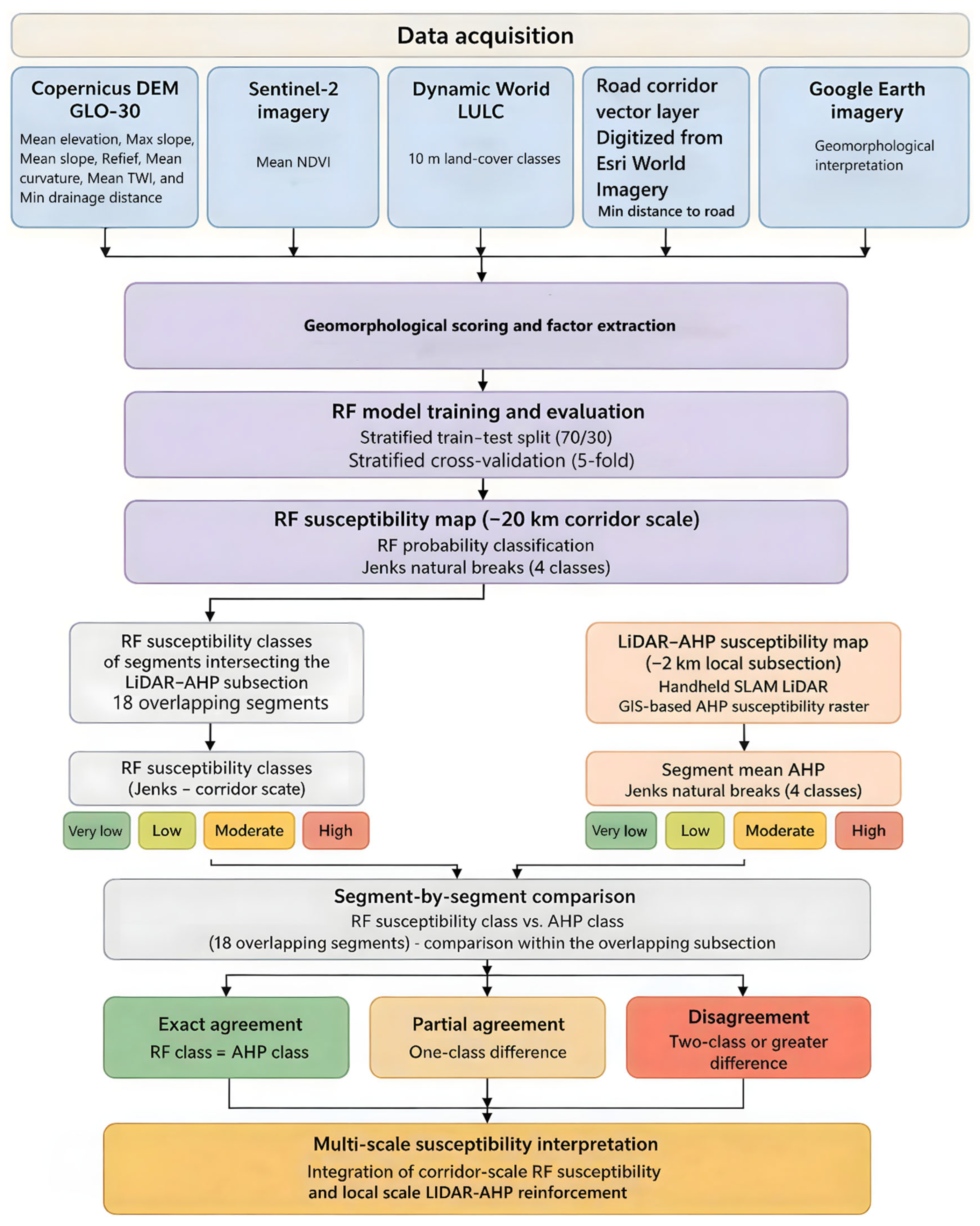
Figure 2 outlines the methodological framework used for corridor-scale landslide susceptibility analysis. The method includes corridor segmentation, geomorphological instability analysis, binarization, conditioning-factor extraction, and RF-based susceptibility modeling.
The methodology comprised corridor segmentation, visual interpretation of instability indicators, geomorphological instability labeling, and conditioning-factor extraction using Google Earth Engine (GEE; Google LLC, Mountain View, CA, USA) and ArcGIS Pro 3.4 (Esri Inc., Redlands, CA, USA). RF-based susceptibility analysis and model-performance evaluation were conducted using Python 3.14.3 (Python Software Foundation, Wilmington, DE, USA) through Visual Studio Code 1.131.0 (Microsoft Corporation, Redmond, WA, USA). An overlapping ~2 km subsection was included for independent multi-scale validation. It was assessed using handheld SLAM LiDAR and a GIS-based AHP susceptibility framework. For each segment, RF and LiDAR–AHP susceptibility classes were compared through ordinal agreement analysis.
The approach was designed for low-inventory scenarios. Its mapping units represent upslope hazard source zones associated with the road corridor rather than regional raster cells [3].

2.3. Corridor Segmentation and Mapping Unit Definition

This corridor is subdivided into 163 segments, each measuring 100 × 100 m, in Google Earth (Google LLC, Mountain View, CA, USA). Segments were outlined in upslope areas near the road corridor, considering the occurrence of geomorphological instability indicators based on visual interpretation. Due to the curved alignment of the road corridor on the mountain slopes, potential hazard source areas can change location between opposite sides of the slope. This depends on topographic conditions and road alignment. This subdivision ensures that the map units reflect the relevant slope area within the terrain, rather than random grids covering the entire area [3,16]. Although each mapping unit has a square geometry (100 × 100 m), it represents a consecutive section of the road corridor and its associated upslope hazard area. Therefore, the term “segment” is used in this study.
The chosen segment size matched the spatial scale of the conditioning factors. It was selected to balance local terrain variability, sufficient data for robust statistical analysis, and a practical evaluation unit for engineering slope assessment. At this scale, each segment contains ~100 raster cells from the 10 m resolution datasets used for factor extraction, providing sufficient representation of topographic and environmental variability within each mapping unit.
The number of segments is a design decision intended to ensure that the analyzed corridor remains within a predominantly fractured carbonate rock setting throughout the project area. If the study area had been extended simply to obtain a larger sample size, this would have resulted in more heterogeneous geological and geomorphological conditions outside of the core area of interest.
The segmentation process did not include areas that did not contribute to the analysis. Hence, the segments used in the analysis were created through topographic segmentation with respect to slope and hazard-source zones. To achieve geometrical consistency, square segments were used in the analysis. The distribution of the segmentation mapping units is presented in Figure 1.

2.4. Instability Indicators, Score Construction, and Binary Labeling

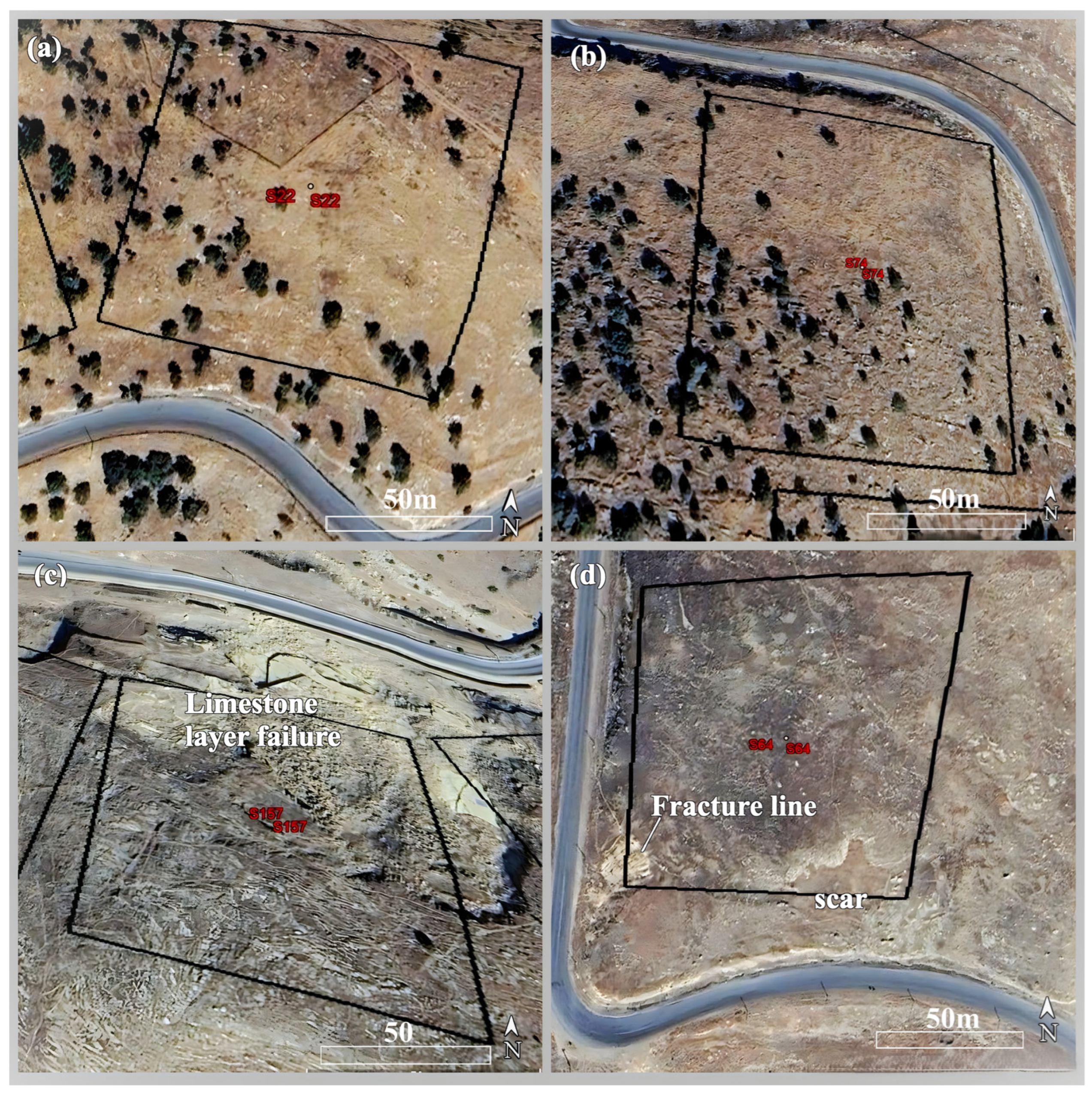
Each segment was visually examined based on five geomorphological categories: scar, debris, fracture, disturbance, and bare rock. ‘Scar’ represents the presence of slope scarp failure; ‘debris’ represents the occurrence of deposition of colluvium. ‘Fracture’ represents discontinuities, whereas ‘disturbance’ represents surface disturbance. ‘Bare rock’ is defined as a rocky outcrop with minimal vegetation cover. These categories were selected considering their suitability from the perspective of field studies and literature reviews [14,17]. The geomorphological interpretation and indicator identification were conducted by the authors through analysis of 2024 Google Earth imagery alongside field observations. It should be noted that Google Earth image analysis has been frequently applied to landslide investigations in areas where no field-based inventories have been made [18]. Stable segments with no noticeable instability characteristics and unstable segments with fractures, bare rocks, and disturbances on the slope are shown in Figure 3a,b and Figure 3c,d, respectively.
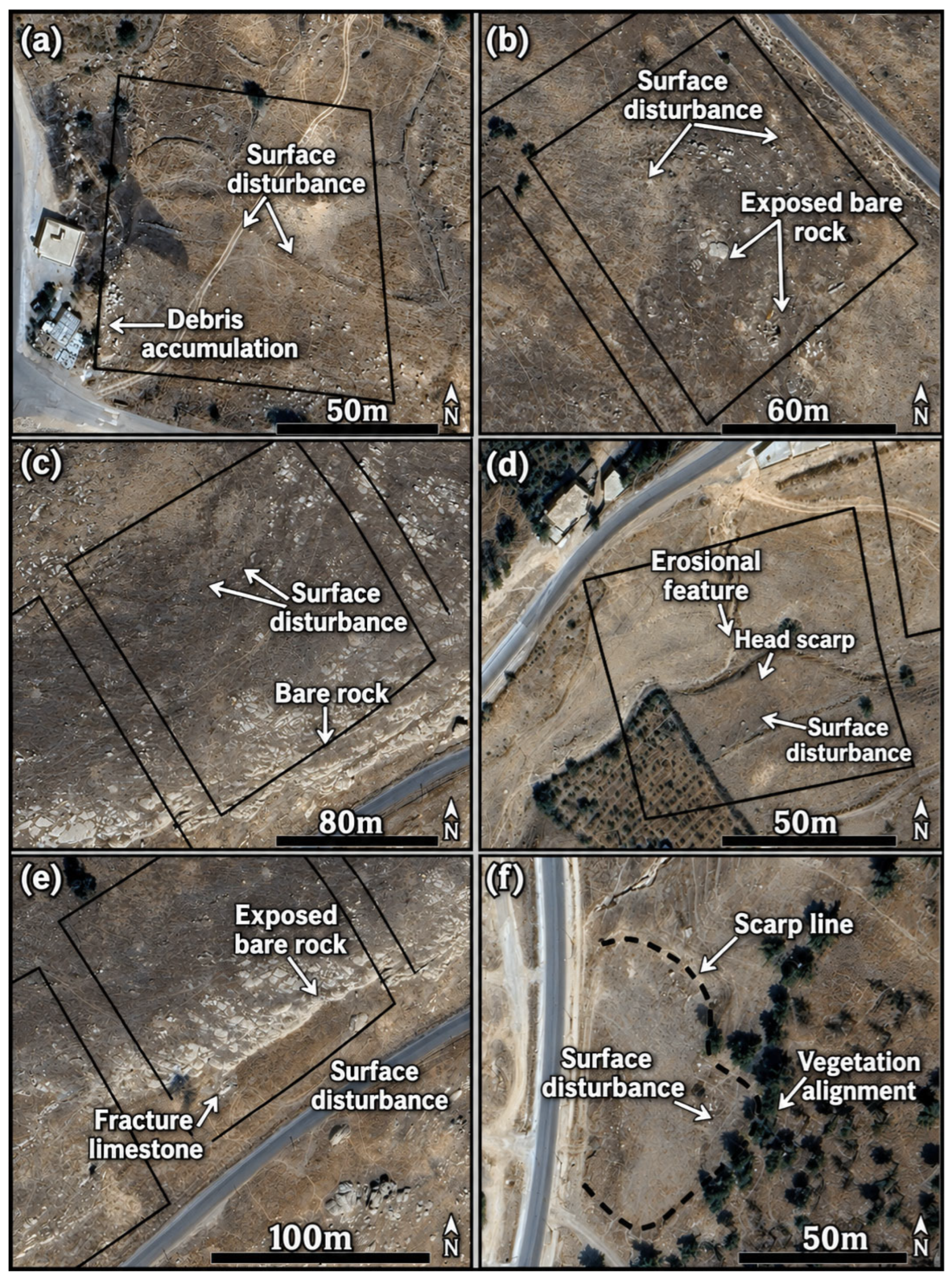
Boundary segments used for the classification system adopted above are shown as representative examples in Figure 4. The segments with a score of 2 are shown in panels (a–c), while segments with a score of 3 are shown in panels (d–f). Each feature received either a presence (1) or absence (0) value, and the instability score for each segment was calculated using Equation (1):
Total Score = Scar + Debris + Fracture + Disturbance + Bare Rock
Those segments with total scores between 0 and 2 were classified as State = 0, whereas those with total scores between 3 and 5 were classified as State = 1. Accordingly, the labeling criterion was defined as Score ≥ 3, indicating that at least three different geomorphological features must co-occur within a single segment. This particular threshold is in line with the idea that slope instability can be more accurately determined using the co-occurrence of multiple geomorphological features rather than a single one. This concept has been widely applied in slope stability assessment [19]. Moreover, slope instability in carbonate terrains is normally determined by the combination of geological, geomorphological, and weathering effects instead of individual factors [20].
This threshold minimizes the likelihood of misclassification by requiring at least three instability indicators within a single segment. However, the interpretation strategy employed a conservative methodology. Features that exhibited partial expression or geomorphological uncertainty were not discarded when there was reasonable evidence of terrain instability. This methodology helped to minimize the probability of overlooking any potentially unstable areas. The final dataset includes 163 segments comprising 122 segments of stability and 41 segments of instability.
In order to validate the geomorphological appropriateness of the chosen threshold, some samples from each boundary type were inspected on Google Earth imagery and during field observations (Figure 4). While segments classified as Score = 2 tend to show weak or inconclusive geomorphological evidence of instability, segments classified as Score = 3 present several co-existing geomorphological signs of slope instability. No scar marks were detected in any segments classified as Score = 2. In contrast, scar marks were present in approximately half of the segments classified as Score = 3. Landslide scarps can be considered as direct evidence of slope instability due to the presence of direct signs of slope movement and material transport [2]. Debris accumulations are widely recognized as key diagnostic indicators in geomorphological landslide inventories [18]. The comparison of boundary classes consequently provides additional support for the adopted threshold (Score ≥ 3), which represents a transition from isolated geomorphological expressions to more evident instability conditions.
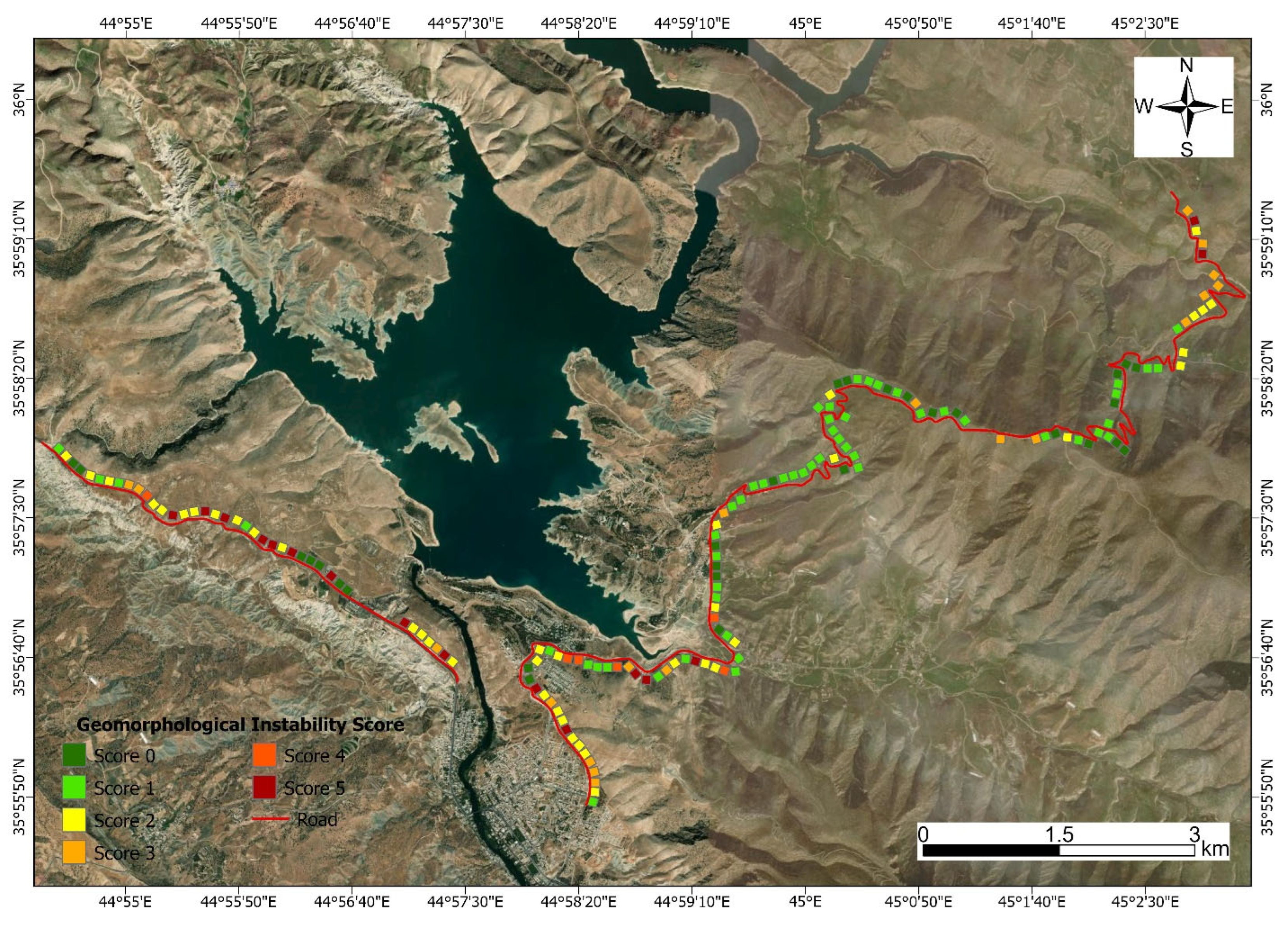
Considering the lack of a landslide inventory database, the chosen scoring method enables an objectively consistent surrogate through observation-based geomorphology. Minor missing data (n = 4) were scored as zero since no observable signs of instability were observed in the interpreted image, thus ensuring consistency in score assignment. The chosen methodology is analogous to heuristic and index-based susceptibility studies undertaken with limited availability of data [1,3]. The spatial distribution of geomorphological instability scores (0–5) is presented in Figure 5 and further discussed in Section 3.

2.5. Conditioning Factors and Segment-Based Extraction

All ten conditioning factors have been considered in the model construction. The above-mentioned parameters were created with the use of GEE and were extracted at the segment scale using zonal statistics and spatial table joins in ArcGIS Pro 3.4. In this way, all predictor variables for all 163 segments have been obtained. Conditioning factors that have been used include those related to terrain, hydrology, vegetation, and land cover, such as the Topographic Wetness Index (TWI) and Land Use/Land Cover (LULC). Conditioning factors, their sources, spatial resolution, and temporal extent used in constructing the RF susceptibility model are outlined in Table 1. The analyzed road corridor is predominantly characterized by exposed fractured carbonate rocks. The selected conditioning factors represent the spatial variability of terrain, hydrological, vegetation, and land-cover characteristics within this environment. GEE is very convenient for carrying out geospatial calculations and extracting environmental factors within a GIS framework [21].
Digital Elevation Model (DEM)-based parameters were resampled to 10 m resolution to be aligned with Sentinel-2 and Dynamic World datasets when extracting segments. In addition, Sentinel-2 imagery acquired from April to October 2024 was used to generate a cloud-filtered median composite to maintain seasonal consistency during factor extraction. As a result, possible time differences between the conditioning factors and geomorphological data could also be avoided. Vegetation was defined using the Normalized Difference Vegetation Index (NDVI) calculated from Sentinel-2 data.
In order to retain consistency in the spatial representation of conditioning factors at the segment scale, the extraction process was conducted to preserve this representation. The mean value of conditioning factors indicates the condition of each segment, while the Maximum slope value is used for identifying critical steepness. This is conducted in such a way that both the overall slope conditions and local steepness can be included in the analysis. Minimum distance to drainage and Minimum distance to road are distance-related variables, and thus the minimum distance representation is used.
Density of lineaments was not included since its reliable extraction from Google Earth imagery at this level could lead to artificial structuring [22]. Other conditioning factors considered at a local scale for the LiDAR-AHP reinforcement approach are discussed separately in the reinforcement methodology section.

2.6. Random Forest Model Development

The data for the last part of the dataset were analyzed using Python 3.14.3 through Visual Studio Code 1.131.0. RF was chosen because of its ability to represent nonlinear functions and handle predictors of different types without the need for stringent distributional assumptions [7]. This makes RF an appropriate choice for datasets related to environmental and geomorphological conditions [6].
RF is resilient to correlated independent variables and does not require complete independence among the conditioning variables. This makes it appropriate for environmental datasets, in which some correlation between independent variables is expected [7,23]. Multicollinearity was assessed using both the Pearson correlation coefficient and the Variance Inflation Factor (VIF). While Pearson correlation was used to detect strongly correlated factor pairs, VIF was applied to evaluate the multivariate collinearity among the conditioning factors. The detailed VIF results are provided in Supplementary Table S1. Three topographic factors (Mean slope, Relief, and Mean elevation) exhibited high VIF values. As a robustness analysis, the RF model was rebuilt after removing the three topographic factors with the highest VIF values (Mean slope, Relief, and Mean elevation). The reduced model showed lower predictive performance across all evaluation metrics than the full model (with ten factors). Therefore, all ten conditioning factors were retained in the final model.
The model was fitted using the ten conditioning variables as predictors and State as the binary target variable. The dataset consisted of 122 stable and 41 unstable segments (roughly a 3:1 ratio). The RF hyperparameters were initially selected based on prior modeling experience and preliminary experimentation. To verify the selected configuration without potential test-set feedback, additional hyperparameter optimization was performed. GridSearchCV from scikit-learn 1.8.0 was applied exclusively to the training subset (70% of the data). Stratified five-fold cross-validation was used with the mean Receiver Operating Characteristic–Area Under the Curve (ROC–AUC) as the optimization criterion, and 180 hyperparameter combinations were evaluated. Based on this analysis, the original RF configuration was retained for the final model. The adopted hyperparameter values were 400 trees, a maximum tree depth of 10, and a minimum leaf size of 2. At each split, the number of features was set to the square root of the total number of features [24].
A threshold value of 0.25 was used rather than the default value of 0.50. It was selected through a threshold sweep analysis (0.05–0.95, step = 0.05) conducted on the independent test subset. The F1-score and Youden’s J statistic (Sensitivity + Specificity − 1) were used as optimization criteria. This threshold was adopted to be more sensitive to unstable segments in classification problems with imbalanced data distributions [25,26]. Both criteria identified 0.25 as the optimal threshold (F1 = 0.581; J = 0.480) (Supplementary Figure S1). In addition, the class threshold was tuned toward the unstable class to address class imbalance. This increased its sensitivity in predicting unstable segments [27,28].
Model validation employed a stratified split of 70% for training and 30% for testing with a fixed random state of 42. Hyperparameter optimization was performed exclusively on the training subset, whereas the independent test subset was reserved solely for the final model evaluation. Model creation and training were performed using the Python programming language in the Visual Studio Code editor.
In order to test whether the model was biased toward vegetation information, an additional robustness analysis was conducted. The Random Forest (RF) model was rebuilt without Mean NDVI while retaining the same training/testing dataset split, RF hyperparameters, and classification threshold. The resulting model was evaluated using the same performance metrics as the full model.

2.7. Model Evaluation

Performance of the model was assessed through Accuracy, Area Under the Receiver Operating Characteristic Curve (AUC), Precision, Recall, F1-score, Specificity, and Cohen’s Kappa. Such measures are broadly used for classification evaluation under imbalanced settings [26,29]. Sensitivity (Recall) was viewed as highly valuable for the current case since it reflected the proportion of unstable segments correctly detected. The Receiver Operating Characteristic (ROC) curve and confusion matrices provided additional insights into discrimination ability and errors made during the classification process [30]. In addition, five-fold stratified cross-validation was conducted during model development to assess model performance on the training dataset [6]. To examine the robustness of the Random Forest (RF) model given the limited number of unstable segments, Monte Carlo cross-validation (MCCV) was performed. The analysis used 500 repeated stratified random 70%/30% train/test splits. During each iteration, the RF model was trained on the training subset and evaluated on the independent test subset. The same RF hyperparameter configuration and classification probability threshold (0.25) were maintained. The resulting performance metrics were summarized using their mean values and corresponding 95% empirical percentile intervals.

2.8. Corridor-Scale Susceptibility Mapping

The RF model trained using the 70% training subset was subsequently applied to all 163 segments to estimate the landslide susceptibility probability of each segment (RF probability). The independent 30% test subset was used exclusively to evaluate model performance before generating the corridor-scale susceptibility map. RF probabilities were divided into four categories according to the Jenks Natural Breaks classification system: Very low, Low, Moderate, and High. This classification supported the visualization of landslide susceptibility and ordinal comparisons between classes generated by the RF and LiDAR–AHP approaches. The Jenks Natural Breaks algorithm classifies continuous RF probability values by minimizing within-class variance and maximizing between-class variance. The corresponding probability boundaries are provided in Supplementary Table S2. The classification of susceptibility into four categories is consistent with previous landslide susceptibility studies that adopted a Very low, Low, Moderate, and High classification framework [31,32]. This method preserves the natural probability structure of RF probabilities and allows for an ordinal comparison of the LiDAR-AHP and RF susceptibility classes.

2.9. LiDAR–AHP Reinforcement and Ordinal Comparison

Previously generated high-resolution susceptibility maps existed for the ~2 km corridor section. This dataset was incorporated as an independent reinforcement layer on a local scale for assessing the susceptibility patterns identified by the RF model at the corridor scale.
The continuous LiDAR-AHP susceptibility raster was reclassified based on the intersecting RF segments (18 segments) using zonal statistics. The mean AHP value was calculated for each RF segment. The segments were then classified into four classes (Very low, Low, Moderate, and High) using the Jenks natural breaks classification technique.
To assess the RF susceptibility classes of intersecting segments, ordinal class-difference analysis was performed against the LiDAR-AHP classes. The analysis considered three categories. Exact agreement represented the same class, partial agreement represented a one-class difference, and total disagreement represented a difference in two or more classes.

3. Results

3.1. Distribution of Geomorphological Instability Scores

Figure 5 shows the spatial distribution of geomorphological instability scores ranging from 0 to 5 across all 163 analyzed segments. Lower scores (0–2) were more often recorded in relatively stable areas along the corridor. Higher scores (3–5) were predominantly observed in areas characterized by steep slopes, road cuts, and exposed limestone outcrops. The clustering of high scores reflects the presence of geomorphological conditions favorable for slope instability development within these areas. Using the proposed labeling approach, only segments having scores greater than or equal to 3 were considered unstable.

3.2. Random Forest Model Performance

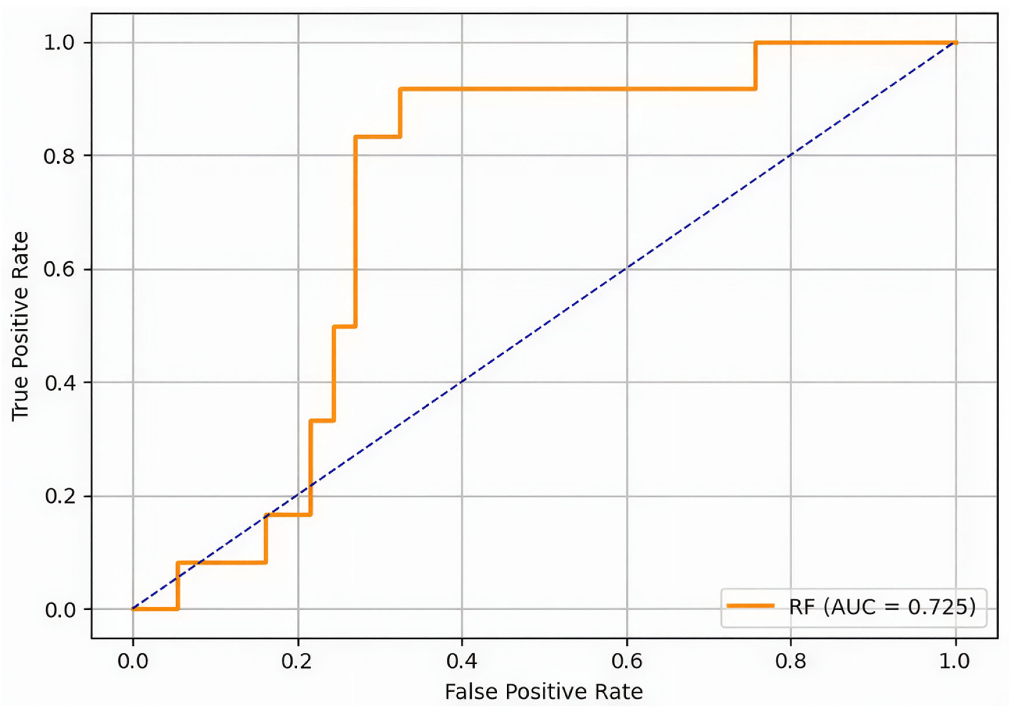
The resulting dataset contained a total of 163 segments consisting of 122 stable and 41 unstable segments. Using five-fold stratified cross-validation, the RF model achieved a mean AUC of 0.783 ± 0.072, indicating acceptable-to-good discrimination ability according to [33]. The cross-validation results suggest that the model performance remained relatively stable across different data partitions, supporting the robustness and generalizability of the RF model for corridor-level landslide susceptibility evaluation. The ROC curve plot shown in Figure 6 lies above the diagonal reference line, demonstrating that the model outperforms random classifiers [30].
For the independent test split, the model achieved an Accuracy of 0.735 and an AUC of 0.725, corresponding to fair discrimination ability according to [33]. Recall was found to be 0.750, which showed that most of the unstable segments were detected. Therefore, the probability threshold was set to 0.25 through the threshold sweep analysis to enhance sensitivity in detecting unstable segments. This selection increased false-positive predictions. The values of Specificity and Cohen’s Kappa coefficient were 0.730 and 0.401, respectively.
Precision (0.474) and the F1-score (0.581) reflect the expected trade-off within a conservative susceptibility-screening framework. The confusion matrix produced 27 true negatives (TN), 9 true positives (TP), 10 false positives (FP), and 3 false negatives (FN), indicating relatively strong sensitivity toward unstable-segment detection. These evaluation metrics are widely applied for evaluating classification performance under imbalanced conditions [26,34].
To determine model stability given the limited number of unstable segments, Monte Carlo cross-validation (MCCV) was performed using 500 randomly generated train/test splits. The Random Forest (RF) model achieved a mean AUC of 0.777 (95% empirical percentile interval: 0.631–0.905) and a mean Precision of 0.418 (0.308–0.542). The mean Cohen’s Kappa was 0.341 (0.129–0.537). The model also maintained a high Recall, with a mean value of 0.849 (95% empirical percentile interval: 0.583–1.000). The complete MCCV results are provided in Supplementary Table S3.
Performance indicators of the predictive models are presented in Table 2, while the ROC curve is provided in Figure 6. Overall, the RF model demonstrated satisfactory predictive performance despite the use of geomorphological proxy classes derived from an inventory-limited dataset.

3.3. Feature Importance

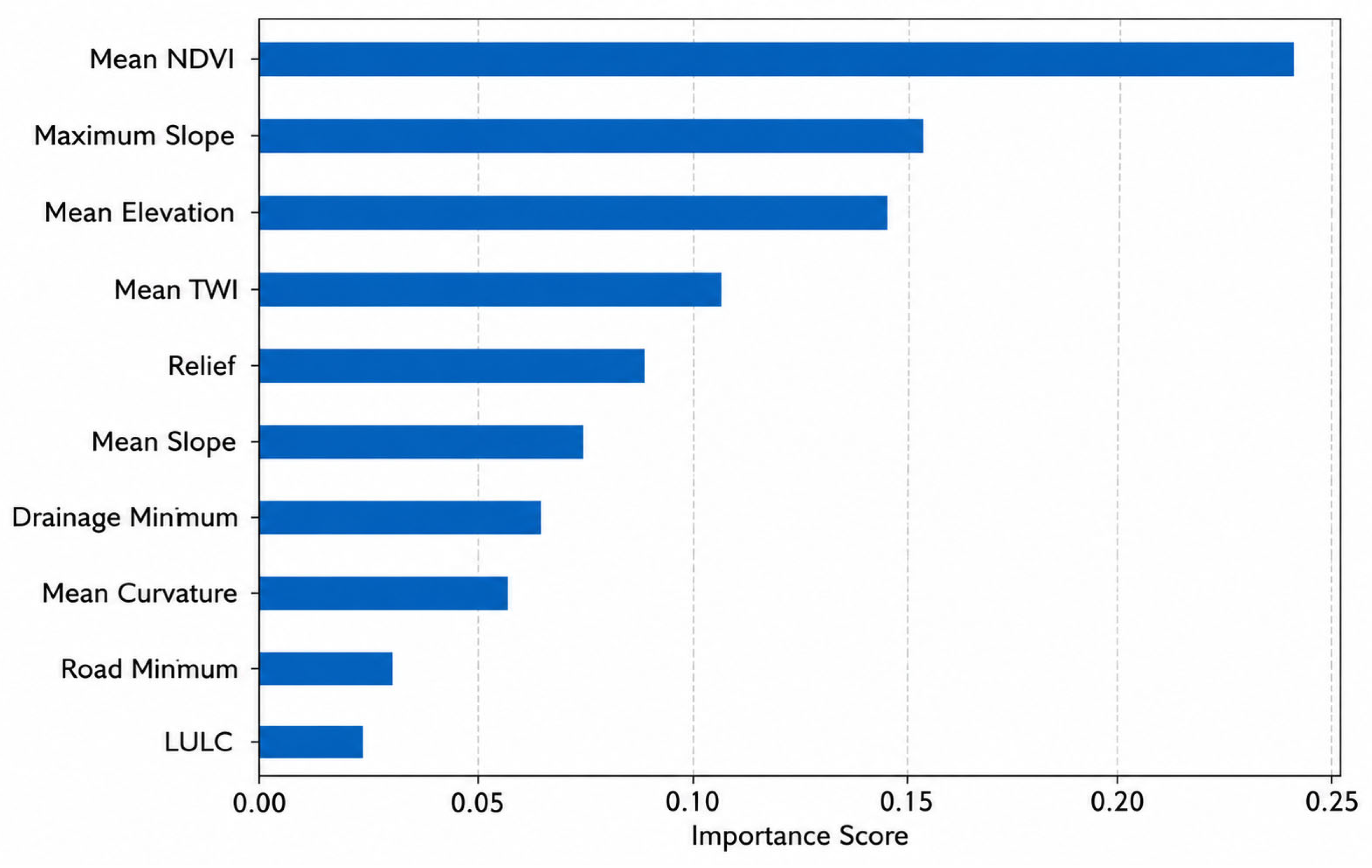
Mean NDVI, Maximum slope, Mean elevation, and Mean TWI were found to be the top predictors, implying that factors like vegetation health, slope steepness, terrain, and moisture heavily influence the model output.
The highest importance among all predictors was found for Mean NDVI, with a value of 0.242. This suggests that NDVI likely acts as a proxy for vegetation cover in terms of surface disturbance and susceptibility. Lower NDVI values have been observed to represent exposed surfaces, fracturing, and disturbed slopes, while higher NDVI values represent stable areas with vegetation growth [35].
To evaluate whether the high importance of Mean NDVI resulted in an over-reliance on vegetation-related information, an additional robustness analysis was performed. The Random Forest (RF) model was rebuilt without Mean NDVI. The ROC–AUC value decreased slightly from 0.725 to 0.716, while the remaining performance metrics showed moderate differences. These results indicate that the RF model maintained comparable predictive performance after excluding Mean NDVI.
The second and third-highest-ranked features were Maximum slope (0.152) and Mean elevation (0.147), demonstrating how local slope steepness and landform positioning play significant roles in determining instability. Importance ratings for Mean TWI (0.107) and Relief (0.089) further indicate the role of moisture storage capacity and elevation differences in slope failure [36].
Less important factors such as Mean slope, Minimum distance to drainage, Mean curvature, Minimum distance to road, and Land Use Land Cover (LULC) contributed to model performance but exhibited comparatively minimal impacts on instability. This could mean that while roads are important, their influence on slope stability cannot be attributed to distance from roads alone. Importance ratings for the features are shown in Table 3 and Figure 7.

3.4. Corridor-Scale Susceptibility Patterns

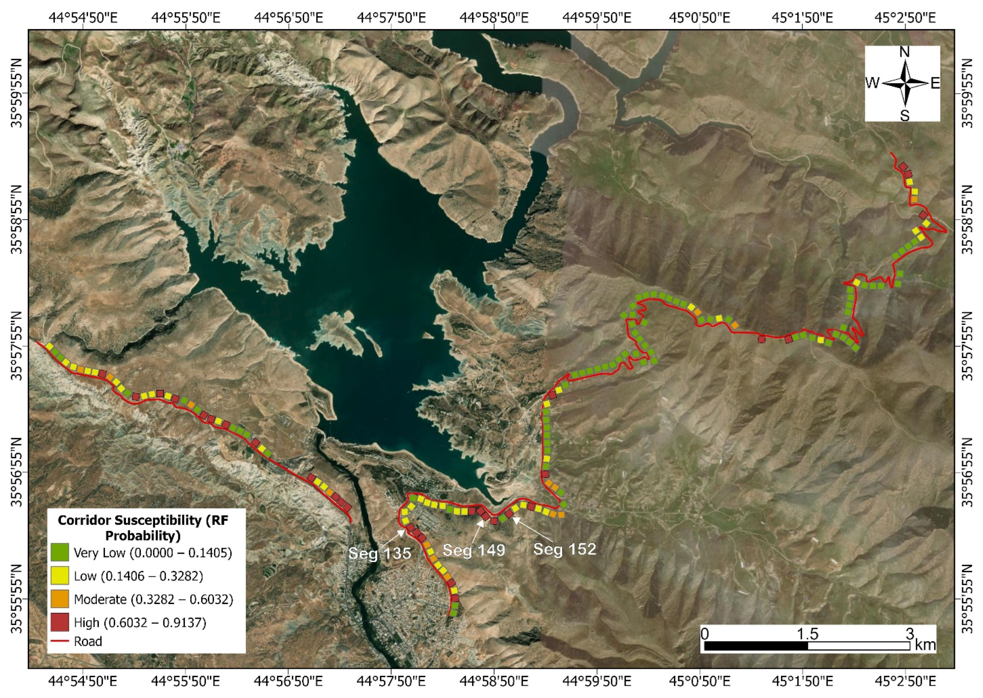
Following the procedure described in Section 2.8, the corridor-scale susceptibility map (Figure 8) reflects RF probabilities generated for all 163 segments. These values differ in scope from the independent test-set metrics reported in Table 2 (Section 3.2). The map shows the spatial pattern of predicted instability along the ~20 km road corridor. The segments were divided into four susceptibility levels using the Jenks Natural Breaks classification: Very low, Low, Moderate, and High. High predicted probabilities of instability were observed for Seg 135 (RF probability = 0.9137), Seg 152 (RF probability = 0.897), and Seg 149 (RF probability = 0.894). Seg 92 and Seg 98 followed these segments. These segments are considered the most susceptible places along the road corridor, hence making them the priority for monitoring and field inspection.
The spatial distribution of susceptibility reveals clusters of moderately and highly susceptible segments in different parts of the road corridor. These susceptibility clusters share similar slope and geological characteristics. They are located in areas with steep slopes and exposed rock surfaces.
However, several other segments with low levels of visual instability also demonstrate high levels of RF probability. For instance, Segs 53 and 163 have an overall score of 0 but RF probabilities above the selected threshold of 0.25. This implies that instability-related conditions may be present in these segments without visible manifestation.
Analysis of RF predictions with respect to geomorphological scores indicated that 20 segments classified as unstable had scores of ≤2. In contrast, only 3 segments with scores of ≥3 were classified as stable. These segments usually had low vegetation cover, steep local slopes, and increased moisture conditions. This suggests that the RF model may identify potentially susceptible segments without clear geomorphological evidence. These segments therefore warrant attention under a risk management approach.

3.5. Reinforcement Within the 2 Km LiDAR Subsection

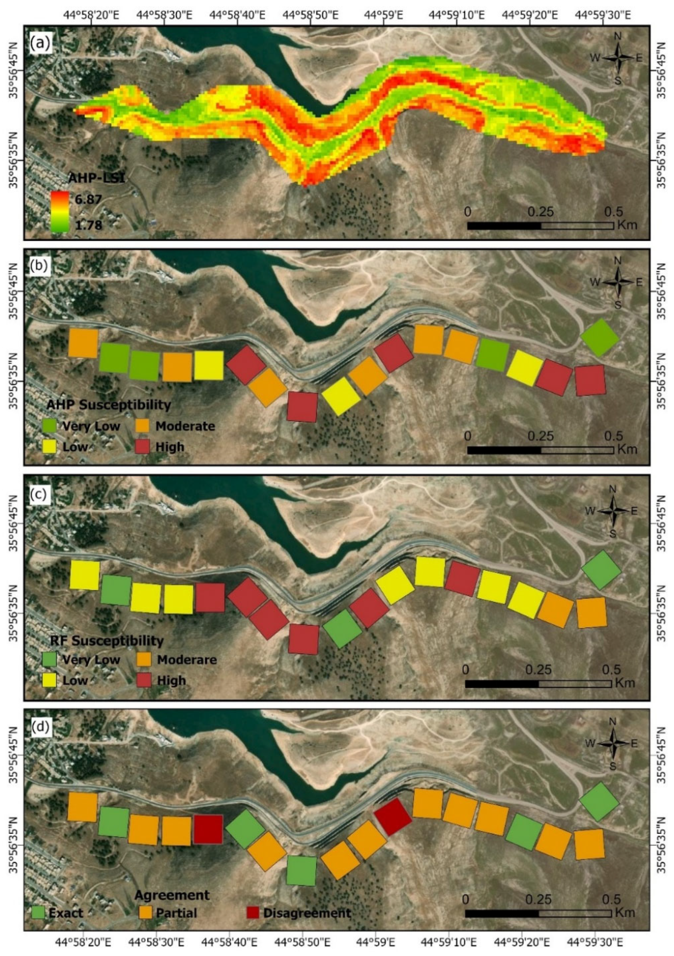
The comparison between the susceptibility models based on RF and LiDAR–AHP methods (Figure 9) demonstrates generally high agreement in the overlapping portion of the study area. This finding is supported by the statistical measures reported in Table 4. The comparison was performed for 18 overlapping segments, taking into consideration four categories of ordinal class ranking (Very low, Low, Moderate, and High).
From the 18 segments, 5 segments (27.8%) show perfect agreement between RF and LiDAR–AHP methods. Another 11 segments (61.1%) exhibit partial agreement with a one-class difference. Agreement between these two models is not observed in only 2 segments (11.1%). Generally, the total percentage of agreement was calculated at 88.9%. Nonetheless, the findings should be interpreted with caution owing to the small sample size (n = 18).
However, it is important to note that the susceptibility classes for the RF and LiDAR–AHP models were independently determined using the Jenks natural breaks method. Consequently, the same ordinal classes (Very low, Low, Moderate, and High) were assessed, but their numerical boundaries differed (Supplementary Table S2). This non-equivalence may have slightly inflated or deflated the observed agreement between the two approaches.
The analysis of agreement shows that the segments having complete and partial agreements were predominantly located in areas characterized by steeper slopes close to roads and exposed fractured limestone bedrock. This confirms that the results obtained in this study were strongly influenced by geomorphological parameters. The majority of the partial agreements were found between adjacent susceptibility classes.
Disagreements are most probably caused by the high sensitivity of the digital topography produced by the LiDAR dataset to local topographic variations. These variations are not represented by the corridor-scale terrain features used by the RF model.
The results suggest that the RF method performs consistently well in landslide susceptibility hazard assessment within the study corridor. In contrast, the LiDAR-AHP technique allows the recognition of finer-scale differences in slope conditions and potential instabilities.

4. Discussion

4.1. Model Performance and Suitability for Corridor-Scale Analysis

RF analysis performed consistently well in evaluating landslide susceptibility at the corridor scale, especially in mountainous road settings characterized by fractured limestone and road-cut slopes [3]. Segment-based mapping increases physical consistency in hazard source delineation by considering upslope areas rather than random raster cells.
Despite the relatively small sample size (n = 163), the controlled geological environment and physically relevant variables provide adequate information to conduct RF screening at the corridor scale. The method achieved an AUC score of 0.725, a Recall of 0.750 (Figure 6; Table 2), and an average cross-validation AUC score of 0.783 ± 0.072. These results demonstrate its effectiveness in identifying unstable segments at the corridor scale under an inadequate landslide inventory. Therefore, the proposed method is viable for susceptibility screening.
Based on the MCCV results, the RF model demonstrated acceptable discrimination across repeated randomly generated data partitions. The mean AUC of 0.777 and the mean Recall of 0.849 were slightly higher than the corresponding values for the independent test set (0.725 and 0.750, respectively). However, the mean Precision of 0.418 and the mean Cohen’s Kappa of 0.341 were slightly lower than the corresponding values of 0.474 and 0.401. This variability is expected because each stratified test subset contained approximately 12 unstable segments. Therefore, the classification of only a few segments could noticeably affect threshold-dependent metrics, including Precision, F1-score, Specificity, and Cohen’s Kappa. The higher Recall and lower Precision are consistent with the selected probability threshold of 0.25, which favored the detection of unstable segments.
The adopted probability threshold of 0.25 further increased the detection rate of instability. In infrastructure risk assessment, missed instabilities might directly affect road stability and thus represent additional risk [37,38]. High probabilities were calculated in some areas with low visual instability scores. This demonstrates that the RF approach considers terrain features related to instability beyond those included in the labeling process. Overall, the achieved results indicate that RF presents a physically interpretable approach to susceptibility screening along the studied corridor.

4.2. Interpretation of Dominant Conditioning Factors and Susceptibility Patterns

According to the feature importance analysis shown in Figure 7 and Table 3, four groups are the predominant variables affecting model predictions. These are vegetation condition (Mean NDVI), slope geometry (Maximum slope), terrain position (Mean elevation), and moisture-related factors (Mean TWI).
Given the high significance of the Mean NDVI factor, vegetation condition acts as an indirect proxy for disturbance and slope instability. Low values of NDVI are linked to the exposure of rock surfaces, disturbed landforms, and low vegetation coverage, while high values reflect relatively stable slope landforms [39]. This conclusion correlates well with the field observations and unstable slope segments illustrated in Figure 3.
The robustness analysis further showed that excluding Mean NDVI resulted in only a slight reduction in model performance. This suggests that Mean NDVI was the most influential predictor, but the RF model did not rely solely on vegetation-related information. The remaining topographic and hydrological conditioning factors continued to provide substantial predictive capability.
To further evaluate the role of vegetation condition, Mean NDVI distributions were compared between stable and unstable segments (Supplementary Figure S2). Stable segments exhibited higher Mean NDVI values (mean = 0.187 ± 0.060; range = 0.092–0.342) than unstable segments (mean = 0.143 ± 0.035; range = 0.100–0.295). The difference between the two groups was statistically significant (Mann–Whitney U test, p < 0.001) [40], providing empirical support for the high ranking of Mean NDVI in the RF feature-importance analysis.
Maximum slope had a higher significance level than Mean slope. This indicates that the local slope gradient had a greater effect on triggering instability than the mean slope gradient at the segment scale. The parameters Mean TWI and Relief highlight the impact of moisture accumulation and topography on instability [39].
As depicted in Figure 8, the susceptibility maps at the corridor scale reveal a noticeable clustering of moderate to high susceptibility classes in the steeper and more topographically complex parts of the corridor. Some segments that lack geomorphological expression show higher probabilities as well, indicating that these segments might be prone to instability without showing geomorphological evidence.
These results are consistent with previous landslide susceptibility studies conducted in northeastern Iraq and the Kurdistan Region. These studies highlighted the roles of slope morphology, lithology, and geological structures in the development of instability patterns [8,9,41].

4.3. Reliability, Reinforcement, and Multi-Scale Consistency

The geomorphology labeling scheme adopted reflects an example of a proxy-based classification methodology carried out under constrained inventory circumstances. While interpretative uncertainty may be inevitable to some extent, the application of standard binary measures and scores enhances reliability across all segments [5].
This further enhances the credibility of the classification approach through the LiDAR-AHP validation analysis (Figure 9; Table 4). It provides an independent basis for comparison of both approaches at high resolution. The high degree of exact and partial agreement found between the two methods demonstrates strong spatial agreement within the common subsection.
Given the few disagreements (11.1%), the RF model exhibits overall consistency in identifying corridor susceptibility. However, high-resolution LiDAR data are more sensitive to topographical and structural nuances within local microtopography than corridor-scale RF predictors. This may explain the few areas of disagreement.
This is expected because corridor-level RF predictors capture segment-level conditions. In contrast, LiDAR-based Susceptibility surfaces capture localized slope and topographical variations within individual segments. This indicates that both RF and LiDAR-AHP models generate complementary spatial perspectives at the corridor and local scales.

4.4. Limitations and Future Research

Several limitations must be accounted for while analyzing the results. First, the dataset under analysis is not large (163 segments). The labeling scheme used is geomorphologically based and does not include a full inventory of landslides. Accordingly, the labeling scheme involves uncertainty due to the geomorphological interpretation of remote sensing imagery. This uncertainty is particularly relevant when unstable morphologies occur only partially. Finally, the analysis is confined to a fractured limestone zone, and thus its application might not be universal in geological terms.
Although field observations indicated that the exposed road-cut slopes are predominantly characterized by fractured carbonate rocks, local variations in rock composition, bedding, and structural fracturing may still exist. These variations were not explicitly quantified. Therefore, the applicability of the proposed framework to areas with greater geological heterogeneity should be evaluated carefully.
This was an intentional choice in the methodology to exclude lineament density. Even if the corridor itself is structurally controlled, there may be a potential for interpretation error when extracting structural lineaments from imagery at this scale [22]. Therefore, physical and hydrological predictors were emphasized over unreliable structural ones.
The LiDAR–AHP reinforcement method is also constrained by its application to an overlapping section of about 2 km and is not applied throughout the corridor. Further studies on this subject should extend the high-resolution LiDAR data range, use multi-temporal data, and assess other environmental controls, such as rainfall and seismicity. Testing the applicability of the proposed framework on other mountainous corridors would also be helpful.

5. Conclusions

In summary, the results from this research show that a segment-based Random Forest approach is an efficient means of conducting landslide susceptibility assessment at the corridor scale. The approach is intended for narrow road corridors within mountainous regions with limited inventory data. A combination of geomorphological indicators and physical variables ensures both interpretability and accuracy.
The RF model demonstrated fair discrimination ability and useful screening capability, achieving a mean five-fold stratified cross-validation AUC of 0.783 ± 0.072 and an independent test AUC of 0.725. The model was also able to detect potentially unstable areas while reducing false negatives. Feature importance analysis revealed the controlling factors of slope instability, which include vegetation conditions (Mean NDVI), slope characteristics (Maximum slope), topographic position (Mean elevation), and moisture processes (Mean TWI).
Inclusion of a high-resolution LiDAR-AHP dataset as a reinforcement layer can be viewed as a significant achievement of the research. It allowed the development of a multi-scale reinforcement strategy for analyzing RF susceptibility patterns at the corridor scale.
Analysis of the reinforcement demonstrated a high degree of spatial correspondence between RF and LiDAR-AHP classifications, which is characterized by a large proportion of areas with exact and partial agreement. Small discrepancy values also provide evidence of the physical consistency of the susceptibility patterns modeled using RF and LiDAR-AHP data.
The suggested framework has been designed with consideration of its practical utility for hazard analysis and infrastructure hazard management. This design ensures the physical interpretability and applicability of the framework for landslide susceptibility mapping along the corridor.

Supplementary Materials

The following supporting information can be downloaded at: https://www.mdpi.com/article/10.3390/geohazards7030093/s1, Table S1: Variance Inflation Factor (VIF) values for the ten conditioning factors used in the RF model; Table S2: Jenks natural break boundaries used for RF probability and LiDAR–AHP susceptibility classifications in the comparison of the 18 overlapping segments within the 2 km LiDAR subsection; Table S3: Summary statistics of the Monte Carlo cross-validation (MCCV) analysis (500 repeated stratified train/test splits), showing the mean, standard deviation (SD), and 95% empirical percentile interval for each performance metric; Figure S1: Threshold sweep analysis showing the variation in Sensitivity, Specificity, Precision, F1-score, and Youden’s J statistic across candidate probability thresholds (0.05–0.95, step = 0.05) evaluated on the independent test dataset. The selected threshold (0.25) corresponds to the highest F1-score and Youden’s J statistic among the evaluated thresholds; Figure S2: Box plot comparing Mean NDVI distributions between stable (n = 122) and unstable (n = 41) segments. Boxes represent the interquartile range, the central line indicates the me-dian, whiskers denote data dispersion, and circles represent outliers.

Author Contributions

Conceptualization, R.S.M.A.; methodology, R.S.M.A., Q.A.M.A. and A.A.O.; field investigation, R.S.M.A.; data curation, R.S.M.A.; geospatial analysis, R.S.M.A.; susceptibility modeling, R.S.M.A.; formal analysis, R.S.M.A.; visualization, R.S.M.A.; interpretation of results, R.S.M.A.; writing—original draft preparation, R.S.M.A.; writing—review and editing, Q.A.M.A. and A.A.O.; supervision, Q.A.M.A. and A.A.O. All authors have read and agreed to the published version of the manuscript.

Funding

This research received no external funding.

Data Availability Statement

The raw data supporting the conclusions of this article will be made available by the authors on request.

Conflicts of Interest

The authors declare no conflicts of interest.

References

  1. Guzzetti, F.; Carrara, A.; Cardinali, M.; Reichenbach, P. Landslide hazard evaluation: A review of current techniques and their application in a multi-scale study, Central Italy. Geomorphology 1999, 31, 181–216. [Google Scholar] [CrossRef] [Scilit]
  2. Hungr, O.; Leroueil, S.; Picarelli, L. The Varnes classification of landslide types, an update. Landslides 2014, 11, 167–194. [Google Scholar] [CrossRef] [Scilit]
  3. Reichenbach, P.; Rossi, M.; Malamud, B.D.; Mihir, M.; Guzzetti, F. A review of statistically-based landslide susceptibility models. Earth. Sci. Rev. 2018, 180, 60–91. [Google Scholar] [CrossRef] [Scilit]
  4. Velazco, S.; Rodríguez, Á.; Riascos, M.; Nieto, F.; Granados, D. Evaluation of Landslide Risk Using the WoE and IV Methods: A Case Study in the Zipaquirá–Pacho Road Corridor. GeoHazards 2025, 6, 27. [Google Scholar] [CrossRef] [Scilit]
  5. Pham, B.; Shirzadi, A.; Shahabi, H.; Omidvar, E.; Singh, S.K.; Sahana, M.; Talebpour Asl, D.; Bin Ahmad, B.; Kim Quoc, N.; Lee, S. Landslide susceptibility assessment by novel hybrid machine learning algorithms. Sustainability 2019, 11, 4386. [Google Scholar] [CrossRef] [Scilit]
  6. Chen, X.; Chen, W. GIS-based landslide susceptibility assessment using optimized hybrid machine learning methods. CATENA 2021, 196, 104833. [Google Scholar] [CrossRef] [Scilit]
  7. Breiman, L. Random Forests. Mach. Learn. 2001, 45, 5–32. [Google Scholar] [CrossRef] [Scilit]
  8. Othman, A.A.; Gloaguen, R. Automatic extraction and size distribution of landslides in Kurdistan Region, NE Iraq. Remote Sens. 2013, 5, 2389–2410. [Google Scholar] [CrossRef] [Scilit]
  9. Othman, A.A.; Gloaguen, R.; Andreani, L.; Rahnama, M. Landslide susceptibility mapping in Mawat area, Kurdistan Region, NE Iraq: A comparison of different statistical models. Nat. Hazards Earth Syst. Sci. Discuss. 2015, 3, 1789–1833. [Google Scholar]
  10. Othman, A.A.; Al-Jaff, A.U.; Al-Manmi, D.A.; Al-Maamar, A.F. Landslide susceptibility mapping using remote sensing and GIS application: A case study in Qala Diza and surrounding area, Kurdistan Region, NE Iraq. Iraqi Bull. Geol. Min. 2018, 14, 65–90. [Google Scholar]
  11. Qader, W.M.; Noori, A.M.; Omer, F.M.; Al Nuaimy, Q.A.M.; Saed, F.G. Soil erosion susceptibility mapping by analyzing morphometric parameters using ALOS PALSAR DEM and GIS techniques for Rawanduz River Basins in Iraq. In Selected Studies in Geomorphology, Sedimentology, and Geochemistry: Proceedings of the 3rd Conference of the Arabian Journal of Geosciences (CAJG-3); Lucci, F., Doronzo, D.M., Knight, J., et al., Eds.; Springer: Cham, Switzerland, 2023; pp. 89–93. [Google Scholar] [CrossRef] [Scilit]
  12. Bashir, B.; Alsalman, A.; Othman, A.A.; Obaid, A.K.; Bashir, H. New approach to selecting civil defense centers in Al-Riyadh City (KSA) based on multi-criteria decision analysis and GIS. Land 2021, 10, 1108. [Google Scholar] [CrossRef] [Scilit]
  13. Lombardo, L.; Mai, P.M. Presenting logistic regression-based landslide susceptibility results. Eng. Geol. 2018, 244, 14–24. [Google Scholar] [CrossRef] [Scilit]
  14. Jaboyedoff, M.; Oppikofer, T.; Abellán, A.; Derron, M.-H.; Loye, A.; Metzger, R.; Pedrazzini, A. Use of LiDAR in landslide investigations: A review. Nat. Hazards 2012, 61, 5–28. [Google Scholar] [CrossRef] [Scilit]
  15. Tarolli, P. High-resolution topography for understanding Earth surface processes: Opportunities and challenges. Geomorphology 2014, 216, 295–312. [Google Scholar] [CrossRef] [Scilit]
  16. Fu, X.; Liu, Y.; Zhu, Q.; Ge, D.; Li, Y.; Zeng, H. Reliable assessment approach of landslide susceptibility in broad areas based on optimal slope units and negative samples involving priori knowledge. Int. J. Digit. Earth 2022, 15, 2495–2510. [Google Scholar] [CrossRef] [Scilit]
  17. Abellán, A.; Oppikofer, T.; Jaboyedoff, M.; Rosser, N.; Lim, M.; Lato, M. Terrestrial laser scanning of rock slope instabilities. Earth Surf. Process. Landf. 2014, 39, 80–97. [Google Scholar] [CrossRef] [Scilit]
  18. Guzzetti, F.; Mondini, A.C.; Cardinali, M.; Fiorucci, F.; Santangelo, M.; Chang, K.-T. Landslide inventory maps: New tools for an old problem. Earth. Sci. Rev. 2012, 112, 42–66. [Google Scholar] [CrossRef] [Scilit]
  19. Raghuvanshi, T.K.; Ibrahim, J.; Ayalew, D. Slope stability susceptibility evaluation parameter (SSEP) rating scheme—An approach for landslide hazard zonation. J. Afr. Earth Sci. 2014, 99, 595–612. [Google Scholar] [CrossRef] [Scilit]
  20. Azarafza, M.; Hajialilue Bonab, M.; Derakhshani, R. A novel empirical classification method for weak rock slope stability analysis. Sci. Rep. 2022, 12, 14744. [Google Scholar] [CrossRef] [Scilit] [PubMed]
  21. Gorelick, N.; Hancher, M.; Dixon, M.; Ilyushchenko, S.; Thau, D.; Moore, R. Google Earth Engine: Planetary-scale geospatial analysis for everyone. Remote Sens. Environ. 2017, 202, 18–27. [Google Scholar] [CrossRef] [Scilit]
  22. Ahmadi, H.; Pekkan, E. Fault-based geological lineaments extraction using remote sensing and GIS—A review. Geosciences 2021, 11, 183. [Google Scholar] [CrossRef] [Scilit]
  23. Kuhn, M.; Johnson, K. Applied Predictive Modeling; Springer: New York, NY, USA, 2013; Volume 26. [Google Scholar]
  24. Probst, P.; Wright, M.N.; Boulesteix, A. Hyperparameters and tuning strategies for random forest. Wiley Interdiscip. Rev. Data Min. Knowl. Discov. 2019, 9, e1301. [Google Scholar] [CrossRef] [Scilit]
  25. Fernández, A.; García, S.; Galar, M.; Prati, R.C.; Krawczyk, B.; Herrera, F. Learning from Imbalanced Data Sets; Springer: Cham, Switzerland, 2018; Volume 10. [Google Scholar]
  26. Chicco, D.; Jurman, G. The Matthews correlation coefficient (MCC) should replace the ROC AUC as the standard metric for assessing binary classification. BioData Min. 2023, 16, 4. [Google Scholar] [CrossRef] [Scilit] [PubMed]
  27. Ghosh, K.; Bellinger, C.; Corizzo, R.; Branco, P.; Krawczyk, B.; Japkowicz, N. The class imbalance problem in deep learning. Mach. Learn. 2024, 113, 4845–4901. [Google Scholar] [CrossRef] [Scilit]
  28. Shehab, S.A.; Darwish, A.; Hassanien, A.E. Water quality classification model with small features and class imbalance based on fuzzy rough sets. Environ. Dev. Sustain. 2025, 27, 1401–1419. [Google Scholar] [CrossRef] [Scilit]
  29. Sokolova, M.; Lapalme, G. A systematic analysis of performance measures for classification tasks. Inf. Process. Manag. 2009, 45, 427–437. [Google Scholar] [CrossRef] [Scilit]
  30. Fawcett, T. ROC graphs with instance-varying costs. Pattern Recognit. Lett. 2006, 27, 882–891. [Google Scholar] [CrossRef] [Scilit]
  31. Li, M.; Wang, H.; Chen, J.; Zheng, K. Assessing landslide susceptibility based on the random forest model and multi-source heterogeneous data. Ecol. Indic. 2024, 158, 111600. [Google Scholar] [CrossRef] [Scilit]
  32. Lv, M.; Li, K.; Cai, J.; Mao, J.; Gao, J.; Xu, H. Evaluation of landslide susceptibility based on SMOTE-Tomek sampling and machine learning algorithm. PLoS ONE 2025, 20, e0323487. [Google Scholar] [CrossRef] [Scilit] [PubMed]
  33. Swets, J.A. Measuring the accuracy of diagnostic systems. Science 1988, 240, 1285–1293. [Google Scholar] [CrossRef] [Scilit]
  34. Agboola, G.; Beni, L.H.; Elbayoumi, T.; Thompson, G. Optimizing landslide susceptibility mapping using machine learning and geospatial techniques. Ecol. Inform. 2024, 81, 102583. [Google Scholar] [CrossRef] [Scilit]
  35. Niraj, K.C.; Singh, A.; Shukla, D.P. Effect of the normalized difference vegetation index (NDVI) on GIS-enabled bivariate and multivariate statistical models for landslide susceptibility mapping. J. Indian Soc. Remote Sens. 2023, 51, 1739–1756. [Google Scholar] [CrossRef] [Scilit]
  36. Chakrabortty, R.; Pal, S.C.; Roy, P.; Saha, A.; Chowdhuri, I. Novel ensemble approach for landslide susceptibility index assessment in a mountainous environment of India. Geocarto Int. 2022, 37, 13311–13336. [Google Scholar] [CrossRef] [Scilit]
  37. Gupta, K.; Yunus, A.P.; Siddique, T.; Ahamad, A. Landslide susceptibility along National Highway-7 in the Himalayas using random forest-based machine learning tool. J. Earth Syst. Sci. 2025, 134, 74. [Google Scholar] [CrossRef] [Scilit]
  38. Wang, B.; Zuo, Q.; Deng, M.; Yi, Q.; Ruan, D.; Liang, Z. Study on the deformation mechanism of chair-like bedding rock landslides under the coupling effect of geological and hydrological factors. Eng. Geol. 2025, 344, 107832. [Google Scholar] [CrossRef] [Scilit]
  39. Zhao, S.; Dai, F.; Deng, J.; Wen, H.; Li, H.; Chen, F. Insights into landslide development and susceptibility in extremely complex alpine geoenvironments along the Western Sichuan–Tibet Engineering Corridor, China. CATENA 2023, 227, 107105. [Google Scholar] [CrossRef] [Scilit]
  40. Mann, H.B.; Whitney, D.R. On a test of whether one of two random variables is stochastically larger than the other. Ann. Math. Stat. 1947, 18, 50–60. [Google Scholar] [CrossRef] [Scilit]
  41. Othman, A.A.; Gloaguen, R.; Andreani, L.; Rahnama, M. Improving landslide susceptibility mapping using morphometric features in the Mawat area, Kurdistan Region, NE Iraq: Comparison of different statistical models. Geomorphology 2018, 319, 147–160. [Google Scholar] [CrossRef] [Scilit]
Figure 1. Location of the study area in northeastern Iraq, showing the ~20 km road corridor with the 163 segments classified as stable (n = 122) and unstable (n = 41), and the overlapping LiDAR–AHP subsection (~2 km). Basemap source: Esri World Imagery (accessed in 2026) and administrative boundaries from GADM.
Geohazards 07 00093 g001
Figure 2. Overall methodological workflow.
Geohazards 07 00093 g002
Figure 3. Representative examples of stable and unstable segments identified from Google Earth imagery (2024) along the study corridor in northeastern Iraq. Panels (a,b) represent stable segments with limited geomorphological evidence of instability, while panels (c,d) represent unstable segments characterized by geomorphological features such as limestone slope failures, fracture zones, and scarps. The center coordinates of the segments in panels (ad) are 35.968647° N, 45.015405° E; 35.972660° N, 45.037990° E; 35.943229° N, 44.988864° E; and 35.984458° N, 45.048412° E, respectively.
Geohazards 07 00093 g003
Figure 4. Representative examples of segments located at the classification boundary of the adopted binary labeling scheme. Panels (ac) show segments assigned a score of 2, whereas panels (df) show segments assigned a score of 3. The center coordinates of panels (af) are 35.974381° N, 45.045657° E; 35.979441° N, 45.049547° E; 35.978186° N, 45.047558° E; 35.958837° N, 44.989783° E; 35.977784° N, 45.046554° E; and 35.931862° N, 44.974132° E, respectively, in the WGS 84 geographic coordinate system.
Geohazards 07 00093 g004
Figure 5. Spatial distribution of geomorphological instability scores (0–5) across the 163 segments of the study corridor, using a graduated color scheme from dark green (Score 0, most stable) through light green, yellow, orange, and orange-red to dark red (Score 5, most unstable). Basemap source: Esri World Imagery (accessed in 2026).
Geohazards 07 00093 g005
Figure 6. ROC curve of the RF model (AUC = 0.725).
Geohazards 07 00093 g006
Figure 7. RF feature importance showing the relative contribution of conditioning factors to landslide susceptibility classification.
Geohazards 07 00093 g007
Figure 8. Corridor-scale RF susceptibility map showing 163 segments classified into four Jenks-based susceptibility classes (green = Very Low, yellow = Low, orange = Moderate, red = High). Class value ranges are provided in the map legend.
Geohazards 07 00093 g008
Figure 9. LiDAR–AHP reinforcement analysis within the overlapping ~2 km subsection: (a) LiDAR–AHP susceptibility raster; (b) LiDAR–AHP susceptibility classes; (c) RF susceptibility classes; and (d) agreement map. Class colors and value ranges are provided in the legend of each panel.
Geohazards 07 00093 g009
Table 1. Conditioning factors, source datasets, spatial resolution, and acquisition period used in the RF susceptibility model.
Conditioning FactorSource DatasetSpatial ResolutionAcquisition Year/Access Year
Mean elevationCopernicus DEM GLO-30Resampled to 10 mAccessed in 2026
ReliefCopernicus DEM GLO-30Resampled to 10 mAccessed in 2026
Mean slopeCopernicus DEM GLO-30Resampled to 10 mAccessed in 2026
Maximum slopeCopernicus DEM GLO-30Resampled to 10 mAccessed in 2026
Minimum distance to drainageDEM-derived drainage networkResampled to 10 mAccessed in 2026
Mean curvatureCopernicus DEM GLO-30Resampled to 10 mAccessed in 2026
Mean TWICopernicus DEM GLO-30Resampled to 10 mAccessed in 2026
Mean NDVISentinel-2 10 mApril–October 2024 (median composite)
LULCDynamic World V1 land-cover dataset10 mApril–October 2024 (median composite)
Minimum distance to roadDigitized GIS road corridor layerAccessed in 2026
Table 2. Performance metrics of the RF model under stratified 70/30 train–test validation.
MetricValue
Accuracy0.735
AUC 0.725
Cohen’s Kappa0.401
Recall (Unstable class)0.750
Specificity (Stable)0.730
Precision (Unstable)0.474
F1-score (Unstable)0.581
Probability threshold0.250
Table 3. Feature importance ranking derived from the RF for landslide susceptibility classification.
RankFeatureImportance Score
1Mean NDVI0.242
2Maximum slope0.152
3Mean elevation0.147
4Mean TWI0.107
5Relief0.089
6Mean slope0.075
7Minimum distance to drainage0.067
8Mean curvature0.060
9Minimum distance to road0.034
10LULC0.026
Table 4. Agreement statistics between Random Forest and LiDAR–AHP classifications within the overlapping ~2 km subsection.
Agreement CategoryClass DifferenceNumber of SegmentsPercentage (%)
Exact agreement0527.8
Partial agreement11161.1
Disagreement≥2211.1
Exact + Partial agreement *≤11688.9
* Exact and partial agreement together represent segments differing by no more than one susceptibility class.
Disclaimer/Publisher’s Note: The statements, opinions and data contained in all publications are solely those of the individual author(s) and contributor(s) and not of MDPI and/or the editor(s). MDPI and/or the editor(s) disclaim responsibility for any injury to people or property resulting from any ideas, methods, instructions or products referred to in the content.