Article

Korean Peninsula—Updated Sea-Level Rise Assessment


1
US Coastal Education and Research Foundation, Lawrence, KS 66044, USA
2
Marine Disaster Research Center, Korea Institute of Ocean Science and Technology, Busan 49111, Republic of Korea
*
Author to whom correspondence should be addressed.
GeoHazards 2026, 7(2), 51; https://doi.org/10.3390/geohazards7020051
Submission received: 17 March 2026 / Revised: 20 April 2026 / Accepted: 27 April 2026 / Published: 1 May 2026

Abstract

The Korean Peninsula is critically exposed to impacts associated with current and projected rising mean sea-levels (MSLs) associated with climate change. Rising MSL will continue to exacerbate existing coastal hazards (e.g., typhoon-driven storm surges, tidal inundation, beach erosion, etc.). This study updates the previous 2019 national sea-level rise assessment with an additional 7 years of tidal and satellite altimetry data. Having corrected the rate of “relative” MSL rise for vertical land motion, only Busan and Ulsan tide gauge records have not experienced an increase in the rate of “geocentric” MSL rise since the 2019 Assessment. At the 95% CL, the current rate of “geocentric” MSL rise at all stations accord with recent published estimates of the rate of global MSL rise. From satellite altimetry of the sea margins around the Korean Peninsula, there has been a small (≈1%) increase in the average regional trend of sea-level anomalies (SLAs) compared to the previous assessment. The most significant trend estimates in SLAs continue to increase in margins of the East Sea (Sea of Japan) between 35° N and 40° N with increases of around 11% in the average rate of trend above the 2019 Assessment.

1. Introduction

Global sea-level rise is one of the more ominous threatening processes associated with our changing climatic system [1]. The Intergovernmental Panel on Climate Change (IPCC) notes (with high confidence) that sea-level rise is unavoidable for centuries to millennia due to continuing deep ocean warming and ice sheet melting, and that sea levels will remain elevated for thousands of years [2].
The Korean Peninsula encompasses some 15,000 km of coastline bordering the open ocean margins of the Yellow Sea, East China Sea and East Sea (Sea of Japan), including more than 3500 islands. The ubiquitous threat posed by globally rising mean sea level to the Republic of Korea is profound. Steadily rising mean sea level leads to a wide range of primary geophysical impacts which include, but are not limited to:
  • Increasing rate of permanent saltwater submergence of coastline and estuarine foreshores (structures and land) as sea levels move upward (and therefore landward) over time;
  • Landward migration of tidal limits into estuarine systems resulting in complementary retreat of freshwater ecosystems;
  • Saltwater intrusion into coastal freshwater aquifers which are increasingly relied upon to support agricultural production and to augment freshwater supplies in developed areas;
  • Increasing height of episodic tidal inundation into vulnerable low-lying coastal landforms;
  • Increasing impacts from typhoon-driven storm surges;
  • Exacerbation of freshwater flooding impacts where river systems, estuarine deltas and developed coastal margins rely on drainage to the sea.

It has been estimated that ≈30% of the national population of Korea live in low-lying coastal regions, including large coastal cities such as Incheon, Mokpo and Busan, where the exposure to sea-level-rise-related hazards is pronounced [3,4]. A range of recent studies have been dedicated to vulnerability and risk assessment related to sea-level-rise-induced hazards, including wetland degradation, increased frequency and severity of coastal flooding, and increased coastal erosion around the Korean Peninsula [3,4,5,6,7,8]. Adhikari et al., (2025) [4] provide an extensive background to vulnerability and risk assessments undertaken across the Korean Peninsula related to climate change impacts.
Whilst existing coastal hazards posed by tidal inundation and typhoon-induced storm surges will continue to be exacerbated by current and projected rising sea levels, the geophysical phenomenon of vertical land motion (VLM) plays a significant role. Coastal VLM, including uplift and subsidence, can greatly alter relative sea-level measurements and projections, and affect flood mitigation plans [9].
A wide range of factors can contribute to VLM, including tectonic processes, glacial isostatic adjustment (GIA), sediment compaction, and the extraction of groundwater and other natural resources [10]. The result is considerable spatial and temporal variations in VLM arising from the complex interplay between these contributing factors [9]. From a coastal vulnerability and planning perspective, areas that are subsiding will exacerbate the impact of rising relative mean sea levels (sinking land plus rising mean sea levels), intensifying the effects of coastal hazards such as flooding, saltwater intrusion, wetland degradation, and infrastructure damage at site-specific scales [4].
The IPCC advises that the global average rate of measured sea-level rise between 1901 and 1971 was of the order of 1.3 [0.6 to 2.1] mm/yr, increasing to 3.7 [3.2 to 4.2] mm/yr between 2006 and 2018 [11]. Under continued high-range greenhouse gas emission scenarios, IPCC projection modelling suggests that global sea-level rise will likely be in the range of 0.6 to 1.0 m (relative to 1995–2014) by 2100.
A comprehensive assessment of sea-level rise around the Korean Peninsula was last undertaken in 2019 and published in October 2020 [12], noting the “relative” sea-level velocity estimated at the end of 2018 from analysis of the seven tide gauge records exceeding 50 years in length, varied from a low of 1.3 mm/yr at Yeosu to 4.9 mm/yr at Jeju, with key differences associated with VLM. This previous assessment (referred to hereafter as the “2019 Assessment”) also noted the limitations associated with mean sea-level trend analyses for the Republic of Korea owing to the fact that the maximum length datasets for analysis (dating back to 1960 for Incheon, Mokpo and Busan) were less than the recommended minimum of 75–80 years recommended for such analyses [13,14].
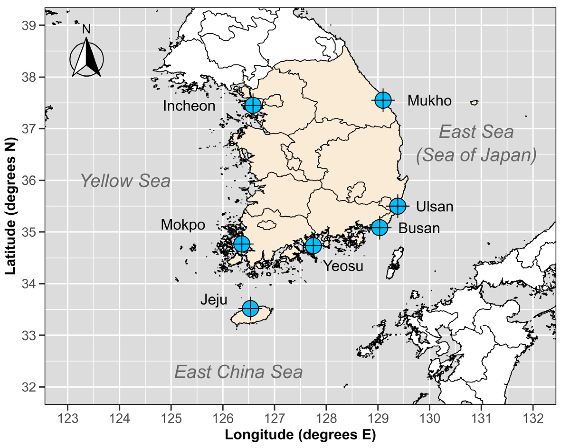
This current study updates the 2019 Assessment with the important benefit of extending the data coverage by a further 7 years to the end of 2025. The results provide improved estimates of real-time mean sea-level velocity at each of the primary tide gauge recording facilities around the Korean Peninsula (Incheon, Mokpo, Busan, Jeju, Mukho, Ulsan and Yeosu) (refer to Figure 1) with improved understanding of associated VLM and updated assessment of trend rates in the surrounding sea margins (Yellow Sea, East China Sea and East Sea (Sea of Japan)) from improved satellite altimetry.
Table 1. Summary of the primary tide gauge and satellite altimeter data used in this study.
PSMSL IDLocationStart (yr)End (yr)Length (yr)CMEMS Grid
(East) 1
CMEMS Grid
(North) 1
956Incheon1960202565126.062537.4375
954Mokpo1960202565125.687534.9375
1066Jeju1964202561126.562533.8125
1155Yeosu1966202559128.062534.5625
955Busan1960202565129.312534.9375
997Ulsan1962202563129.687535.3125
1108Mukho1965202560129.437537.6875
Figure 1 provides plan location details. 1 Satellite altimetry grid point used for VLM analysis (0.125 × 0.125-degree grid, refer to Section 2).
The results presented in this paper provide an improved regional understanding of sea-level rise around the Korean Peninsula to better identify emerging trends of significance and key vulnerabilities to aid relevant policy development, risk mitigation planning and adaptation endeavours.

2. Materials and Methods

This paper seeks to update the 2019 Assessment [12] utilising updated data from the same sources and applying the same methodologies to isolate and determine the trend of MSL and to estimate VLM at the primary tide gauge sites noted in Figure 1. To avoid unnecessary duplication, only a brief description of the key data and relevant methods are described below. For more specific details regarding analytical workflows, including missing data treatment and parameterization of the SSA decomposition procedure, readers are referred to Watson and Lim (2020) [12].

2.1. Data

Annual and monthly average data for each of the primary tide gauge stations has been sourced from the Permanent Service for Mean Sea Level (PSMSL) [15,16] to undertake the MSL trend analysis and VLM assessment, respectively (refer to Table 1 for further details). Specifically, only the PSMSL’s Revised Local Reference (RLR) time series are used for analysis. These data were available to the end of 2024. The data custodian (Korea Hydrographic and Oceanographic Agency (KHOA)) kindly facilitated extending the data to the end of 2025 for the purposes of this study.
Satellite altimetry data from the sea margins surrounding the Korean Peninsula have been sourced from the Copernicus Marine Service (CMS) forming part of the Copernicus Programme which is the European Union’s Earth Observing Programme [17]. Specifically, two separate altimetry datasets have been used for differing purposes. Monthly average time series of 0.125° × 0.125° gridded sea-level anomalies (SLAs) spanning the timeframe from 1 January 1993 to 2 August 2025 have been used in the determination of VLM based on trends from differenced altimetry–tide gauge techniques (ALT-TG, refer to Section 2.3 below for further details). The Copernicus Marine Service product ID is known as SEALEVEL_GLO_PHY_L4_MY_008_047 [18].
The other CMS product used in this study is the 0.25° × 0.25° gridded global ocean SLA trends spanning the period from 20 February 1999 to 10 November 2024 to assess emerging trends in the sea margins surrounding the Korean Peninsula (Yellow Sea, East Sea (Sea of Japan) and East China Sea) [19].

2.2. Estimating MSL (or Trend) from Tide Gauge Records

The data-adaptive spectral technique of Singular Spectrum Analysis (SSA) has been demonstrated to be a very effective tool in isolating time-varying trend signals from complex and noisy time series data [20,21,22,23,24,25] and is proven to be highly efficient in isolating the MSL signal from long tide gauge records [26]. 1D-SSA, using the maximum embedding dimension available for each time series, has been specifically optimised for efficiently estimating MSL from annual average tide gauge data [14] and applied in a range of national sea-level rise assessments (e.g., Australia [27], the USA [28] and South Korea [12]).
The MSL trend can be estimated by aggregating components from a 1-D SSA decomposition of annual averages using frequency thresholding [29] to capture components where more than 50% of the relative spectral energy exceeds the 50 yr frequency band (i.e., 0–0.02 cycles per yr) [30]. The application of a simple cubic smoothing spline [31,32] to the isolated trend permits estimates of time-varying velocity and acceleration in “relative” MSL over the course of the data record.
The abovementioned procedures (including the estimation of errors) are conveniently automated via the “msltrend” extension package [33] in the R programming language for statistical computing (Version 4.4.3) [34]. More detail on the parameterisation of the SSA decomposition approach, fitting of the smooth spline and error handling are specified in the 2019 Assessment by Watson and Lim [12]. The associated scripting code used to undertake all analysis procedures described above are available upon request to the corresponding author.

2.3. Estimating VLM at Tide Gauge

The so-called “ALT-TG” approach [35,36] has been applied to estimate the VLM at the site of each of the primary tide gauges considered in this study. VLM is simply estimated through linear regression of the difference between the respective monthly averages of the SLA altimetry product at the nearest available grid point to the tide gauge no closer than 30 km from the open coast and the “relative” monthly tide gauge record. The timeframe of common coverage between the respective datasets is January 1993 to July 2025. Estimated errors are simply derived from a least squares fitted model.

2.4. Comparison of Regional Sea-Level Trends

The 2019 Assessment provided mapping and assessment of regional gridded altimetry sea-level trends around the sea margins of the Korean Peninsula. The CMS gridded trend estimates of SLA spanned the time horizon extending from September 1992 to May 1999, with no adjustment to these trends for glacial isostatic adjustment (GIA). Increasingly modern sea-level studies involving satellite altimetry have been correcting for the GIA influence. These corrections provide a more accurate reflection of the true rate of sea-level rise as the ocean basins are getting larger as sea-level increases whilst at the same time, the water volume is expanding from thermosteric effects [37]. The most recent gridded SLA trend maps provided by CMS are applied to the same spatial grid (0.25° × 0.25°) but importantly, are now supplied in a form that has corrections for GIA already applied and built into the supplied dataset per Spada and Melini (2019) [38]. Unfortunately, the GIA corrections applied are not provided with the recent SLA trend mapping and were not able to be provided by CMS.
Therefore, to provide a baseline comparative assessment between the altimetry trends provided in the 2019 Assessment and the more recently available SLA trend mapping, the recent dataset requires to be “uncorrected” for the GIA applied. An estimate of GIA corrections on a coarser spatial resolution grid (1° × 1°) to the CMS altimetry product have been provided for this research by Professor Giorgio Spada, University of Bologna, Italy (personal communication, 10 August 2025). In general terms, the global average GIA correction for altimetry data is around ≈−0.3 mm/yr [37]. Within the regional sea margins around the Korean Peninsula (refer to spatial reference boxes, Section 3.2), the average 1-degree gridded GIA solutions are of the opposite sign and around ≈0.50 mm/yr.
The analysis provided in this paper is limited to a comparative assessment of SLA trend rates between the two datasets within the spatial reference boxes advised (refer to Section 3.2). The adjustments applied to estimate the reduction owing to the GIA correction in the latter dataset is simply an average of the 1-degree gridded GIA values bounded within the same spatial reference boxes (refer to Section 3.2). It is important to note that as GIA values in the sea margins around the Korean Peninsula are positive, the correction applied to the satellite altimetry data (by CMS) result in the trend rate being reduced. To remove the correction, these trend rates now must be increased by the GIA estimate.

3. Results

The presentation of all analysis and results depicting scientific error margins are advised at the 95% confidence level (CL) unless specifically noted otherwise. Results have been partitioned into those relating to the tide gauge data analysis and those relating to satellite altimetry in the sea margins surrounding the Korean Peninsula.

3.1. Tide Gauge Results

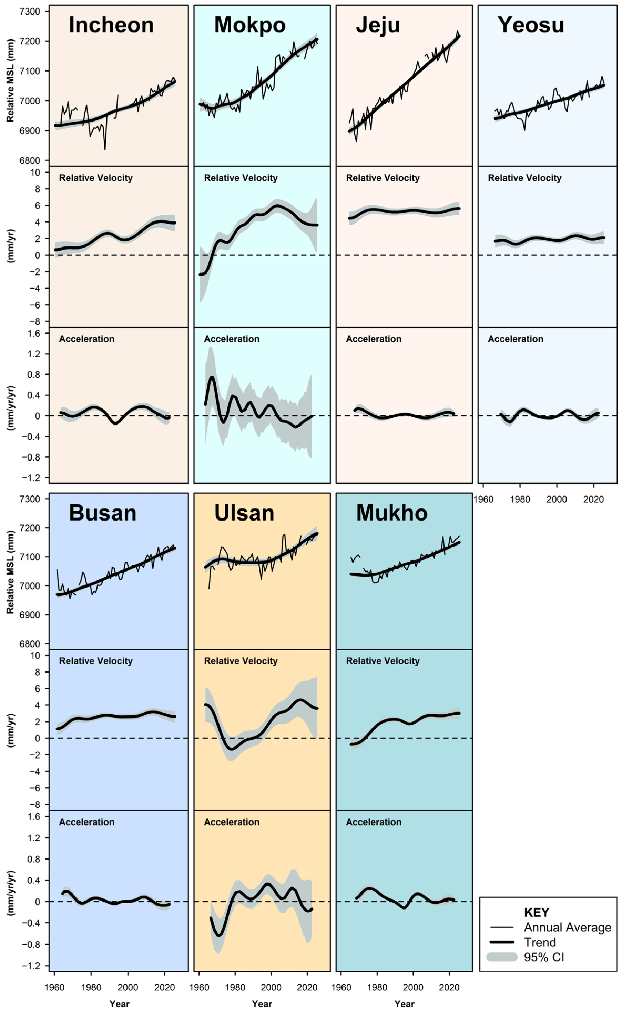
The results of the SSA decomposition of the annual average tide gauge data for each of the seven primary tide gauges are presented in Figure 2. Each station record contains a three-panel plot depicting the time-varying “relative” MSL in the top panel, along with the associated velocity (middle panel) and acceleration (bottom panel).
It is evident that despite fluctuations over time, the MSL (trend) has continued to increase with the highest MSL being recorded at each station during 2025 (most recent data point). The associated “relative” velocities at each station show marked variability over time with several exhibiting a general tendency of increase over time to present (e.g., Incheon, Busan, Mukho), suggesting the presence of an acceleration to do so, albeit at a rate indistinguishable from zero (within experimental error margins). Jeju and Yeosu exhibit a trend of largely constant “relative” velocity over time with no measurable acceleration in MSL rise to date.
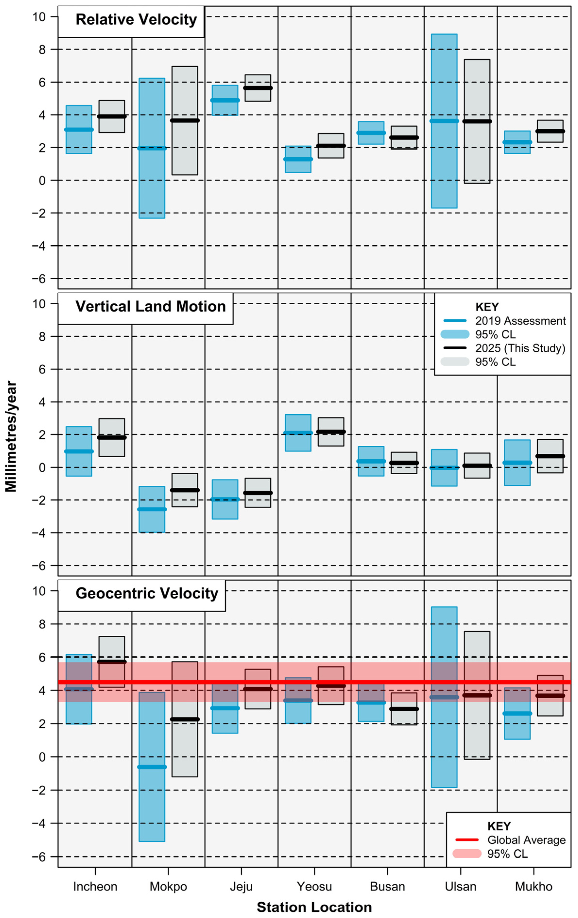
Figure 3 provides a summary of the “relative” velocity (top panel), VLM (centre panel) and “geocentric” (i.e., corrected for VLM) velocity (bottom panel) at each primary tide gauge location for 2025 (this study). This figure also provides direct comparative results for the 2019 Assessment [12] highlighted in blue, permitting changes to be observed in the respective parameters with the addition of a further 7 years of data.
These additional years of data permit both improved SSA resolution of the low-frequency “relative” MSL trend (and associated velocity) and VLM estimates via the ALT-TG technique. This is confirmed with a 22% reduction in the 95% CL between the average “relative” velocity from the current study compared to the previous (2019) study (top panel, Figure 3). Similarly, there is a 26% reduction in the 95% CL between the average VLM estimates between the current study and 2019 Assessment (middle panel, Figure 3).
The “relative” rate of MSL rise (top panel, Figure 3) in 2025 is above 2 mm/yr at all seven tide gauge stations and above 3.5 mm/yr at Incheon, Mokpo, Jeju and Ulsan. The highest rate (5.6 mm/yr) was measured at Jeju. Some five of the seven stations recorded an increase in the rate of “relative” MSL rise compared to the 2019 Assessment (Incheon, Mokpo, Jeju, Yeosu and Mukho) at an average increase of ≈0.9 mm/yr. Ulsan remained unchanged, whilst Busan experienced a small decrease of 0.3 mm/yr compared to the 2019 Assessment.
VLM differences between the current and 2019 Assessment remain quite consistent with the extension of 7 years of data, with five of the seven stations (Jeju, Yeosu, Busan, Ulsan and Mukho) exhibiting differences in VLM estimates between the respective studies of less than 0.4 mm/yr (middle panel, Figure 3). At the 95% CL, Incheon and Yeosu exhibit a clear trend of uplift at average rates of ≈2 mm/yr whilst Mokpo and Jeju exhibit a subsidence trend at average rates ≈ 1.5 mm/yr. At the 95% CL, the tidal stations at Busan, Ulsan and Mukho continue to exhibit no trend of VLM from these analyses.
When the “relative” rate of MSL rise is corrected for VLM, the “geocentric” rate of MSL rise (bottom panel, Figure 3) follows similar trends in that increases have been experienced at all stations except for Busan and Ulsan since the 2019 Assessment. Some five of the seven stations (Incheon, Jeju, Yeosu, Ulsan and Mokpo) exhibit trends in current “geocentric” MSL rise at or above 3.7 mm/yr, with Incheon the highest at 5.7 mm/yr.
The bottom panel of Figure 3 superimposes an estimate of global MSL rise (in red) proposed by Hamlington et al., (2024) [39]. At the 95% CL, the rate of “geocentric” MSL rise at all seven stations around the Korean Peninsula accords with this recently published estimate of global-averaged MSL rise (4.5 ± 1.2 mm/yr).

3.2. Altimetry Results

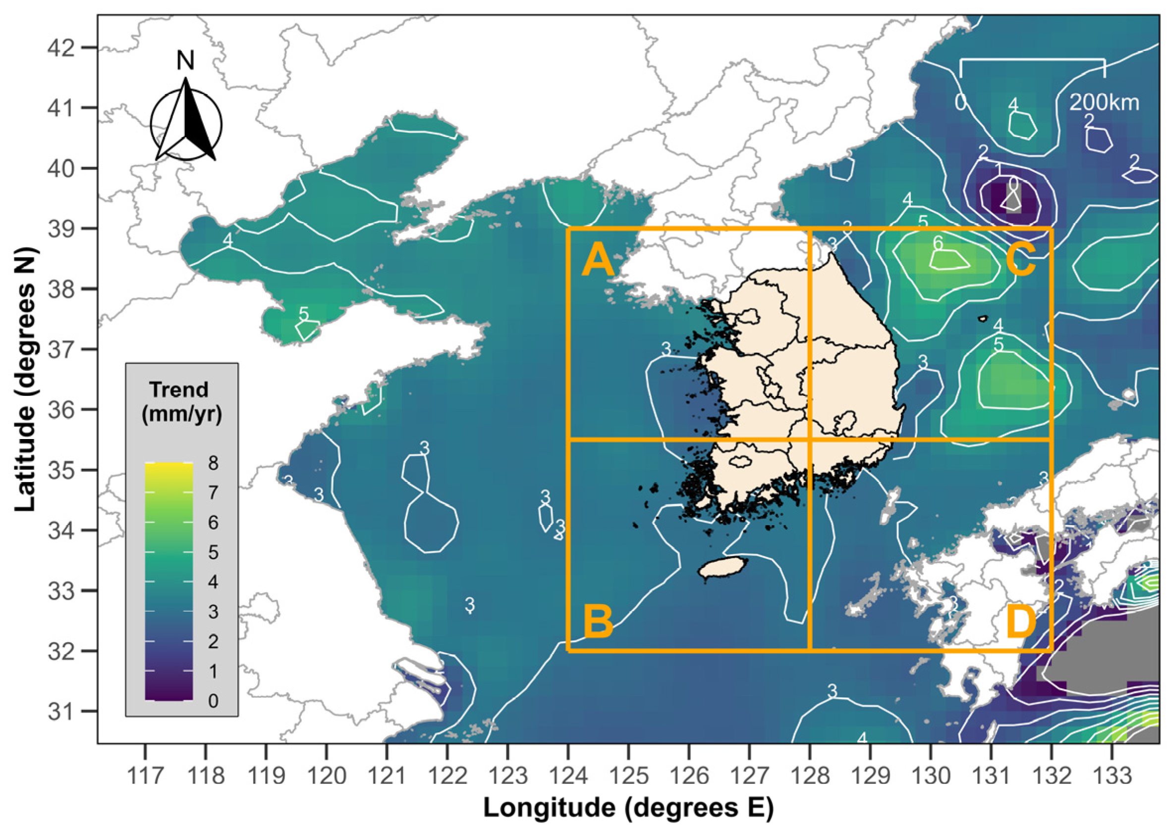
Figure 4 provides a contour map of trends in ocean SLA around the Korean Peninsula based on satellite altimetry from the CMS. These trends are based on linear regression of the timespan between 20 February 1999 and 19 November 2024. The trends were provided having been automatically corrected for GIA based on Spada and Melini (2019) [38].
From Figure 4, two distinct areas of elevated SLA trends (above 5 mm/yr) continue to expand within the East Sea (Sea of Japan) above ≈36° N (refer to Panel C).
In the prior 2019 Assessment by Watson and Lim [12], the CMS regional map of SLA trends was not corrected for GIA. Therefore, to directly compare the previous trends to the recently updated trends (which have been corrected by CMS for GIA), the advised trends need to be converted using the GIA corrections of Spada and Melini (2019) [38].
One-degree grids of GIA corrections provided by Professor Giorgio Spada, University of Bologna, Italy (personal communication, 10 August 2025), have been used to permit direct comparison between the 2019 CMS gridded SLA trends and the updated CMS gridded product.
Table 2 provides a comparison of SLA trends from 2019 and 2024 within the respective boxes highlighted in Figure 4 (A, B, C and D). Once the 2024 altimetry has been adjusted for GIA to be directly comparable to the altimetry trends advised in 2019, a small average increase in trend rates of ≈1% is evident. Similarly, areas A, B and C exhibit average increases in trend rates of 2.5%, 2.9% and 10.8%, respectively, whilst area D indicates a small decrease in average trend rates of 1.8% between 2019 and 2024 altimetry.
In the previous 2019 Assessment, the highest gridded altimetry trends were evident in area C within the margins of the East Sea (Sea of Japan). The current (2024) altimetry trends show the highest average increases in area C at nearly 11% compared to 2019, highlighting the continued rate of rise in sea surface heights in this area, at much higher rates than the regional average.
Area C houses the Tsushima Warm Current (TWC) which delivers a combination of warm saline waters from the Kuroshio Current mixed with freshwater from the East China Sea through the Tsushima Strait into the East Sea (Sea of Japan) [40]. The Kuroshio Current is a major western boundary current controlled by the North Pacific Gyre bringing warm tropical waters from the Indo-Pacific Warm Pool to Japan and exerting a major control on the climate of Northeast Asia [40]. The highest gridded altimetry trends are within the pathway of the TWC, indicating the primary driver is most likely due to thermosteric influences associated with global warming. Numerous scientific publications have advised the significant warming of the waters of the East Sea (Sea of Japan) over several decades (e.g., [41,42,43]), in line with climate change projections.
Substantial spatial differences in SLA trends in the sea margins around the Korean Peninsula are principally associated with the teleconnections associated with ocean heat content conveyors (or major ocean currents) being the Kuroshio Current and northern branches through the Tsushima Strait to feed the Tsushima Warm Current in the East Sea (Sea of Japan). The highest SLA trend rates observed in area C exceed 6 mm/yr and are well above the global average rate. These (and higher) rates are evident within other similar warm current streams, globally distributing warm waters from the equator along the eastern boundary of continents towards the poles (e.g., East Australian Current, Kuroshio Current, Gulf Stream, Agulhas and Brazil Currents) [11].
The likelihood of projected climate change continuing to influence the distribution of heat energy around the Korean Peninsula and how these thermosteric ocean processes will impact sea-level rise rates around associated foreshores should continue to be an active focus of future research endeavours.

4. Discussion

4.1. Limitations of Mean Sea-Level Analysis

In any scientific study, it is important to be cognizant of inherent limitations. The earliest available datasets from primary tide gauges around the Korean Peninsula date back to 1960 (Incheon, Mokpo and Busan). At 65 years in length, these datasets remain comparatively short for trying to resolve the MSL trend and associated velocities and accelerations. Optimal minimum length tide gauge datasets for MSL research are generally considered to be in the vicinity of 75–80 years [13,14] to permit adequate separation of the anharmonic and slowly varying trend signal (driven ostensibly by climate change) from the other coexistent dynamic geophysical and meteorological forcings and noise.
It is relevant that with an additional 7 years of tide gauge data available beyond the previous 2019 Assessment that the SSA decomposition resulted in stronger separation of individual components in the low-frequency (or “trend-like”) bandwidth, resulting in reduced error margins for the determined MSL trend and associated velocities and accelerations. This will improve further as the datasets continue to lengthen. Notwithstanding limitations imposed by the length of available tide gauge data for MSL analysis, this study has used state-of-the-art analysis techniques to maximise the information that can be ascertained from the information available.

4.2. Limitations of VLM Analysis

The ALT-TG technique to estimate VLM at the primary tide gauges is a valuable tool for assessing “geocentric” MSL rise around the Korean Peninsula. The additional 7 years of data extends the length of the altimetry database by nearly 25% and correspondingly, the 95% error margins for the respective VLM estimates have reduced on average by around 26%, demonstrating the importance of lengthening data availability. It should however be remembered that the ALT-TG technique is considered an alternative or proxy methodology to estimate VLM in the absence of the availability of more precise, robust, collocated continuous GPS technology. It is evident that some form of GPS measuring equipment has been available near the majority of the primary tide stations used in this study from as early as 2005 (Incheon) through to 2011 (Yeosu), based on a 2019 National Report to the UNESCO Intergovernmental Oceanographic Commission on the status of tide gauges managed by the Republic of Korea [44]. Minimum recommended standards for robust VLM estimates at tide gauges from continuous GPS require the instrument to be sited no further than 1 km from the tide gauge [45] and for continuous measurements to generally exceed 10 years in length [46,47]
Other techniques such as Interferometric Synthetic Aperture Radar (InSAR) and Persistent Scatterer Interferometry (PS-InSAR) have also been applied to estimate VLM at tide gauges around the Korean Peninsula [4,48] with relevant VLM estimates compared to those obtained from this study (refer to Table 3).
The InSAR analysis of Vadivel et al., (2021) [48] was based on the use of C-band Sentinel-1 A/B Synthetic Aperture Radar (SAR) data acquired during a 6 yr period (2014–2020). The PS-InSAR analysis of Adhikari et al., (2025) [4] was also based on multi-temporal C-band Sentinel-1 data acquired during a 6 yr period (2017–2023). Both SAR applications require significant expert interpretation and processing workflows to estimate VLM.
Table 3 highlights clear differences between VLM estimates obtained from the respective InSAR, PS-InSAR and ALT-TG techniques, noting that only three sites (Incheon, Mokpo and Yeosu) are covered by all approaches. Notwithstanding, there are also several instances of close agreement, for example, Incheon (InSAR and ALT-TG), Mokpo (PS-InSAR and ALT-TG), Jeju (InSAR and ALT-TG), Yeosu (InSAR and PS-InSAR) and Busan (PS-InSAR and ALT-TG).
Differences in VLM estimates between methods could result from the small (6 yr) time windows used by the InSAR and PS-InSAR approaches, noting the 6 yr time windows are different, compared to the much longer data analysis timeframe of the ALT-TG approach (>30 years).
Vadivel et al., (2021) advise that a major limitation of the InSAR approach to estimating VLM is when the tide gauge stations are located in areas such as dense vegetation terrain; unstable coherent targets such as containers in the port often lose the stable coherent targets, leading to phase unwrapping errors [48]. Adhikari et al., (2025) [4] advise that VLM derived from ALT-TG and PS-InSAR generally remained within uncertainty bounds, with exceptions at Incheon, Ulsan, Mukho, and Yeosu. It was noted that these differences highlight the critical influence of persistent scatterer point (PSP) selection near tide gauges when determining average VLM [4].
Notwithstanding the abovementioned issues, the InSAR and PS-InSAR approaches offer an alternative technique to estimate VLM where it can also be demonstrated that the associated standard error in the estimate can be reduced to the order of 0.5 mm/yr which has been established as a pre-requisite for international scientific sea-level studies [45,47]. Similarly, the authors note that the InSAR technique offers an alternative approach in the absence of available in situ GNSS, particularly as the volume of SAR data continues to grow rapidly with Sentinel-1 A/B [48] and other current and future missions with increasingly advanced capabilities [49].
As previously discussed, the ALT-TG technique offers an alternative method of VLM estimation that has been validated against a global repository of tide gauges with collocated GNSS receivers [36]. The technique can be readily applied around any jurisdiction with monthly average tide gauge data extending back over the altimetry era (≈1993). For most locations around the globe, the requisite data (gridded sea surface altimetry and monthly tide gauge measurements) are publicly available for research and scientific purposes with a comparatively simple analysis procedure involved to estimate VLM. The length of data used to estimate VLM using the ALT-TG approach now generally exceeds 30 years. In the case of the current study, standard errors for VLM estimation at each of the primary tide gauge locations are ≈0.5 mm/yr (or less).
The estimates of VLM error at Incheon and Mukho are higher and likely less reliable as advised previously in Watson and Lim (2020) [12] whereby satellite altimeters perform very well over the open ocean; however, a number of issues arise in the vicinity of land, related to poorer geophysical corrections and artefacts in the altimeter reflected signals linked to the presence of land within the instrument footprint [50]. Sea state bias corrections, as well as tides and the ocean response to atmospheric forcings, have been tailored to deep ocean conditions [51], thereby substantially degrading the accuracy of the measured sea surface estimate closer to the coast in areas where large tidal amplitudes and waves are routinely encountered. This is particularly the case for the western coast of Korea, where tidal ranges up to 10 m are experienced [52] and a strong feature of the south-western coastline is the archipelago of micro and small islands.
Understanding VLM at the site of the tide gauge is critical to enhancing the scientific understanding of sea-level rise along developed coastlines and providing reliable, robust estimates of “geocentric” mean sea level. Knowledge of where landforms are subsiding highlights areas where rising sea levels, storm surges and oceanic (or saltwater) intrusion will be critically exacerbated. Estimating VLM is best achieved through the collocation of GNSS receivers and tide gauges over time. Although it is evident that the primary tide gauges around the Korean Peninsula are equipped with some form of continuous GPS/GNSS [44], these data were not publicly available in key international GNSS repositories which facilitate scientific research into rising sea levels (e.g., Système d’Observation du Niveau des Eaux Littorales (SONEL), Nevada Geodetic Laboratory (NGL), International GNSS Service (IGS)).
Due to the criticality of understanding VLM at the primary tide gauge sites around the Korean Peninsula, it is strongly recommended that a more comprehensive analysis of VLM at each site is considered comparing each of the methods available (GNSS, InSAR and ALT-TG) as a matter of scientific priority moving forward and that where GNSS data is being captured, it is made more broadly available to international repositories to facilitate improved scientific understanding of the evolving threat posed by rising sea levels, exacerbated by subsiding land margins.

5. Conclusions

Surrounded by the Yellow Sea to the west, East Sea (Sea of Japan) to the east and the East China Sea to the south, the Korean Peninsula is critically exposed to impacts associated with rising MSL. Existing threats associated with coastal hazards (e.g., typhoon-driven storm surges, shoreline and beach erosion, oceanic inundation, saltwater flooding, etc.) will all be worsened by continually rising MSL associated with a changing global climate.
This study importantly updates the 2019 Assessment [12] using data sourced to the end of 2025. With the longest tidal gauge station record around the Korean Peninsula at ≈65 years, these records are comparatively short for isolating high-resolution MSL trend estimates. Therefore, the addition of 7 years of data since the previous comprehensive assessment is invaluable to improving the regional understanding of current and emerging trends of this significant phenomenon, whilst benchmarking against global climate forecast models.
These additional years of data have improved the robustness of all analytical procedures applied for both MSL trend and VLM estimates with a general reduction in the associated error estimates of ≈25% when compared to the 2019 Assessment.
From the current analysis, some five of the seven primary tide gauge stations have recorded an increase in the rate of “relative” MSL rise compared to the previous study (Incheon, Mokpo, Jeju, Yeosu and Mukho). VLM rates remain comparatively consistent with Incheon and Yeosu, continuing to exhibit a trend of uplift (≈2 mm/yr) whilst Mokpo and Jeju exhibit trends of subsidence (≈1.5 mm/yr).
Having corrected for VLM, only Busan and Ulsan have not experienced an increase in the rate of “geocentric” MSL rise since the 2019 Assessment. At the 95% CL, the current rate of “geocentric” MSL rise at all stations accord with recent published estimates of the rate of global-averaged MSL rise. Given the criticality of VLM to understanding “geocentric” mean sea-level trends around the Korean Peninsula, it is strongly recommended to undertake detailed comparative analysis at each of the primary tide gauge sites using GNSS, InSAR and ALT-TG techniques. It is also recommended that existing GNSS data in proximity to these tide gauges is made available to publicly accessible global data repositories established to enable GNSS data to augment scientific research into sea-level rise (e.g., SONEL, NGL, IGS).
From consideration of satellite altimetry of the sea margins around the Korean Peninsula, there has been a small (≈1%) increase in the average regional trend of SLA compared to the 2019 Assessment. The most significant trend estimates in SLA continue to increase in margins of the East Sea (Sea of Japan) between 35° N and 40° N with increases of around 11% in the rate of trend above the 2019 Assessment due principally to thermosteric influences associated with flows from the Tsushima Warm Current. Continuing to understand current and projected climate change impacts and how ocean heat energy will be directed via the Kuroshio Current and northern branches through the Tsushima Strait to feed the Tsushima Warm Current in the East Sea (Sea of Japan) should be a focus of future research initiatives. The likelihood of projected climate change continuing to influence the distribution of heat energy around the Korean Peninsula and how these thermosteric ocean processes will impact sea-level rise rates around associated foreshores will prove critical for future planning and mitigation endeavours.
It is of critical importance that these types of regional MSL analyses continue to be updated every 5 years or so to leverage both the benefits of lengthening data and improved analyses and scientific understanding about climate change and its role in influencing sea-level rise.

Author Contributions

Conceptualization, P.J.W. and H.-S.L.; methodology, P.J.W.; software, P.J.W.; formal analysis, P.J.W.; data curation, P.J.W. and H.-S.L.; writing—original draft preparation, P.J.W.; review and editing, H.-S.L.; supervision, H.-S.L.; project administration, H.-S.L. All authors have read and agreed to the published version of the manuscript.

Funding

This research received no external funding.

Data Availability Statement

The data presented in this study are openly available from the Permanent Service for Mean Sea Level (PSMSL) at https://www.psmsl.org/data/obtaining/ (accessed on 26 April 2026), reference number [8].

Conflicts of Interest

The authors declare no conflicts of interest.

References

  1. Lee, H.; Calvin, K.; Dasgupta, D.; Krinner, G.; Mukherji, A.; Thorne, P.; Trisos, C.; Romero, J.; Aldunce, P.; Barret, K.; et al. IPCC, 2023: Climate Change 2023: Synthesis Report, Summary for Policymakers. Contribution of Working Groups I, II and III to the Sixth Assessment Report of the Intergovernmental Panel on Climate Change; Lee, H., Romero, J., Eds.; IPC: Geneva, Switzerland, 2023. [Google Scholar]
  2. IPCC; Masson-Delmotte, V.; Zhai, P.; Pirani, A.; Connors, S.L.; Péan, C.; Berger, S.; Caud, N.; Chen, Y.; Goldfarb, L.; et al. Climate Change 2021: The Physical Science Basis. Contribution of Working Group I to the Sixth Assessment Report of the Intergovernmental Panel on Climate Change; IPCC: Geneva, Switzerland, 2021. [Google Scholar]
  3. Park, Y.; Jung, B.; Kim, R. Flood Risk Assessment for Coastal Cities Considering Sea Level Rise Due to Climate Change. J. Korean Soc. Hazard Mitig. 2020, 20, 323–332. [Google Scholar] [CrossRef] [Scilit]
  4. Adhikari, M.D.; Song, M.S.; Yum, S.G. The Impact of Climate Change and Localized Land Subsidence along the Korean Peninsula Coastline: An Overview of Future Coastal Inundation and Vulnerability. Int. J. Appl. Earth Obs. Geoinf. 2025, 144, 104894. [Google Scholar] [CrossRef] [Scilit]
  5. Lee, J.S.; Choi, H. Il Development and Implementation of an Assessment Framework for Coastal Flood Vulnerability. J. Korean Soc. Hazard Mitig. 2018, 18, 291–299. [Google Scholar] [CrossRef] [Scilit]
  6. Park, S.J.; Lee, D.K. Prediction of Coastal Flooding Risk under Climate Change Impacts in South Korea Using Machine Learning Algorithms. Environ. Res. Lett. 2020, 15, 094052. [Google Scholar] [CrossRef] [Scilit]
  7. Choi, M.; Kim, M. Estimating Direct and Indirect Damage to Industrial Facilities from Coastal Flooding: Case of Ulsan, Korea. J. Korean Soc. Hazard Mitig. 2024, 24, 257–265. [Google Scholar] [CrossRef] [Scilit]
  8. Das Adhikari, M.; Park, S.; Yum, S.G. Coastal Vulnerability to Extreme Weather Events: An Integrated Analysis of Erosion, Sediment Movement, and Land Subsidence Based on Multi-Temporal Optical and SAR Satellite Data. J. Environ. Manag. 2025, 374, 124025. [Google Scholar] [CrossRef] [Scilit]
  9. Govorcin, M.; Bekaert, D.P.S.; Hamlington, B.D.; Sangha, S.S.; Sweet, W. Variable Vertical Land Motion and Its Impacts on Sea Level Rise Projections. Sci. Adv. 2025, 11, eads8163. [Google Scholar] [CrossRef] [Scilit] [PubMed]
  10. Shirzaei, M.; Freymueller, J.; Törnqvist, T.E.; Galloway, D.L.; Dura, T.; Minderhoud, P.S.J. Measuring, Modelling and Projecting Coastal Land Subsidence. Nat. Rev. Earth Environ. 2021, 2, 40–58. [Google Scholar] [CrossRef] [Scilit]
  11. Fox-Kemper, B.; Hewitt, H.T.; Xiao, C.; Aðalgeirsdόttir, G.; Drijfhout, S.S.; Edwards, T.L.; Golledge, N.R.; Hemer, M.; Kopp, R.E.; Krinner, G.; et al. Ocean, Cryosphere and Sea Level Change. In Climate Change 2021: The Physical Science Basis. Contribution of Working Group I to the Sixth Assessment Report of the Intergovernmental Panel on Climate Change; Masson-Delmotte, V., Zhai, P., Pirani, A., Connors, S.L., Péan, C., Berger, S., Caud, N., Chen, Y., Goldfarb, L., Gomis, M.I., et al., Eds.; Cambridge University Press: Cambridge, UK; New York, NY, USA, 2021; pp. 1211–1362. [Google Scholar]
  12. Watson, P.J.; Lim, H.S. An Update on the Status of Mean Sea Level Rise around the Korean Peninsula. Atmosphere 2020, 11, 1153. [Google Scholar] [CrossRef] [Scilit]
  13. Houston, J.R.; Dean, R.G. Effects of Sea-Level Decadal Variability on Acceleration and Trend Difference. J. Coast. Res. 2013, 290, 1062–1072. [Google Scholar] [CrossRef] [Scilit]
  14. Watson, P.J. Improved Techniques to Estimate Mean Sea Level, Velocity and Acceleration from Long Ocean Water Level Time Series to Augment Sea Level (and Climate Change) Research. Ph.D. Thesis, University of New South Wales, Sydney, NSW, Australia, 2018. [Google Scholar]
  15. Holgate, S.J.; Matthews, A.; Woodworth, P.L.; Rickards, L.J.; Tamisiea, M.E.; Bradshaw, E.; Foden, P.R.; Gordon, K.M.; Jevrejeva, S.; Pugh, J. New Data Systems and Products at the Permanent Service for Mean Sea Level. J. Coast. Res. 2013, 29, 493. [Google Scholar] [CrossRef] [Scilit]
  16. PSMSL Permanent Service for Mean Sea Level. Available online: https://www.psmsl.org/data/obtaining/ (accessed on 1 December 2025).
  17. European Union Copernicus Program. Copernicus Marine Website. Available online: https://marine.copernicus.eu/ (accessed on 20 December 2025).
  18. Copernicus Marine Service. Global Ocean Gridded L 4 Sea Surface Heights And Derived Variables Reprocessed 1993 Ongoing. Sea Surface Anomalies. Available online: https://data.marine.copernicus.eu/product/SEALEVEL_GLO_PHY_L4_MY_008_047/ (accessed on 20 January 2026).
  19. Copernicus Marine Service. Global Ocean Mean Sea Level Trend Map from Observations Reprocessing. Available online: https://data.marine.copernicus.eu/product/OMI_CLIMATE_SL_GLOBAL_regional_trends/ (accessed on 20 January 2026).
  20. Broomhead, D.S.; King, G.P. Extracting Qualitative Dynamics from Experimental Data. Phys. D 1986, 20, 217–236. [Google Scholar] [CrossRef] [Scilit]
  21. Vautard, R.; Ghil, M. Singular Spectrum Analysis in Nonlinear Dynamics, with Applications to Paleoclimatic Time Series. Phys. D 1989, 35, 395–424. [Google Scholar] [CrossRef] [Scilit]
  22. Elsner, J.B.; Tsonis, A.A. Singular Spectrum Analysis: A New Tool in Time Series Analysis; Springer Science & Business Media: New York, NY, USA, 2013. [Google Scholar]
  23. Vautard, R.; Yiou, P.; Ghil, M. Singular-Spectrum Analysis: A Toolkit for Short, Noisy Chaotic Signals. Phys. D 1992, 58, 95–126. [Google Scholar] [CrossRef] [Scilit]
  24. Golyandina, N.; Korobeynikov, A.; Zhigljavsky, A. Singular Spectrum Analysis with R; Springer: Berlin/Heidelberg, Germany, 2018; ISBN 9783662573785. [Google Scholar]
  25. Golyandina, N. Particularities and Commonalities of Singular Spectrum Analysis as a Method of Time Series Analysis and Signal Processing. Wiley Interdiscip. Rev. Comput. Stat. 2020, 12, e1487. [Google Scholar] [CrossRef] [Scilit]
  26. Watson, P.J. Identifying the Best Performing Time Series Analytics for Sea Level Research. In Time Series Analysis and Forecasting: Contributions to Statistics; Rojas, I., Pomares, H., Eds.; Springer: Cham, Switzerland, 2016; pp. 261–278. [Google Scholar]
  27. Watson, P.J. Updated Mean Sea-Level Analysis: Australia. J. Coast. Res. 2020, 36, 915–931. [Google Scholar] [CrossRef] [Scilit]
  28. Watson, P.J. Status of Mean Sea Level Rise around the USA (2020). GeoHazards 2021, 2, 80–100. [Google Scholar] [CrossRef] [Scilit]
  29. Alexandrov, T.; Golyandina, N. Automatic Extraction and Forecast of Time Series Cyclic Components within the Framework of SSA. In Proceedings of the 5th St. Petersburg Workshop on Simulation, St. Petersburg, Russia, 26 June–2 July 2005; pp. 45–50. [Google Scholar]
  30. Mann, M.E.; Steinman, B.A.; Miller, S.K. Absence of Internal Multidecadal and Interdecadal Oscillations in Climate Model Simulations. Nat. Commun. 2020, 11, 49. [Google Scholar] [CrossRef] [Scilit] [PubMed]
  31. Greem, P.J.; Silverman, B.E. Nonparametric Regression and Generalized Linear Models; Taylor & Francis: London, UK, 1994. [Google Scholar]
  32. Hastie, T.J. Generalized Additive Models. In Statistical Models in S; Taylor & Francis: Abingdon, UK, 2017; pp. 249–307. [Google Scholar]
  33. Watson, P.J. TrendSLR: Estimating Trend, Velocity and Acceleration from Sea Level Records, Extension Software Package in R Foundation for Statistical Computing. 2019. Available online: https://rdocumentation.org/packages/TrendSLR/versions/1.0 (accessed on 26 April 2026).
  34. R Development Core Team R: A Language and Environment for Statistical Computing. In R Foundation for Statistical Computing Vienna Austria. Available online: https://www.r-project.org/ (accessed on 26 April 2026).
  35. Ostanciaux, É.; Husson, L.; Choblet, G.; Robin, C.; Pedoja, K. Present-Day Trends of Vertical Ground Motion along the Coast Lines. Earth. Sci. Rev. 2012, 110, 74–92. [Google Scholar] [CrossRef] [Scilit]
  36. Watson, P.J. An Assessment of the Utility of Satellite Altimetry and Tide Gauge Data (ALT-TG) as a Proxy for Estimating Vertical Land Motion. J. Coast. Res. 2019, 35, 1131–1144. [Google Scholar] [CrossRef] [Scilit]
  37. Sea Level Research Group University of Colorado What Is Glacial Isostatic Adjustment (GIA), and Why Do You Correct for It? Available online: https://sealevel.colorado.edu/presentation/what-glacial-isostatic-adjustment-gia-and-why-do-you-correct-it (accessed on 1 April 2026).
  38. Spada, G.; Melini, D. SELEN 4 (SELEN Version 4.0): A Fortran Program for Solving the Gravitationally and Topographically Self-Consistent Sea-Level Equation in Glacial Isostatic Adjustment Modeling. Geosci. Model Dev. 2019, 12, 5055–5075. [Google Scholar] [CrossRef] [Scilit]
  39. Hamlington, B.D.; Bellas-Manley, A.; Willis, J.K.; Fournier, S.; Vinogradova, N.; Nerem, R.S.; Piecuch, C.G.; Thompson, P.R.; Kopp, R. The Rate of Global Sea Level Rise Doubled during the Past Three Decades. Commun. Earth Environ. 2024, 5, 601. [Google Scholar] [CrossRef] [Scilit]
  40. Gallagher, S.J.; Kitamura, A.; Iryu, Y.; Itaki, T.; Koizumi, I.; Hoiles, P.W. The Pliocene to Recent History of the Kuroshio and Tsushima Currents: A Multi-Proxy Approach. Prog. Earth Planet. Sci. 2015, 2, 17. [Google Scholar] [CrossRef] [Scilit]
  41. Kim, K.; Kim, K.R.; Min, D.H.; Volkov, Y.; Yoon, J.H.; Takematsu, M. Warming and Structural Changes in the East (Japan) Sea: A Clue to Future Changes in Global Oceans? Geophys. Res. Lett. 2001, 28, 3293–3296. [Google Scholar] [CrossRef] [Scilit]
  42. Na, H.; Kim, K.Y.; Chang, K.I.; Park, J.J.; Kim, K.; Minobe, S. Decadal Variability of the Upper Ocean Heat Content in the East/Japan Sea and Its Possible Relationship to Northwestern Pacific Variability. J. Geophys. Res. Oceans 2012, 117, 1–11. [Google Scholar] [CrossRef] [Scilit]
  43. Hayashi, M.; Shiogama, H.; Ogura, T. The Contribution of Climate Change to Increasing Extreme Ocean Warming Around Japan. Geophys. Res. Lett. 2022, 49, e2022GL100785. [Google Scholar] [CrossRef] [Scilit]
  44. Korea Hydrographic and Oceanographic Agency (KHOA). National Report of Korea; KHOA: Busan, Republic of Korea, 2019. [Google Scholar]
  45. Wöppelmann, G.; Aarup, T.; Schoene, T. An Inventory of Collocated and Nearly-Collocated CGPS Stations and Tide Gauges; SONEL Université de La Rochelle: La Rochelle, France, 2007. [Google Scholar]
  46. Snay, R.; Cline, M.; Dillinger, W.; Foote, R.; Hilla, S.; Kass, W.; Ray, J.; Rohde, J.; Sella, G.; Soler, T. Using Global Positioning System-Derived Crustal Velocities to Estimate Rates of Absolute Sea Level Change from North American Tide Gauge Records. J. Geophys. Res. Solid Earth 2007, 112, 1–11. [Google Scholar] [CrossRef] [Scilit]
  47. Masson, C.; Mazzotti, S.; Vernant, P. Precision of Continuous GPS Velocities from Statistical Analysis of Synthetic Time Series. Solid Earth 2019, 10, 329–342. [Google Scholar] [CrossRef] [Scilit]
  48. Vadivel, S.K.P.; Kim, D.J.; Jung, J.; Cho, Y.K.; Han, K.J. Monitoring the Vertical Land Motion of Tide Gauges and Its Impact on Relative Sea Level Changes in Korean Peninsula Using Sequential SBAS-InSAR Time-Series Analysis. Remote Sens. 2020, 13, 18. [Google Scholar] [CrossRef] [Scilit]
  49. Zakharov, I.; Power, D.; McGuire, P.; Völker, M.; Kim, J.H.; Emanuelli, M.; Chamberland, J.; Stott, M.; Warren, S.; Janoth, J.; et al. Next-Generation C-Band SAR Mission: Design Concept for Earth Observation Service Continuity. Remote Sens. 2025, 17, 3761. [Google Scholar] [CrossRef] [Scilit]
  50. Gommenginger, C.; Thibaut, P.; Fenoglio-Marc, L.; Quartly, G.; Deng, X.; Gómez-Enri, J.; Challenor, P.; Gao, Y. Retracking Altimeter Waveforms near the Coasts a Review of Retracking Methods and Some Applications to Coastal Waveforms. In Coastal Altimetry; Springer: Berlin/Heidelberg, Germany, 2011. [Google Scholar]
  51. Roblou, L.; Lamouroux, J.; Bouffard, J.; Lyard, F.; Le Hénaff, M.; Lombard, A.; Marsaleix, P.; De Mey, P.; Birol, F. Post-Processing Altimeter Data towards Coastal Applications and Integration into Coastal Models. In Coastal Altimetry; Springer: Berlin/Heidelberg, Germany, 2011. [Google Scholar]
  52. Hwang, S.J.; Jo, C.H. Tidal Current Energy Resource Distribution in Korea. Energies 2019, 12, 4380. [Google Scholar] [CrossRef] [Scilit]
Figure 1. Location diagram highlighting the position of primary tide gauges used for analysis in this study. Further details are provided in Table 1.
Geohazards 07 00051 g001
Figure 2. Three-panel summary plot of the results for each of the primary tide gauge locations depicting the “relative” MSL trend (top panel), associated real-time velocity (middle panel) and accelerations (bottom panel).
Geohazards 07 00051 g002
Figure 3. Results at each of the primary tide gauge locations comparing the current (2025) rates of MSL rise with those from the 2019 Assessment [12]. The current rate of global average MSL rise (4.5 ± 1.2 mm/yr) [39] is depicted in the bottom panel for direct comparison. All error margins advised are 95% CL.
Geohazards 07 00051 g003
Figure 4. Gridded global ocean trends in ocean SLA spanning the period from 20 February 1999 to 19 November 2024 around the sea margins of the Korean Peninsula [19]. Trends have been corrected for regional glacial isostatic adjustment (GIA) per Spada and Melini (2019) [38]. SLR contours are advised in mm/yr. The orange-coloured squares (denoted A, B, C and D) are reference boxes for analysis outputs described in the results.
Geohazards 07 00051 g004
Table 2. Average SLA trend rates from satellite altimetry (mm/yr).
Area 12019 22024 3GIA 42024
(Adjusted) 5
Change (%) 6
Figure 4 (whole area)3.553.080.503.580.85
A3.683.230.543.772.45
B3.413.010.503.512.93
C4.154.090.514.6010.84
D3.302.770.473.24−1.82
1 Refer to Figure 4 for location of reference areas. 2 Gridded (0.25° × 0.25°) SLA trend rates from satellite altimetry spanning the period September 1992 to May 2019 with no adjustment for GIA. 3 Gridded (0.25° × 0.25°) SLA trend rates from satellite altimetry spanning the period 20 February 1999 to 19 November 2024 adjusted for GIA per Spada and Melini (2019) [38]. 4 Gridded (1.0° × 1.0°) GIA estimates provided by Giorgio Spada averaged across the area of interest. 5 Average 2024 SLA trend rates adjusted for GIA to be directly comparable to average 2019 SLA trend rates. 6 Percentage change in average SLA trend rates between 2024 (adjusted) for GIA and 2019.
Table 3. Comparison of VLM using ALT-TG, InSAR and PS-InSAR (mm/yr).
Tide Gauge LocationInSAR 1PS-InSAR 2ALT-TG 3
Incheon1.53−2.25 ± 0.81.82 ± 0.59
Mokpo0.67−1.31 ± 0.4−1.39 ± 0.52
Jeju−2.45 −1.56 ± 0.45
Yeosu0.450.61 ± 0.22.17 ± 0.44
Busan −0.16 ± 0.30.27 ± 0.33
Ulsan −2.16 ± 0.90.1 ± 0.39
Mukho 3.11 ± 0.40.68 ± 0.52
Only central VLM estimates are provided and units are mm/yr with standard errors (1σ) advised where available. 1 InSAR VLM estimates published in Vadivel et al., (2021) [48]. The method did not publish error estimates nor cover Busan, Ulsan or Mukho tide gauge locations. 2 PS-InSAR VLM estimates published in Adhikari et al., (2025) [4]. The method did not cover the Jeju tide gauge location. 3 ALT-TG VLM estimates from this study.
Disclaimer/Publisher’s Note: The statements, opinions and data contained in all publications are solely those of the individual author(s) and contributor(s) and not of MDPI and/or the editor(s). MDPI and/or the editor(s) disclaim responsibility for any injury to people or property resulting from any ideas, methods, instructions or products referred to in the content.