Article

Research on the Influence of Spatial Dimensions on the Stability of Large-Scale Slopes under Heavy Rainfall

Graduate School of Engineering, Nagasaki University, 1-14 Bunkyomachi, Nagasaki 852-8521, Japan
*
Author to whom correspondence should be addressed.
GeoHazards 2024, 5(3), 732-754; https://doi.org/10.3390/geohazards5030037
Submission received: 19 June 2024 / Revised: 11 July 2024 / Accepted: 17 July 2024 / Published: 18 July 2024
(This article belongs to the Collection Geohazard Characterization, Modeling, and Risk Assessment)

Abstract

:
In engineering practice, slope stability is commonly assessed using a two-dimensional (2D) analysis under the assumption of plane strain conditions. However, when dealing with the complex surface geometries of three-dimensional (3D) slopes, especially under short-term heavy rainfall conditions, relying solely on a 2D cross-sectional analysis may not always yield conservative results compared to 3D slope stability assessments. To investigate the applicability of using 2D cross-sections to represent 3D slopes, this study examines the influence of surface geometries on 3D slope stability. By varying the degree and frequency of surface undulations along a certain longitudinal length of the slope, as well as different variations in slope gradient, the impacts of these factors on the safety factor of 3D slopes under rainfall conditions are analyzed. The findings indicate that for 3D slopes with significant surface undulations and high-frequency variations, the safety factor is generally lower compared to that obtained from the 2D cross-sectional analysis. Furthermore, the variation in slope gradient has a more pronounced effect on the safety factor of 3D slopes compared to surface undulations, particularly when the slope gradients are larger than 50°. Therefore, the influence of spatial dimensions on the stability of slopes can be significant when dealing with complex surface geometries of 3D large-scale slopes. It is highly recommended to conduct both 3D and 2D analyses to ensure the accuracy of the slope stability analysis.

1. Introduction

Rainfall is a key factor triggering slope failures, and nearly 450 rainfall-induced landslides were recorded around the world in 2016 [1]. Slope failures are more prone to occur in the summer, when short-term heavy rainfall events are more prevalent [2]. In Japan, the landslides caused by heavy rainstorms in June–July 2018 and July 2020 resulted in significant loss of lives and properties [3]. Therefore, investigating the slope stability under short-term heavy rainfall conditions holds significant importance for the prevention of geological hazards caused by slope failures. Two-dimensional (2D) slope stability analysis is widely used in numerical simulations due to the relative ease of model construction and fast model run times. Based on the plane strain assumption, the three-dimensional (3D) slope stability can be simplified to a 2D analysis if one dimension is significantly larger than the other two and there is no curvature or corner in the slope’s geometry [4]. This assumption generally leads to more conservative results since the factor of safety calculated using the 2D analysis tends to be lower than that obtained from the 3D analysis. However, field investigations have shown that the failure of most real slopes or landslides behaves as a 3D problem, and the spherical, ellipsoidal, or other complex slip surfaces make the plane strain assumption rarely applicable [5]. The complex slope’s geometry in the 3D problem is also inconsistent with the assumption that the geometry should be identical along the direction perpendicular to the plane of interest in the 2D analysis [6,7]. Additionally, Wines [8] has pointed out that the 3D slope stability analysis can take into account the boundary conditions, the heterogeneity of material properties, and the orientation of geological structures along all three spatial dimensions (x, y and z). Therefore, the 3D analysis is closer to the actual conditions compared to the 2D analysis and results in more reliable slope designs in geotechnical engineering. As computational techniques and power continue to advance, the application of the 3D slope stability analysis is becoming more feasible and widespread [9,10,11,12]. For example, they have comprehensively analyzed the effects of the curves and turning corners in the slope geometry on 3D slope stability by considering three different boundary conditions [4]. The results showed that the effects of curving surfaces and turning corners become more pronounced on the stability of steep slopes and the existence of convex-turning arcs can decrease the stability of a steep slope. This provides a compelling argument against simply replacing three-dimensional stability calculations with two-dimensional ones. The effects of complex geometric configurations on the stability and failure characteristics of slopes under various boundary conditions. They also concluded that the safety factors obtained from these complex 3D models are significantly different from the plane strain solution. The factor of safety (FOS) of a 3D slope may be lower than the 2D slope when the orientations of geological structures are considered in the calculation [12]. He pointed out that the three-dimensional analysis is necessary if the principal geological structures does not align within 20–30° of the slope’s strike. Since the impacts of permeability and strength anisotropy on groundwater flow and slope stability vary depending on the orientation of the bedding planes, they explored the stability of slopes with varying bedding plane orientations during rainfall infiltration using three-dimensional finite element modeling [13]. The findings indicated that those with steeply dipping bedding planes experience a more significant rise in the groundwater table and a greater increase in pore pressure compared to slopes with gently dipping bedding planes. This resulted in a more substantial decrease in the factor of safety. It is evident that two-dimensional models are incapable of analyzing the three-dimensional complex model with different orientations of weak interlayers in the longitudinal length. In summary, all these studies indicated that the two-dimensional slope stability analysis may not always be the most conservative approach, especially when there is a curvature in the failure surface perpendicular to the plane of interest. The 3D stability analysis results are not necessarily more reliable than those from the 2D analysis. When specific combinations of soil and groundwater characteristics, complex geometries (e.g., ridges and corners), and boundary conditions are considered in the numerical simulation, it is highly recommended to conduct the 3D slope stability analysis instead of only calculating the 2D critical cross-sections. Their reanalysis of a residual soil slope in Singapore using both two-dimensional and three-dimensional slope stability analyses demonstrated that differences in factors of safety between 2D and 3D analyses are more pronounced for slopes with low groundwater tables [7]. They suggested that 3D slope stability analyses should be considered in routine slope designs, and it is crucial to ensure that the calculated factors of safety align with the actual 3D slope stability to avoid unsafe slope designs.
Although the influence of complex slope geometries and boundary conditions on three-dimensional slope stability has been well studied [4], another significant factor contributing to the differences between 3D and 2D slope stability is the presence of negative pore pressure (matric suction) [10]. For example, they investigated the influence of matric suction on the factor of safety in the natural state of slopes. If the effect of matric suctions in the soil zone above the groundwater table is considered in the slope stability analysis, the difference in the factor of safety between 2D and 3D analyses can be as high as 60%. Their results also indicated that the disparity between 2D and 3D stability analyses was most significant for concave geometries, particularly where part of the soil profile included unsaturated soils. On the other hand, the matric suction changes during rainfall infiltration process within the slope, and the slope’s geometry simultaneously influences the infiltration of rainwater within the slope. Topography itself can influence infiltration and runoff during rainfall by altering the initial soil moisture conditions, impacting the effective rainfall on the slope, and modifying the movement of soil water beneath the surface [14,15,16]. They have illustrated that the geometry of the slope surface, such as the longitudinal profile curvature and plan shape, has a significant impact on rainfall infiltration [16]. They abstracted hillslope geometry as a combination of the longitudinal profile curvature and plane shape and generated a set of representative hillslope surfaces using various values of the profile curvature and plan shape factors. However, their study did not further investigate the resulting changes in the distribution of matric suction and slope stability. They studied the stability of a simple 3D unsaturated vertical cut slope subjected to variable rainfall infiltration [17]. Their research indicated that the width-to-height ratio of the vertical slope significantly affects the factor of safety (FoS), and different types of rainfall also lead to notable changes in slope stability and critical failure patterns. Therefore, this study primarily concentrates on a study of the changes in the three-dimensional critical failure surface and slope stability induced by rainfall infiltration by considering different slope surface geometries.
With the acknowledgment of the limitations and shortcomings of the 2D analysis, improvements in computational power have resulted in the growing adoption of the 3D slope stability analysis in recent decades [18]. The most prevalent method for the 3D slope stability analysis remains the limit equilibrium method (LEM), which typically extends various 2D slice methods into 3D column methods [19,20]. However, the 3D LEM involves several assumptions and is not easily adapted to realistic boundary conditions in the third dimension. Additionally, a significant limitation of the 3D LEM is the challenge in identifying the critical 3D failure surface, both in terms of its shape and location [4]. Another popular method for the 3D slope stability analysis is the limit analysis method (LAM), and various 3D limit analysis models for analyzing slope stability have been introduced in the literature [21,22]. Based on the upper bound theorem of the limit analysis, a 3D rotational failure mechanism model for slopes was used and an energy balance equation was formulated to calculate the factor of safety (FoS) of the slope [17]. However, it is challenging to create a 3D failure mechanism for complex slopes in the limit analysis method. Currently, the utilization of the strength reduction method (SRM) for three-dimensional calculations has been illustrated to be an effective method for assessing FOS due to several advantages [8,23,24]. This method provides a more accurate and realistic assessment of slope stability by accounting for the reduction in material strength until failure occurs [25]. It allows for a detailed analysis of complex slope geometries and varying soil properties in three dimensions and helps identify potential failure mechanisms and critical slip surfaces [26]. Wei et al. [9] have pointed out that the factors of safety and the failure modes obtained by the strength reduction and limit equilibrium methods are in good agreement after analyzing several cases of 3D slope stability. Although Nian et al. [23] and Zhang et al. [4] conducted comprehensive studies on 3D slopes with various geometries in terms of slope curvature, gradient, and boundary conditions using the strength reduction method (SRM), they only studied single convex and concave slope surfaces in a slope without considering the various numbers of turning corners in the longitudinal length. This study used an elastoplastic finite difference method (FDM) with a strength reduction technique to determine the FoS of the 3D slope stability under heavy rainfall conditions.
This study primarily focuses on the effects of different slope surface geometries on the stability of large-scale slopes under short-term heavy rainfall conditions, while maintaining consistent slope boundary conditions (smooth–smooth boundary condition). By setting up a series of special 3D slopes with different continuous convex and concave surface geometries and varying numbers of turning corners, the influences of these factors on 3D slope stability and critical failure surfaces were discussed in detail. Additionally, by calculating the factor of safety for 2D representative cross-sections and comparing it with the 3D slope safety factor, the influence of spatial dimensions on the stability of large-scale slopes under heavy rainfall was determined. Consequently, the computational accuracy can be significantly improved and a more profound understanding of the fundamental mechanisms governing the actual 3D slope failure can be enabled.

2. Unsaturated Seepage Analysis in FLAC3D

In this study, a fluid–solid coupling model was introduced to study the unsaturated seepage in the rock slope using the principles of continuous porous media based on a thorough understanding of the computational principles of FLAC3D. As pointed out by other studies [27,28], the weathered layers of rock slopes cannot be simplified and treated as soil or rock. It is the mixture of rock and soil that can typically be fractured using a hammer. They described that the rock mass primarily exhibits characteristics resembling soil in a smaller proportion, while a more dominant portion displays properties like rock. According to the description by [27], the introduction of a fluid–solid coupling model based on the principles of a continuous porous medium is reasonable for strongly and moderately weathered rock masses. It is crucial for establishing a correlation between saturation and negative pore pressure to derive the permeability coefficient in the unsaturated zone. Consequently, the permeability coefficient can be calculated according to the relationship between saturation and permeability. The transport of fluid is commonly represented by Darcy’s law in the numerical simulation of fluid flow. The formulation is given as follows:
q i = k i l k ^ ( s ) p ρ f x j g j , l
where qi is the specific discharge vector, k i l k ^ s denotes the permeability coefficient, and k ^ s is the relative mobility coefficient. p is the fluid pore pressure, ρ f represents the fluid density, xj stands for the Cartesian component, and gj corresponds to the gravity vector. The subscripts i, j, and l take values from 1 to 3. The relative mobility coefficient k ^ s can be calculated from Equation (2) as follows:
k ^ ( s ) = s 2 ( 3 2 s )
where s is the saturation. Since thermal expansion was not considered in this study, the fully coupled fluid–solid analysis in the process of fluid calculation can be described by the constitutive equation that shows the relationship between the pore pressure p, saturation s, volumetric strain ε, and changes in water content ζ as follows:
1 M p t + n s s t = 1 s ζ t α ε t
where M is the Biot modulus (Pa), n is the porosity, and t is the time. When the compressibility of soil particles is not considered, the Biot coefficient α is set to 1. The equation for the VG model [29] shows the relationship between the volumetric moisture content and negative pore pressure in soils, which can be given as follows:
θ = θ r + θ S θ r 1 + ( p / a ) n m
where θ denotes the volumetric water content. The other parameters involved in this relationship include θ r (residual volumetric water content), θ S (saturated volumetric water content), and the fitting parameters a, m, and n. Specifically, m is defined as 1 − (1/n), where n is greater than 1. Utilizing the relationship between the volumetric water content and saturation ( θ = n s ), the correlation between saturation and negative pore water pressure can be derived as follows:
S = S r + 1 S r 1 + ( p / a ) n m
where Sr is the residual saturation.
Therefore, the unsaturated flow calculation can be achieved if the permeability coefficient in the unsaturated zone of the slope can be adjusted automatically. The procedures for the unsaturated flow simulation of rock slopes have been comprehensively shown in article [30]. For the assumption of the matric suction distribution in the slope before the rainfall, Leong and Rahardjo [7] suggested that assuming a constant matric suction above the maximum matric suction may provide a more accurate simulation of rainfall infiltration into a slope. This study assumes that the maximum matric suction is −50 kPa by referring to Zhang et al. [10], which is shown in Figure 1. By setting a negative pore pressure of −50 kPa on a certain range of the slope through FISH functions, the seepage equilibrium calculation can generate a negative pore pressure field from the groundwater level to the slope surface, as shown in Figure 1.

3. FDM with the Strength Reduction Method

The choice of the finite difference method (FDM) is based on its significant advantages in handling complex geological conditions and large-scale simulations. FDM effectively manages heterogeneous materials and complex boundary conditions, which is crucial for accurately simulating water–rock interactions. Its computational efficiency makes it well-suited for large-scale three-dimensional simulations that require detailed spatial and temporal resolution. Additionally, FDM demonstrates good numerical stability, avoiding divergence issues caused by complex boundary conditions and nonlinear behaviors. The method’s extensive validation in numerous geological and engineering applications further supports its reliability and credibility for this study.
The numerical simulation were performed using the FDM code Fast Lagrangian Analysis of Continua in 3-Dimensions [31]. The three-dimensional analysis was conducted on elastic, perfectly plastic material following a Mohr–Coulomb yield criterion with an associated flow rule (where the dilation angle equals the friction angle), and no tensile strength was considered in this study. In FLAC3D, convergence is determined by the nodal unbalanced force, which is the sum of forces exerted on a node by its neighboring elements [31]. A node is in equilibrium if these forces sum to zero. For this study, the maximum unbalanced force of all nodes was normalized by the gravitational body force acting on each node. A simulation was considered converged when the normalized unbalanced force for every node in the mesh was less than 10−5. The widely adopted method of shear strength reduction (SSR) was employed in the slope stability analysis [25]. The expression of the shear strength reduction method is as follows:
τ m = c f + σ n × tan φ f
where σn is the effective normal stress, c is the cohesion, and φ is the angle of internal friction. The value of f is adjusted until the slope fails, where the ultimate f is the factor of safety. To rapidly determine the reference value of f, a bracketing and bisecting procedure was employed in their research [31,32]. The initial lower bracket involved a trial value of f leading to convergence, while the initial upper bracket included a tentative value of f resulting in non-convergence. For example, the upper and lower brackets were set to 2 and 1, respectively, for the analysis of slope stability after 48 h of rainfall in this study. Subsequently, a midpoint value between the upper and lower brackets was tested. The lower bracket was updated with this new value when the calculation reached convergence. Conversely, it replaced the upper bracket in case of non-convergence. This iterative process continued until the difference between the upper and lower brackets fell below 10−3. Despite the availability of built-in shear strength reduction computation capabilities in FLAC3D, its computational speed is relatively slow if the slope model is large. The self-developed strength reduction method code applied to the calculation of safety factors not only improves the convergence speed but also enhances the calculation accuracy.

4. Characteristics of the Study Area

The target site is a rocky slope along National Route 251, spanning approximately 4500 m along the coastline from Unzen City to Minamishimabara City, Nagasaki, Japan. In order to thoroughly examine the safety of the steep slopes along the national route, detailed investigations were conducted to understand the ground properties of the area, including borehole drilling, standard penetration tests, in situ tests, and triaxial compression tests. The results of geological survey are shown in Table 1 and the thickness of the weathering zone of the rock slope distributed in the target area is approximately 6 to 8 m. The surface layer was considered to be a mixture of colluvial soil and strongly weathered sandstone and the thickness of the first weathered layer was set to 3 m in this analysis. The second layer comprised moderately weathered sandstone and mudstone, and the thickness of the weathered layer was also set to 3 m. The third layer is bedrock, which mainly contains fresh sandstone. Table 2 lists the material properties of slopes in the saturated condition. It can be observed that the slopes in this area are primarily composed of soft rock. Under conditions of short-term heavy rainfall, the softening effect of water on these rocks reduces their physical and mechanical parameters [30]. In this study, an empirical reduction factor of 0.8 is used in the numerical simulations when the soil and rock mass of the slope is in a saturated state [33].
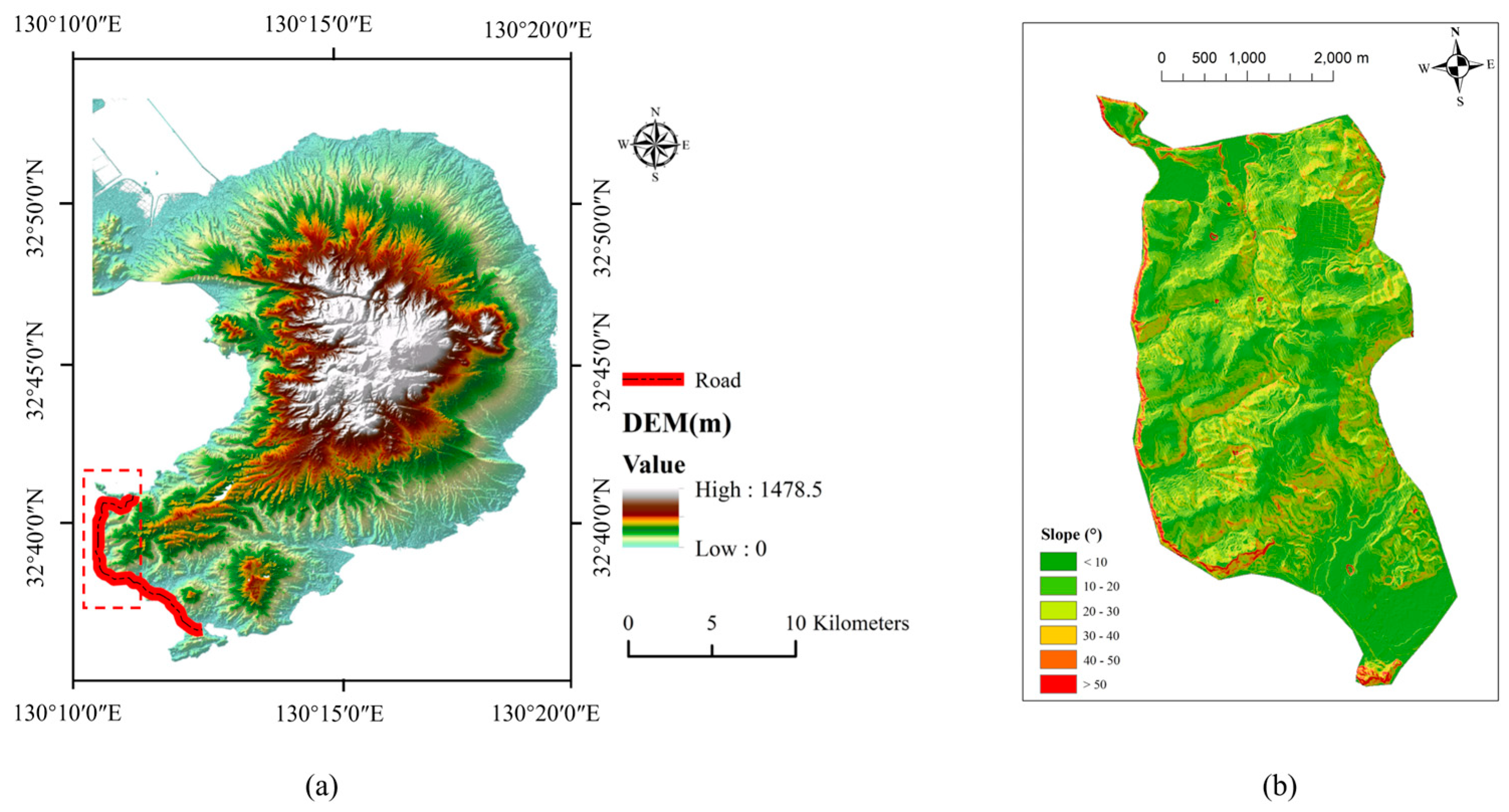
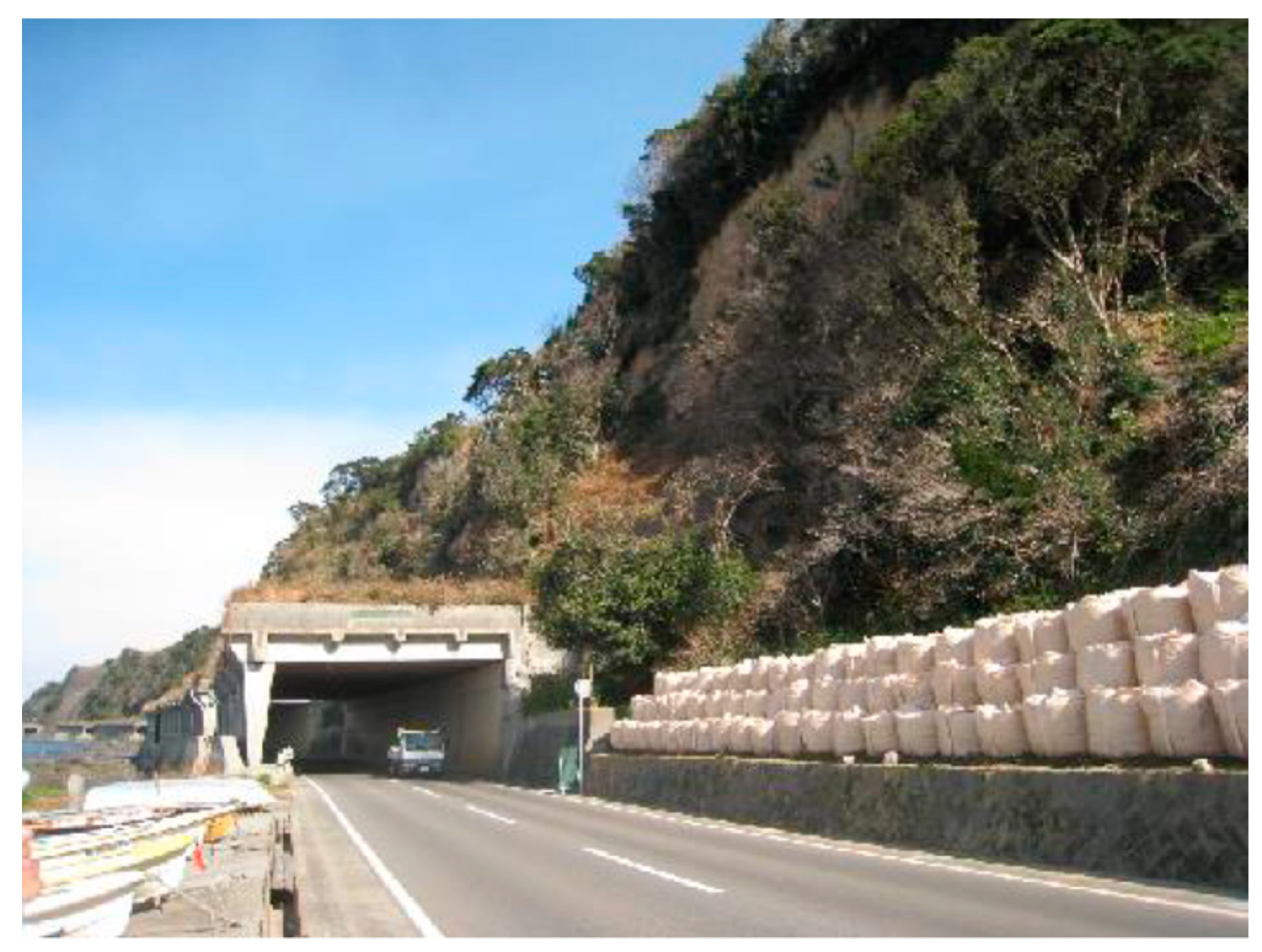
Figure 2a shows the position of the road along the coastline and the digital elevation model (DEM) of the study area. The slope gradient is one of the key factors in assessing slope stability [34]. To roughly evaluate the stability of the slopes along the coastline, a certain area was selected and the slope gradients were extracted based on the grid mapping unit in GIS (Figure 2b). It can be seen that the slope gradient of area along the coastline is primarily around 50°, which falls within a high slope gradient range and requires further stability analysis. Figure 3 shows a photograph of the actual slope, revealing that it is a relatively high and steep slope. The numerical models were built based on the geological data of the actual slope, including the groundwater level, slope height, and slope angle. Only the undulations of the slope surface have been standardized to explore the impact of slope geometry on 3D slope stability. The plane strain assumption in 2D slope stability analysis requires that the slope’s surface appears flat and perpendicular to the analyzed plane. However, both natural and man-made slopes in the real world possess curvature in the third dimension, which leads to significant differences between 3D and 2D calculations. This study aims to investigate how such curvature affects stability by examining the factor of safety (FoS) and potential slip surfaces of 3D slopes with varying curvatures. It is important to note that the curvature considered here is in the third dimension that is perpendicular to the analyzed plane. The curvature within the analyzed plane can be addressed using 2D methods and is not within the scope of this study. In contrast to the research of Zhang et al. [4], this study considers the continuous curvature of slope surfaces, including both convex and concave shapes, in the longitudinal length. The continuous undulation of slope surfaces can also be described in terms of different numbers of turning corners. The stability assessment of the slope along the coastal road directly impacts the design of slope safety measures. Therefore, utilizing the 3D slope stability analysis is crucial for ensuring the safety of the road.

5. Methodology

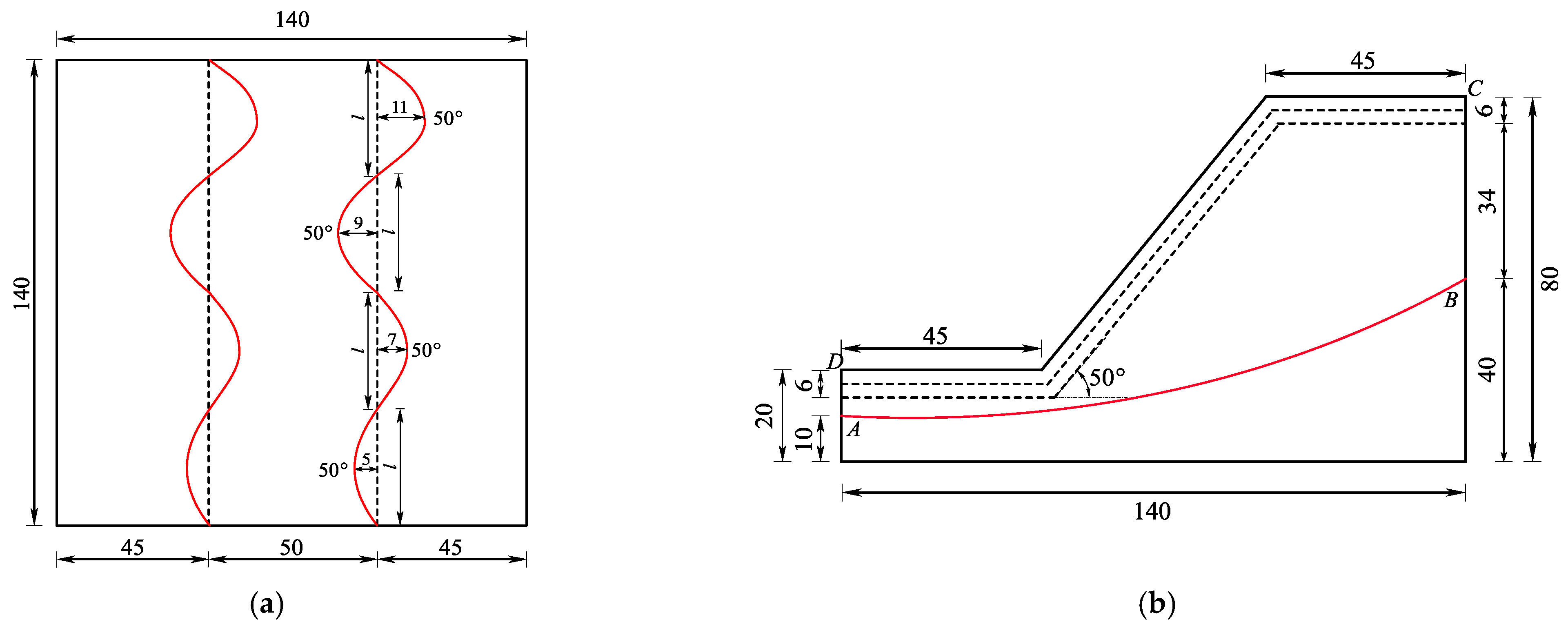
The slope gradient statistics derived from the grid mapping units are not accurate enough to evaluate the regional slope stability, necessitating further division into slope units for a more precise analysis divided based on valley and ridge lines, as shown in Figure 4a. It also shows two different selected sections based on the undulation of the slope within an area of 500 m × 200 m, and the height of slope in two sections is around 80 m. The main difference between the two areas lies in the degree of undulation on the slope surface. The slope surface in Section 1 is relatively smoother compared to Section 2, with the degrees of convexity and concavity being approximately between 5 m and 10 m. The degree of convexity and concavity ranges from approximately 5 m to 20 m in Section 2. The different turning corners are defined as different undulation frequencies of the slope surface in this paper. Various models were established by setting different undulation degrees and frequencies in a certain longitudinal length to explore the influence of complex slope geometries on the 3D stability under heavy rainfall conditions. Depending on the orientation of the slope relative to the direction of the road, slopes were categorized as “parallel to the road” and “oblique to the road” (Figure 4a). It should be noted that the cross-section of slopes intersecting obliquely with the road gradually increases in longitudinal length as shown in Section 1 of Figure 4a. In Section 2 of Figure 4a, it can be observed that the slope orientation is almost parallel to the road, with a significant undulation on the slope surface. The analysis begins by examining the impact of different degrees of surface undulation on the stability of slopes parallel to the road when the slope gradient is set to 50°. Subsequently, the study considers the influence of changes in slope gradient on the stability of 3D slopes based on the same slope models. Additionally, the analysis extends to slopes oblique to the road by investigating the effects of various numbers of turning corners and different degrees of convexity and concavity in a certain longitudinal length on slope stability. Figure 4b shows a typical cross-section of Section 1. The slope consists mainly of two weathered layers with depth of 6 m and bedrock, with the groundwater level indicated in the Figure 4a, b.

5.1. Slopes Parallel to the Road

The first group of models is categorized as an orientation of slopes parallel to the road based on the previous analysis. Four slope examples with different degrees of undulation are analyzed in this section. Figure 5a shows the top view of an example with a continuous convex- and concave-shaped surface geometry, and the dashed line represents the baseline of the slope surface in the figure. The degree of undulation is defined as the distance between the undulation peaks and the baseline. The baseline is divided into four equal parts, with each segment serving as the longitudinal length of the undulation shape. For this slope model, the degree of undulation increases linearly from 5 m to 11 m with an even spacing of 2 m. Figure 5b shows the side view of the slope model, where AB represents the groundwater level and ABCD represents the unsaturated zone above the groundwater with a maximum matric suction of −50 kPa. As pointed out by Rahardjo et al. [34], the length of the slope crest has a minimal impact on slope stability once the slope gradient and height are determined. Therefore, it is reasonable to select this 2D cross-section as the critical cross-section of 3D slope model. The other three sets of models have undulation increments of 0 m, 3 m, and 4 m, respectively. One model has a constant degree of convexity and concavity with 5 m (Figure 6a) and the other has a degree of undulation that increases linearly from 5 m to 14 m with an even spacing of 3 m (Figure 6b). The last one has the degree of undulation that increases linearly from 5 m to 17 m with an even spacing of 4 m. Those four slopes are all inclined at angle of 50° and homogeneous slope material is considered in each weathered layer since this paper primarily analyzes the effects of complex geometries on the 3D slope stability. The slope models were designated as Models P1, P2, P3, and P4 in order of increasing undulation.
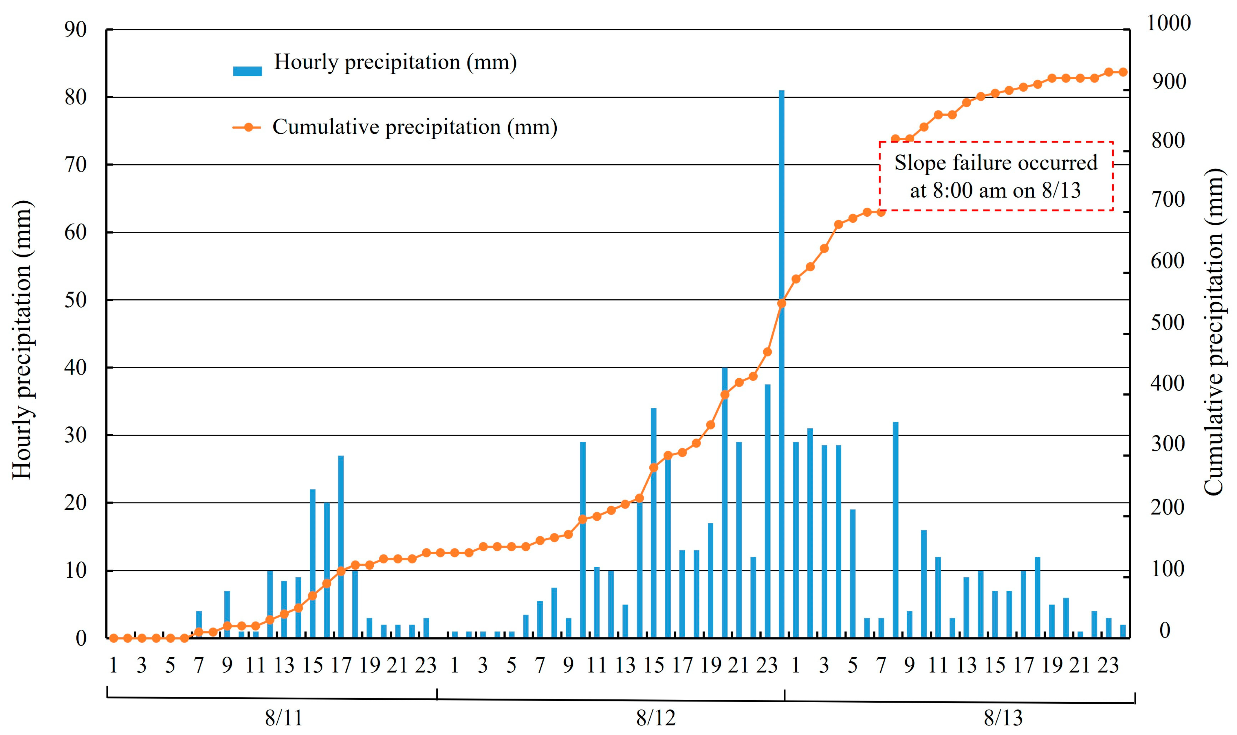
The rainfall data from Unzen County, Nagasaki City, Japan are presented in Figure 7. This rainfall event accumulated to a total of 900 mm in three days (from 11 August to 13 August 2021), which represents an exceptionally high cumulative precipitation. The recorded maximum hourly precipitation reached 81 mm/h, which indicates extremely heavy rainfall in three days. In this numerical simulation, the duration of continuous rainfall was set to 48 h and a sustained rainfall scenario was set at rates of 20 mm/h based on the saturated permeability coefficient of the slope. When the rainfall exceeds this coefficient, the continued increase in rainfall intensity only results in the formation of surface runoff and the rainfall will not infiltrate into the slope. This dynamic rainfall boundary condition can be implemented using the secondary development of FISH functions in FLAC3D, and the pore pressure on the slope surface was set to zero, as shown in Figure 8. This simulation recorded the slope factor of safety at three points for analysis: before rainfall, after 24 h of rainfall, and after 48 h of rainfall.

5.2. Slopes Parallel to the Road with Different Gradients

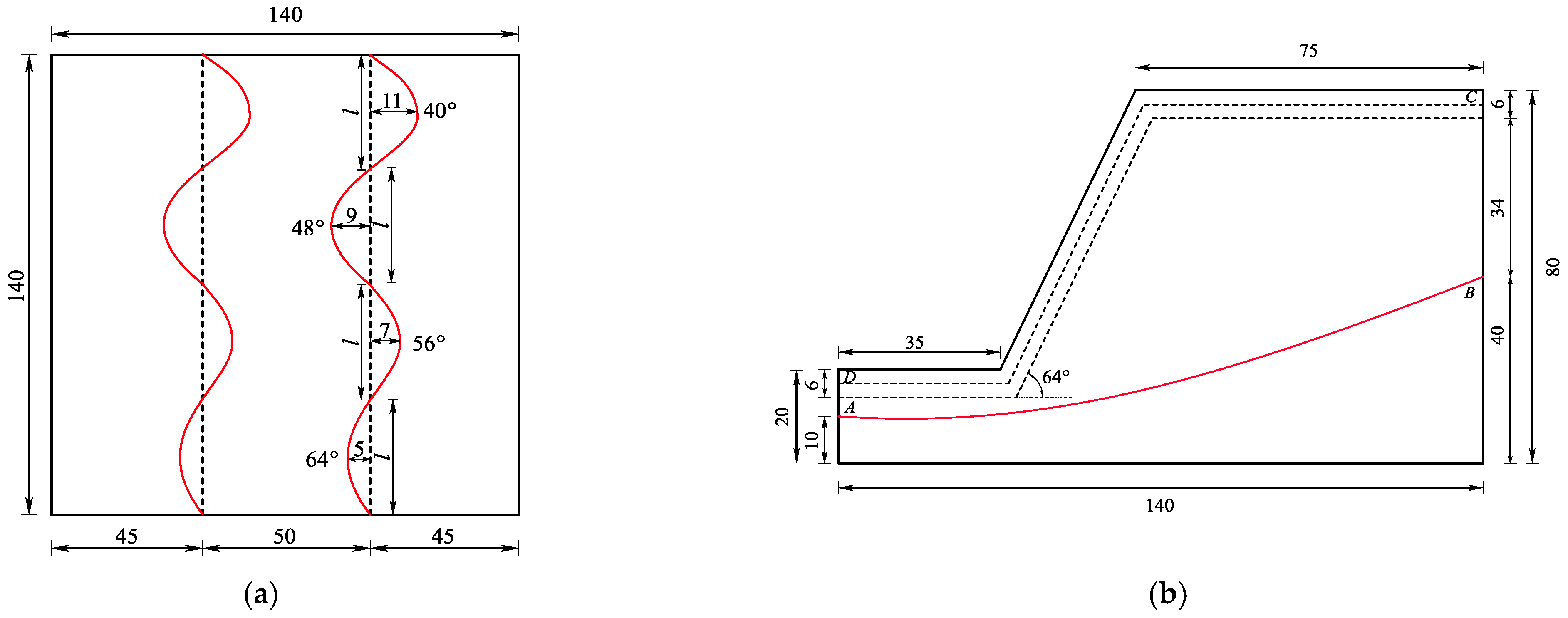
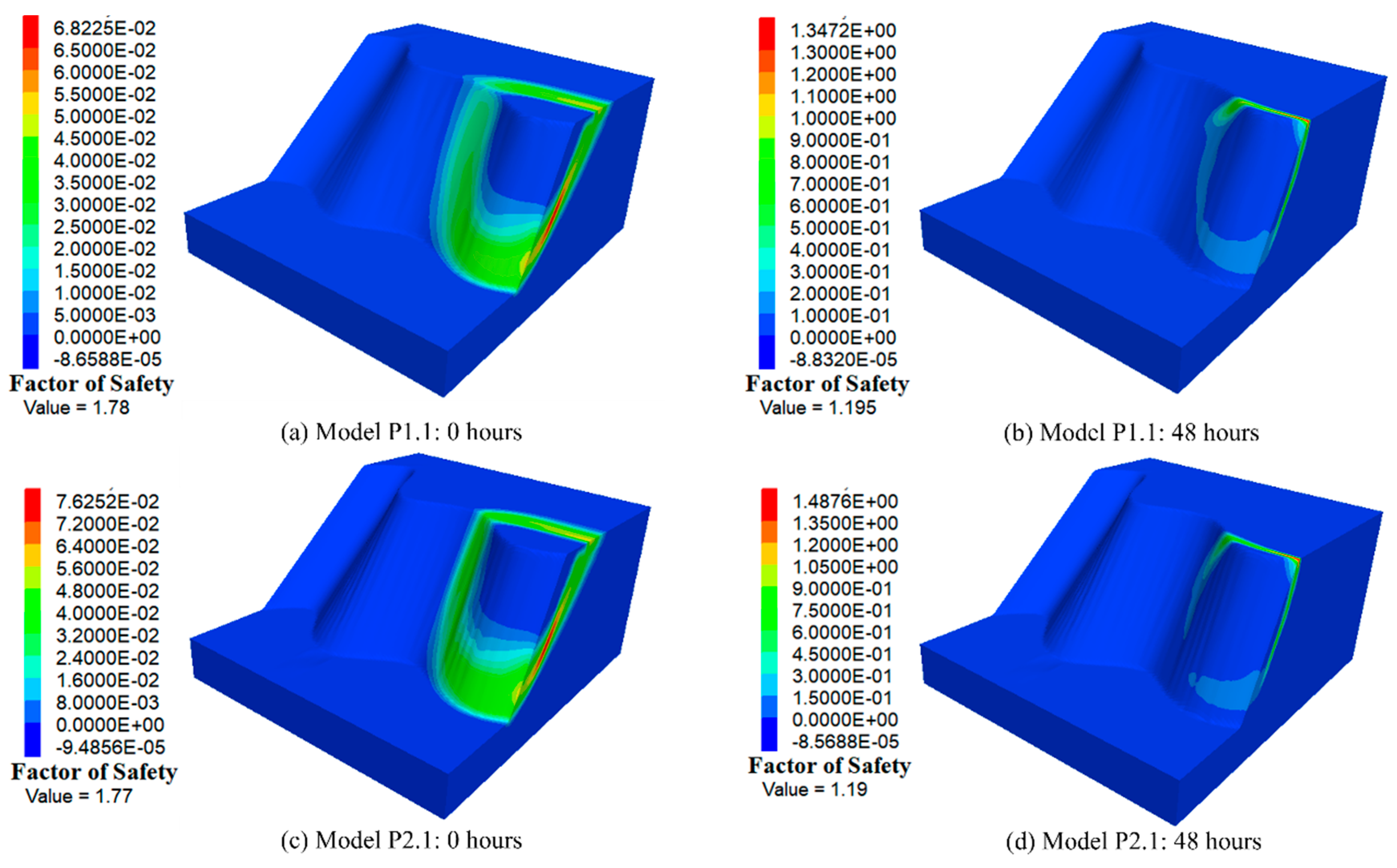
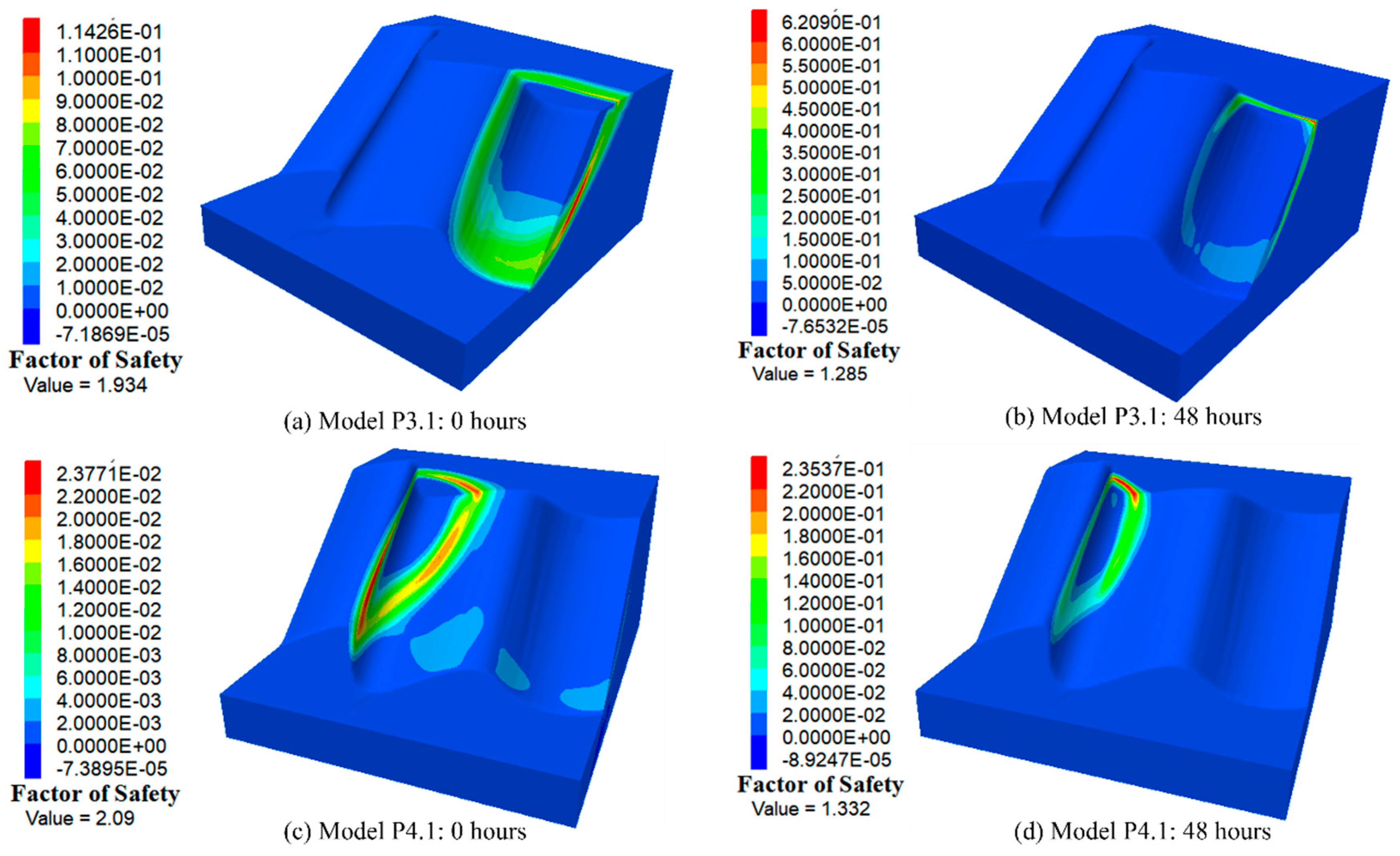
In actual slopes, the slope gradient also varies in addition to the curvature of the slope surface geometry in the longitudinal direction. Therefore, this section discusses the impact of slope gradient changes on the 3D slope stability based on variations in slope surface geometry. Based on the different changes in slope gradient, the second group of models, including Models P1.1, P2.1, P3.1, and P4.1, was established in addition to Models P1, P2, P3, and P4. Figure 9a shows the top view of Model P2.1, where the slope gradient increases from 40° to 64° in increments of 8° for each convex and concave section. For the slope model, the angle refers to the slope inclines at the peak positions of the undulations. The slope gradient is 50° at the inflection points of the slope curvature. For the first convex section, the slope gradient varies incrementally from the slope gradient of 50° to the peak position of 64°, and then the slope gradient decreases from 64° to 50°. For the next concave section, the slope gradient varies incrementally from the slope gradient of 50° to the peak position of 56°, and then the slope gradient decreases from 56° to 50°. Following this procedure, a series of three-dimensional models with different slope gradient variations was established. Figure 9b shows the side view of Model P2.1, and it is also the critical 2D cross-sections of the slope. The slope gradient of Model P1.1 also increases from 40° to 64° in increments of 8° for each convex and concave section (Figure 10a). The slope gradient of Model P3.1 increases from 40° to 58° in increments of 6° for each convex and concave section (Figure 10b). The slope gradient of Model P4.1 increases from 40° to 49° in increments of 3° for each convex and concave section. The purpose of this design is to compare the results with the calculated results from the above section when the slope surface undulation degree is significant but the slope gradient variation is relatively small. This allows us to determine whether the undulation or slope gradient has a greater impact on slope stability. It is worth noting that the slope gradient in Model P4.1 is consistently set below 50°, while the slope gradients in the other slope models vary between greater than and less than 50°. Figure 11 depicts the side views of Models P3.1 and P4.1, which represent the critical 2D cross-sections of these two models.

5.3. Slopes Oblique to the Road

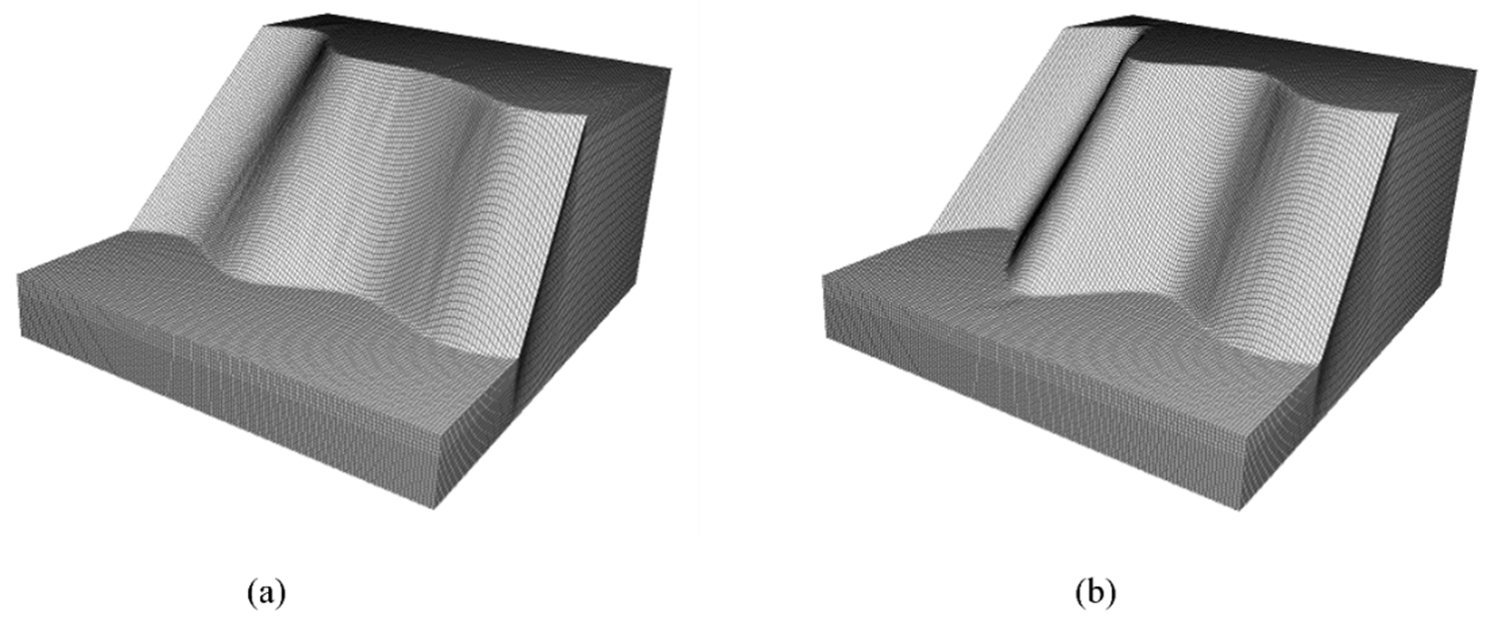
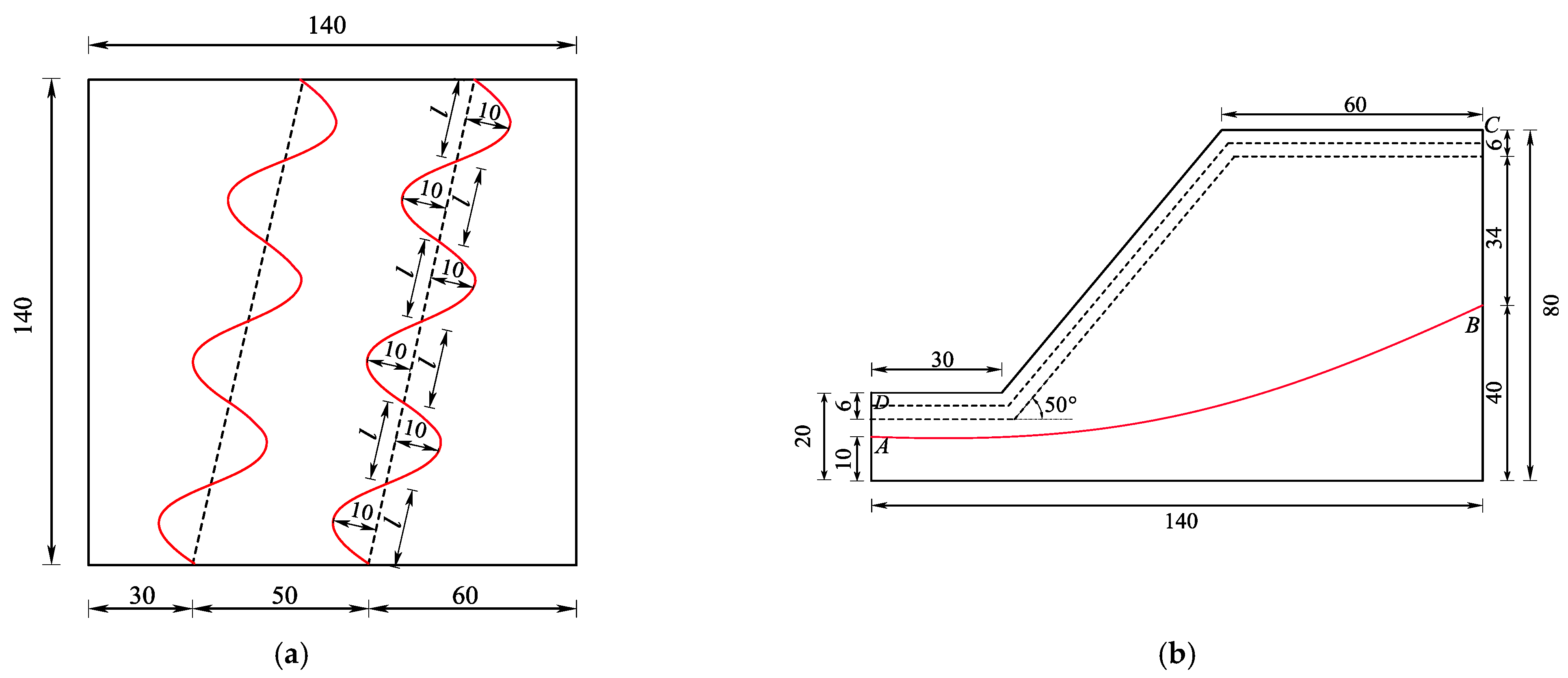
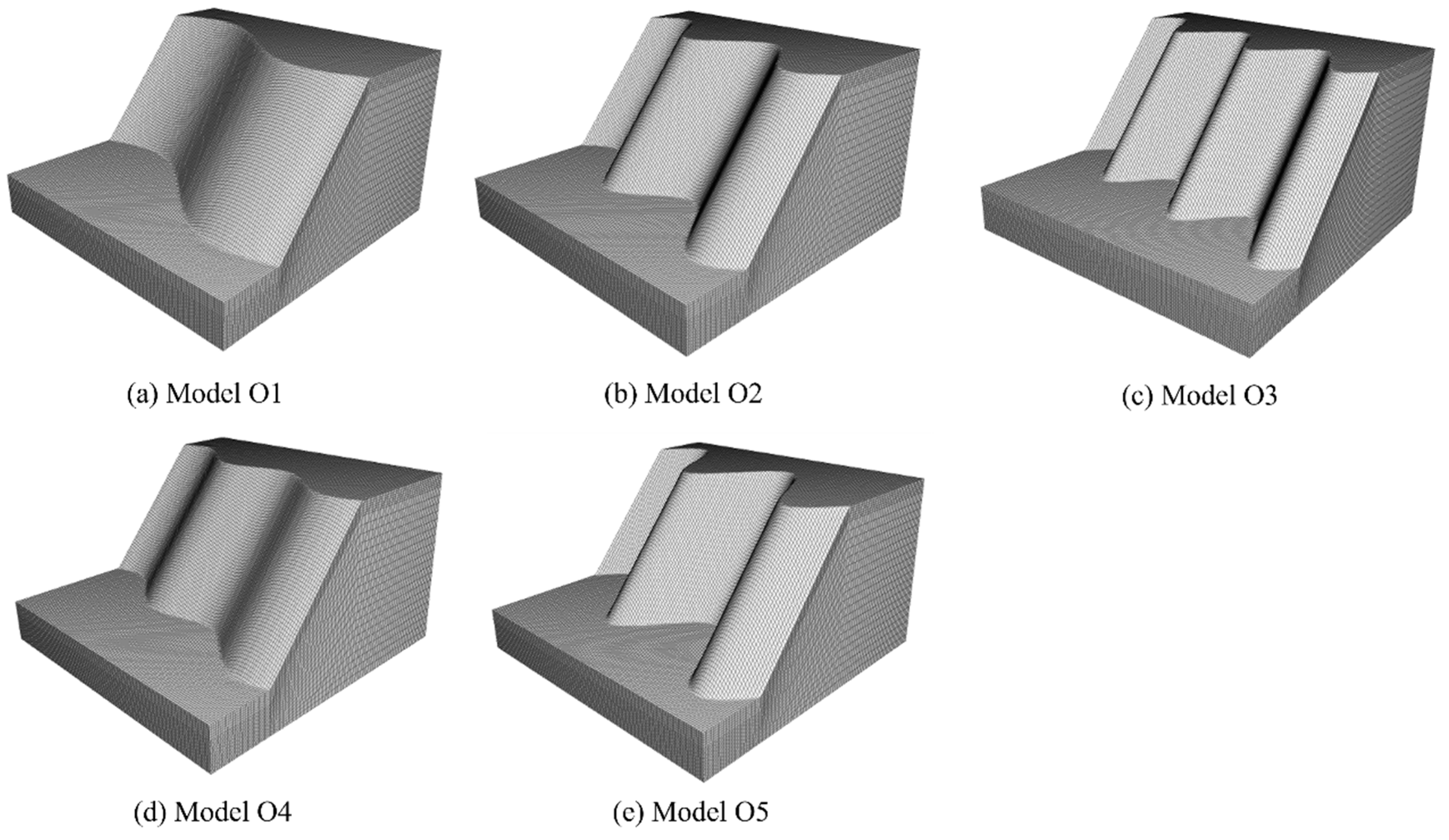
The last two groups of models are categorized as an orientation of slopes oblique to the road direction, based on the previous analysis. Five slope examples with different undulation frequencies and degrees of the surface are analyzed and the slope gradient is maintained at a constant 50° in this section. Figure 12 shows the top and side views of Model O3, and the dashed line represents the baseline of the undulations. The models are divided based on different undulation frequencies into Models O1, O2, and O3, which correspond to undulation frequencies of 2, 4, and 6, respectively. This indicates the number of l segments the baseline is divided into, as shown in Figure 12a. Since the slope gradient and height of the three-dimensional slope models are determined, it is reasonable to select a two-dimensional slope model to represent the critical cross-sections of all these three-dimensional slope models, as shown in Figure 12b. These three models with different undulation frequencies are defined as Group 3. The distance between the peak of the slope undulation and the baseline is defined as the degree of undulation. Two slope models are established, namely, Models O4 and O5, and they represent undulation degrees of 5 m and 15 m, respectively. Both models are set to have the same undulation frequency of 4, as in Model O2. These three models with different undulation degrees are defined as Group 4. All the FDM models of the five 3D slope examples are listed in Figure 13.

6. Results

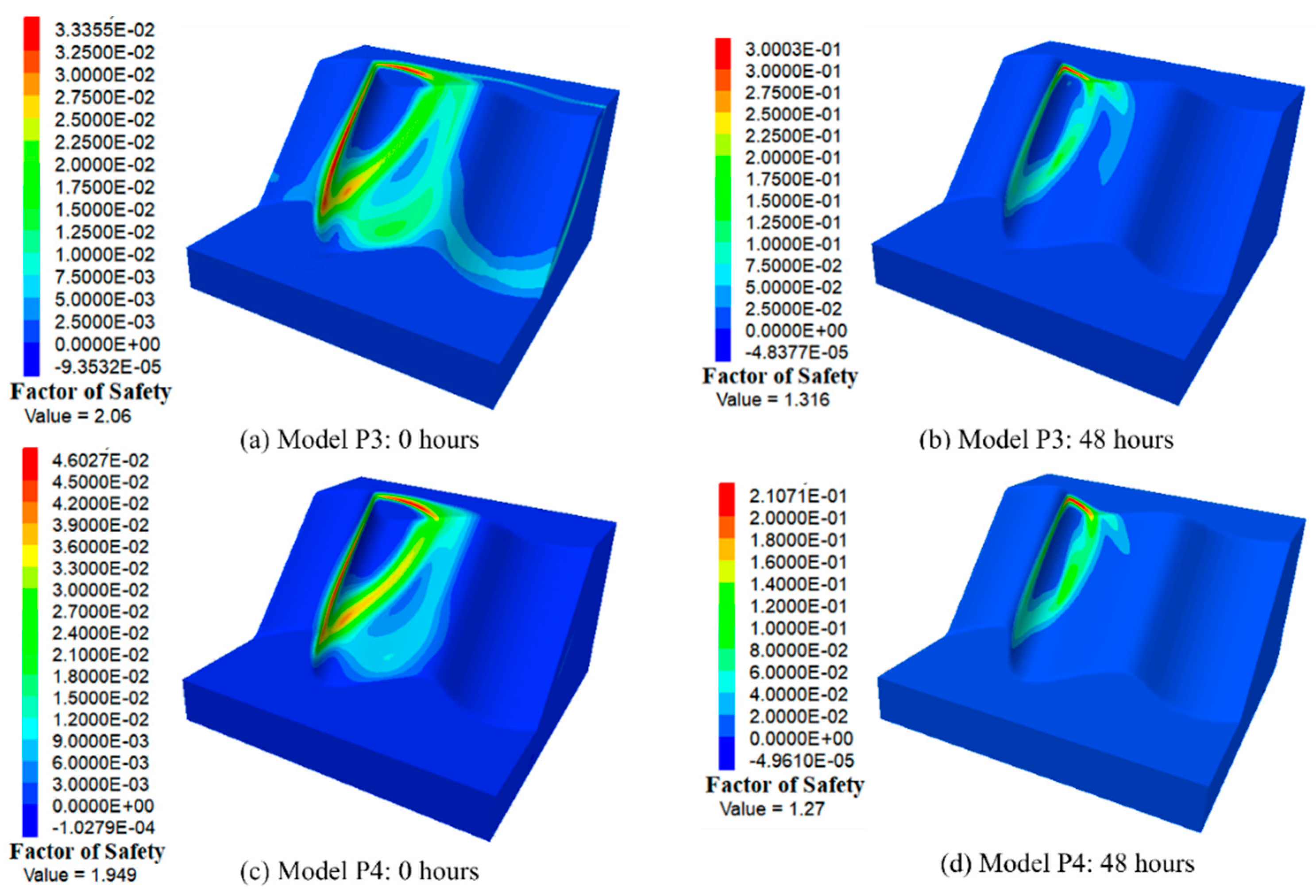
Figure 14 and Figure 15 depict the maximum shear strain and safety factors of the three-dimensional slopes in Group 1 before rainfall and after 48 h of rainfall, respectively. When the undulation amplitude is 5 m for each convex- and concave-shaped surface, this means that there is no increment in the undulation amplitude (the increment distance is 0 m). It can be observed that in Model 1, both initially and after 48 h of rainfall, the potential slip surfaces tend to involve the entire slope (Figure 14a,b). However, when there is variability in the undulation amplitude, such as an increment distance of 2 m, after 48 h of rainfall, the maximum shear strain areas of the slope begin to concentrate in the most prominent regions of the slope, as shown in Figure 14d. When the undulation amplitude continues to increase to 3 m and 4 m, Figure 15a,c reveals that initially, the potential slip surfaces of the slope are located in the most prominent areas of the slope’s surface. The potential slip surfaces begin to move towards to the most concave areas of the slope surface as the rainfall progresses. It can be observed in Figure 15b,d that both initially and after 48 h of rainfall, the potential slip surfaces of the slope are concentrated between the most convex peaks and concave peaks of the slope. It indicates that the most hazardous area of the slope is in the regions with the highest degrees of convexity and concavity after 48 h of rainfall. This differs from the hazardous areas of the slope in its initial state. Figure 16 and Figure 17 depict the maximum shear strain and safety factors of the three-dimensional slopes in Group 2 before rainfall and after 48 h of rainfall, respectively. When changes in the slope gradient are considered in slope geometry, it is observed that the area of maximum shear strain concentrates in the region with the steepest gradient before and after 48 h of rainfall if the slope gradient exceeds 50° (Figure 16). However, when the undulation degree is maximal but the range of slope gradients remains below 50° in Model 4.1, the potential sliding surface of the slope remains situated in the most protruding area of the slope rather than in the area with the steepest gradient (49°), as illustrated in Figure 17c, d. This indicates that the variation in slope gradient has a greater impact on slope stability compared to changes in the undulation of the slope surface. Initially, the potential slip surfaces of the 3D slopes with undulation amplitude increments of 0 m and 2 m tend to experience overall failure. For undulation amplitude increments of 2 m, 3 m, and 4 m, the potential slip surfaces of the slope are located in the most prominent areas. After 48 h of rainfall, the potential slip surfaces of the 3D slopes are also located in the most prominent positions.
Table 3 summarizes the stability of 3D slopes with different undulation degrees and slope gradients for Groups 1 and 2. When the undulation frequency is four and the slope gradient is 50°, the larger the increment distance of the undulation amplitude, the smaller the slope’s factor of safety (FoS) after rainfall for 24 h and 48 h. The FoS of the 2D cross-section is only lower than the safety factors of the 3D slopes with undulation amplitude increments of 0 m and 2 m, indicating that when the slope undulation amplitude increment is significant (e.g., 4 m), the safety factor of the 2D critical cross-section cannot represent the safety factor of the 3D model. It is illustrated that the 2D calculations are not necessarily more conservative than the 3D analysis when the slope geometry is complex. Therefore, it is necessary to calculate the safety factor of the 3D slope in this scenario. When slope gradient variations are incorporated, the FoS for the 2D critical cross-section with the steepest gradient is lower than that of the 3D slope, making the 2D calculation results more conservative. However, it is challenging to identify the 2D cross-section with the steepest gradient over a given longitudinal range in practical engineering. If a cross-section with 50° slope gradient is selected as the critical section, it can result in a FoS of 3D slopes that is lower than the 2D critical section, leading to a misjudgment of slope stability. On the other hand, selecting the steepest 2D cross-section (64°) as the critical cross-section may result in an overly conservative slope design. Table 3 presents the difference in the factors of safety (DF) between a 2D and a 3D slope stability analysis ((Fs3-D − Fs2-D)/Fs2-D, or ΔFs/Fs2-D).
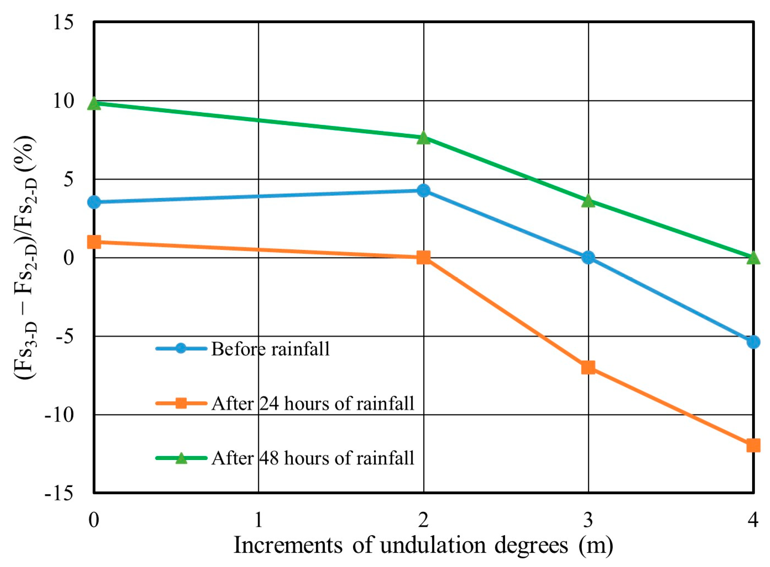
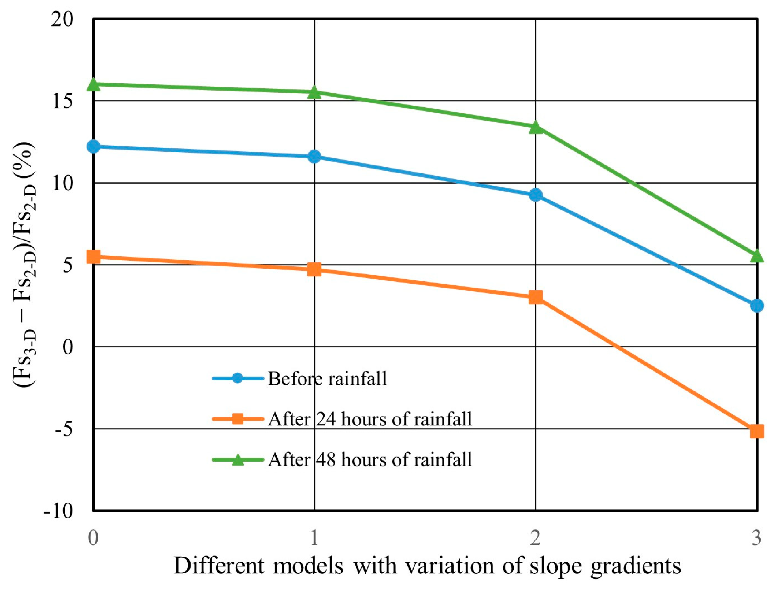
Figure 18 indicates that as the undulation degree of the slope surface increases, the safety factor of the three-dimensional slope decreases under the same rainfall duration. However, the difference in safety factors (DF) between 2D and 3D slopes remains positive when the undulation increments are 0 m, 2 m, and 3 m, indicating that the 2D analysis is still more conservative in these cases. When the undulation increment reaches 4 m, the differences in FoS before rainfall and 24 h of rainfall are −5.39% and −11.97%, respectively. In this case, the 3D calculation results are lower than the 2D results, demonstrating that when the slope surface undulation reaches a certain level, the 2D analysis is not more conservative than the 3D analysis. Similarly, Figure 19 clearly shows that although the slope gradient changes, the FoS of the 3D slope decreases gradually as the degree of undulation increases after 24 h and 48 h of rainfall. However, since the most critical 2D cross-section with the maximum slope gradient was considered, the differences between 2D and 3D safety factors remain mostly positive. It shows that the 2D safety factors are more conservative than the 3D ones. This aligns with the traditional 2D safety factor calculations based on the plane strain assumption, which assumes an infinite length in the longitudinal direction. The FoS of the 2D analysis is typically lower than that of the 3D analysis. This is because the entire slope is considered to have a gradient of 64° in the extended 2D model, which is evidently less safe than a 3D slope with gradients increasing from 40° to 64°. Taking Model P1.1 as an example, the differences in safety factors between the 2D and 3D slopes before rainfall and 48 h after rainfall are 12.23% and 16.02%, respectively. Similarly, the differences are 11.60% and 15.53% for Model P2.1, respectively. Although selecting the 2D representative cross-section based on the maximum slope gradients results in safer outcomes, it also leads to inefficiencies in slope safety design. It is obvious that conducting the 3D slope stability analysis allows for a more rational and efficient slope safety design.
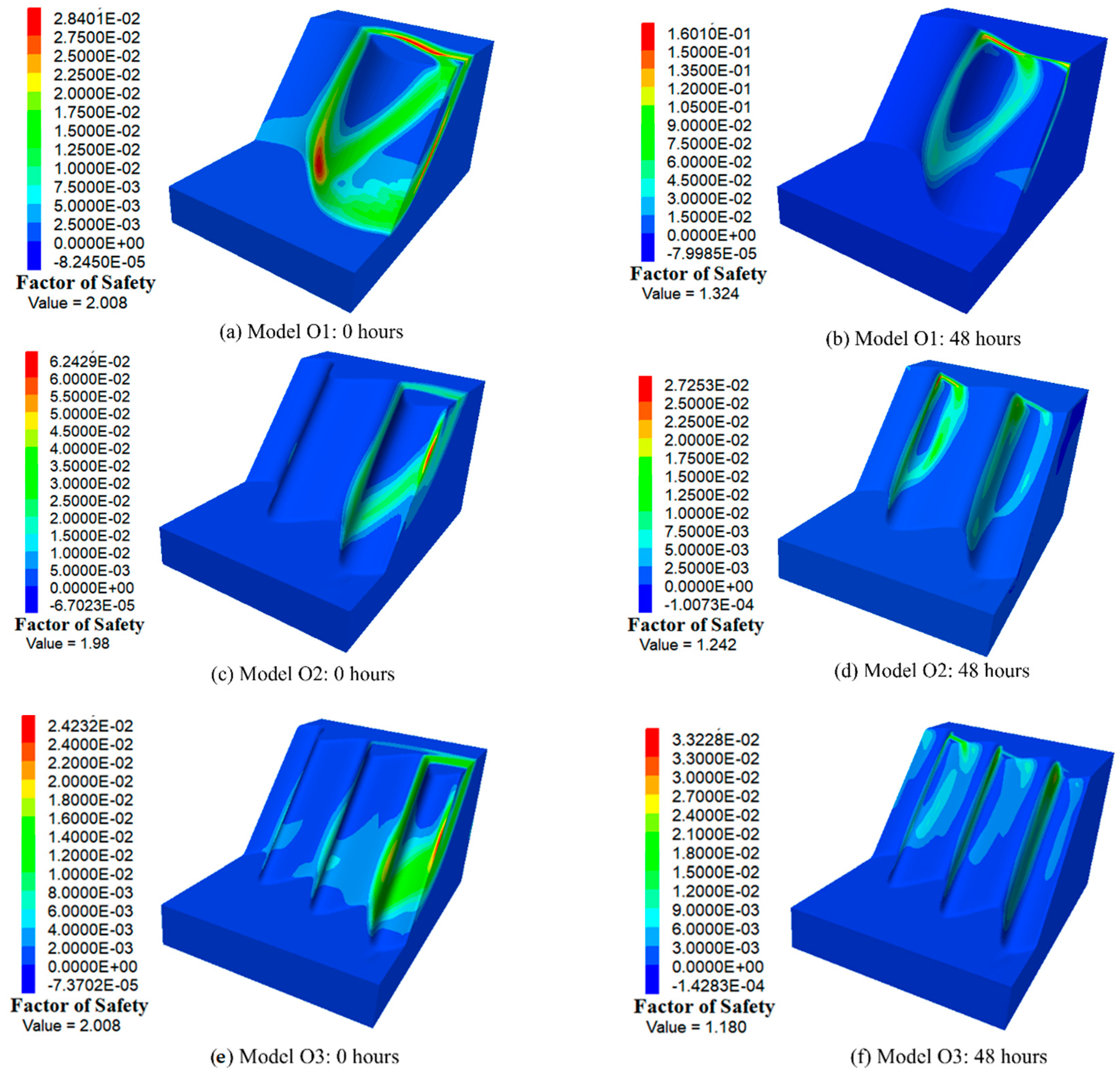
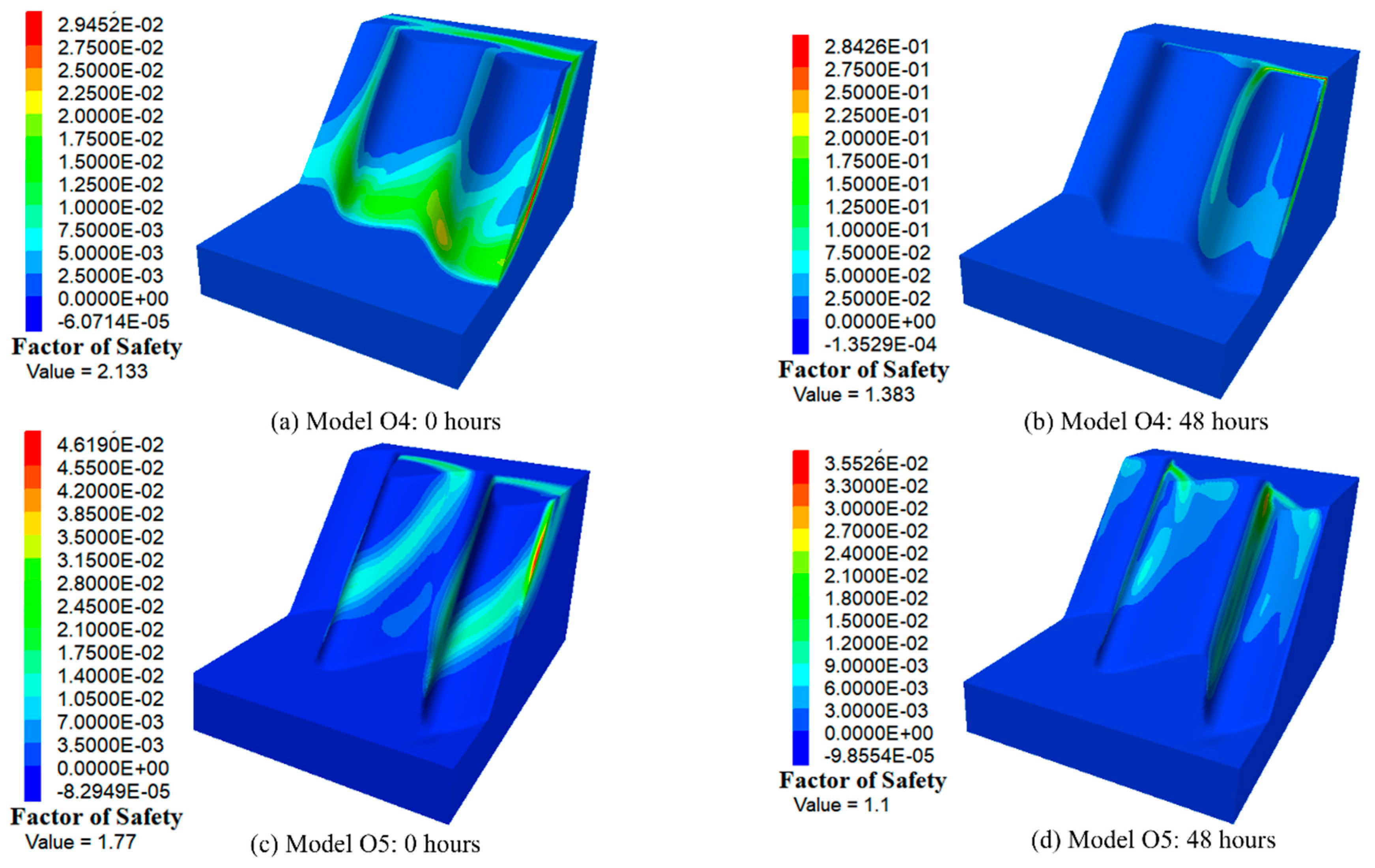
Figure 20 depicts the maximum shear strain and safety factors of the three-dimensional slopes in Group 3 before rainfall and after 48 h of rainfall, respectively. When the undulation amplitude is 10 m, the post-rain FOS of the slope decreases with increasing undulation frequency. Overall, the FOS of the 2D cross-section is greater than that of the 3D slope, indicating that the safety coefficient of the 2D critical section cannot fully represent the safety of the 3D model when the slope undulation is large, thus requiring the calculation of the safety coefficient of the 3D slope. After 48 h of rainfall, the potential sliding surface of the 3D slope is in the most prominent area of the slope. Figure 21 depicts the maximum shear strain and safety factors of the three-dimensional slopes in Group 4 before rainfall and after 48 h of rainfall, respectively. When the undulation frequency is four, the larger the undulation amplitude, the smaller the FOS of the slope after rainfall. The FOS of the 2D cross-section is only less than that of the 3D slope when the undulation amplitude is 5 m. This indicates that when the undulation amplitude of the slope is large, the safety coefficient of the 2D critical section cannot represent the safety of the 3D model, and the safety coefficient of the 3D slope must be calculated. After 48 h of rainfall, the potential sliding surface of the 3D slope is in the most prominent area of the slope. Table 4 summarizes the stability of 3D slopes with different undulation degrees and frequencies.
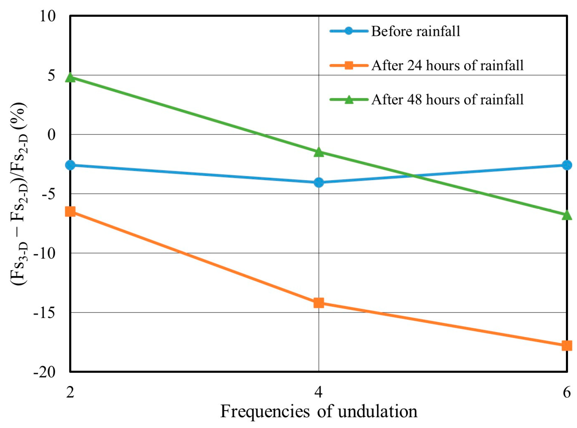
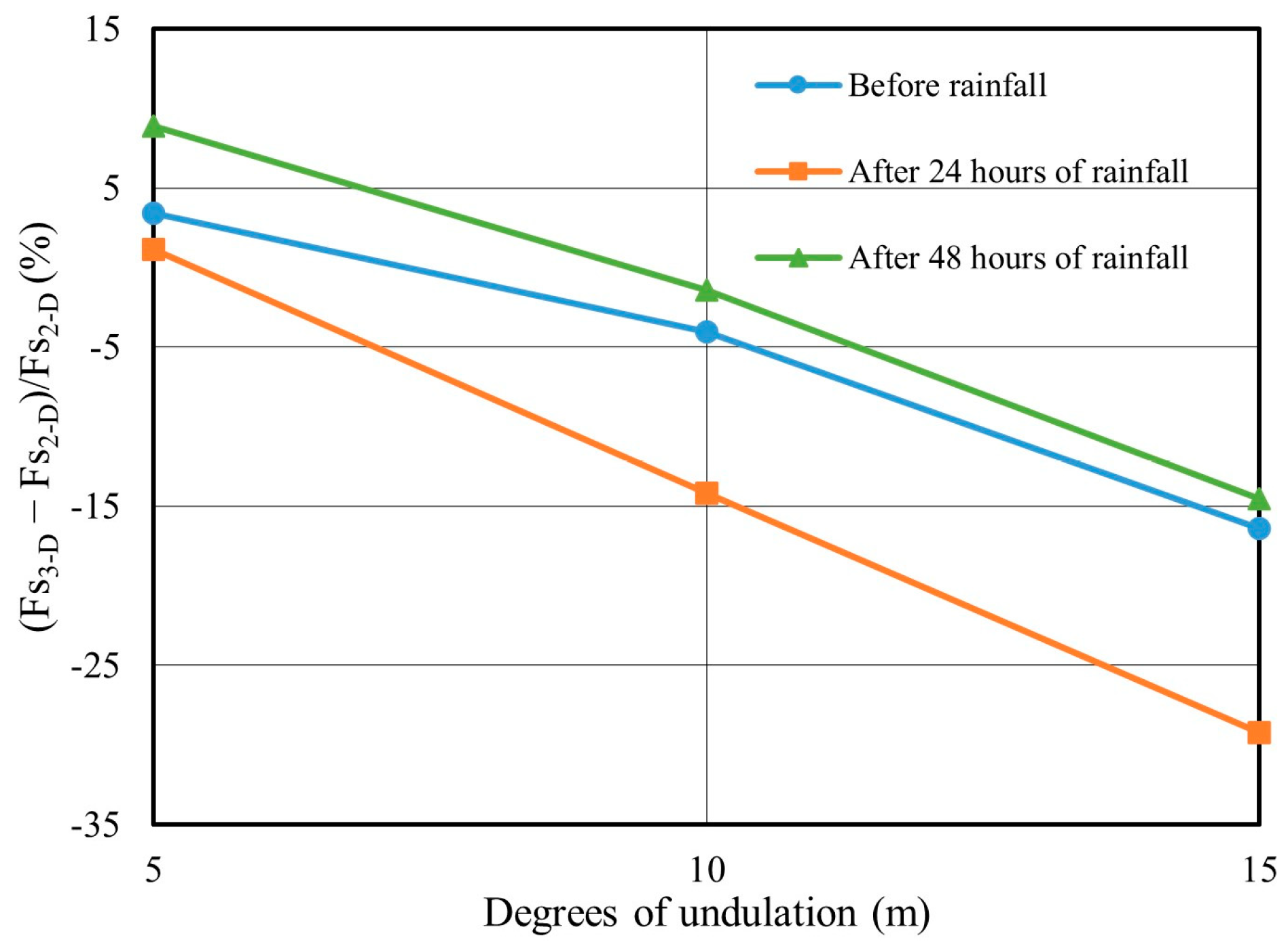
Table 4 summarizes the stability of 3D slopes with different undulation degrees and frequencies. The results from Group 4 illustrate that the FoS decreases as the undulation frequency increases when the undulation magnitude is constant (10 m). For undulation frequencies of four and six, the FoS for the 3D slope is lower than that for the selected 2D critical cross-section. This also demonstrates that the 2D analysis is not necessarily more conservative than 3D calculations in cases of complex slope surface geometries. When the undulation frequency is constant and the undulation magnitudes are 10 m and 15 m, the FoS for the 3D slope is lower than that for the 2D critical cross-section. It is clear that the greater the undulation magnitude, the more pronounced the difference between 2D and 3D analyses. Figure 22 shows that the difference in safety factors for the 3D slopes caused by different undulation frequencies is minimal before rainfall when the undulation degree is 10 m. However, the differences between the 2D and 3D slope safety factors become significant after 24 h and 48 h of rainfall. Particularly, the safety factor differences between the 3D slopes with undulation frequencies of four and six and the 2D critical section reach −14.18% and −17.78% after 24 h of rainfall, respectively. Overall, the safety factors for the 3D slope analysis with different undulation frequencies are generally lower than those for 2D slopes. Although these differences decrease after 48 h of rainfall, the difference between 2D and 3D safety factors with an undulation frequency of six still reaches −6.78%. Figure 23 shows that the safety factor for the 3D slope is greater than that for the 2D critical section when the undulation degree is small (e.g., 5 m). However, the differences between 2D and 3D values become significant when the undulation degree reaches 15 m. The differences in safety factors before rainfall and after 24 h and 48 h of rainfall are −16.4%, −29.21%, and −14.54%, respectively. This demonstrates that the traditional method of selecting a 2D critical section cannot replace the analysis of 3D slope stability when the slope surface undulation degree is large, as it leads to significant misjudgments for the slope design.

7. Conclusions

To investigate the differences in slope stability caused by varying spatial dimensions after short-term heavy rainfall when the slope geometries are complex, four groups of models were designed for numerical simulation in this study. The first group examines different undulation increments of the slope surface with the same undulation frequency. The second group adds varying slope gradients of different concave and convex sections based on the first group. The results from these two groups indicate that a greater undulation degree leads to lower slope stability after rainfall, regardless of whether the slope gradient remains constant or varies. When the undulation increment of the slope surface is 4 m within a certain longitudinal length, the safety factors of the 3D slope before rainfall, 24 h after rainfall, and 48 h after rainfall are all lower than those of the selected 2D critical section. This indicates that the 2D analysis is not necessarily more conservative than the 3D analysis when the geometric undulation of a 3D slope surface reaches a certain level. When the slope gradient variation is large (40° to 64°), selecting the 2D critical section with the maximum slope gradient results in overly conservative calculations, potentially leading to excessive and wasteful slope safety designs. Therefore, conducting an actual 3D slope stability analysis is necessary for rational and efficient slope protection design.
The third group of slope models considers a fixed undulation degree (10 m) with varying undulation frequencies within a certain longitudinal length. The results show that the higher the undulation frequency of the 3D slope surface, the lower the slope safety factor after short-term heavy rainfall. Even with an undulation frequency of only two, the safety factors of the 3D slope before and 24 h after rainfall are still lower than the 2D calculation results. The fourth group of models examines a fixed undulation frequency with varying undulation degrees within a certain longitudinal length. The results show that the greater the undulation degree, the lower the 3D slope safety factor after short-term heavy rainfall. It is worth noting that the difference in safety factors between the 3D and 2D slopes becomes more pronounced when the undulation degree exceeds 10 m. This demonstrates that the complex geometric surfaces of 3D slopes can lead to significant differences in calculation results compared to the traditional method of selecting the 2D critical section of the slope. Therefore, performing an actual 3D slope stability analysis is crucial when the slope surface geometry is complex since the impact of different spatial dimensions on slope stability is highly significant. It is highly recommended that geotechnical engineers conduct both 2D and 3D analyses to provide sufficient confidence in designs.

Author Contributions

Conceptualization, X.L. and Y.J.; methodology, X.L. and Y.J.; writing—original draft preparation, X.L.; writing—review and editing, Y.J.; supervision, Y.J. and S.S. All authors have read and agreed to the published version of the manuscript.

Funding

This research received no external funding.

Data Availability Statement

The data presented in this study are available on request from the corresponding author.

Acknowledgments

This study was supported by the “Project for Fostering of Proficient Researchers for the Establishment of the Research Center for Green Science”.

Conflicts of Interest

The authors declare no conflicts of interest.

References

  1. Sheikh, M.R.; Nakata, Y.; Shitano, M.; Kaneko, M. Rainfall-Induced Unstable Slope Monitoring and Early Warning through Tilt Sensors. Soils Found. 2021, 61, 1033–1053. [Google Scholar] [CrossRef]
  2. Chen, H.; Qin, S.; Xue, L.; Xu, C. Why the Xintan Landslide Was Not Triggered by the Heaviest Historical Rainfall: Mechanism and Review. Eng. Geol. 2021, 294, 106379. [Google Scholar] [CrossRef]
  3. Cho, M.T.T.; Chueasamat, A.; Hori, T.; Saito, H.; Kohgo, Y. Effectiveness of Filter Gabions against Slope Failure Due to Heavy Rainfall. Soils Found. 2021, 61, 480–495. [Google Scholar] [CrossRef]
  4. Zhang, Y.; Chen, G.; Zheng, L.; Li, Y.; Zhuang, X. Effects of Geometries on Three-Dimensional Slope Stability. Can. Geotech. J. 2013, 50, 233–249. [Google Scholar] [CrossRef]
  5. Jaboyedoff, M.; Carrea, D.; Derron, M.-H.; Oppikofer, T.; Penna, I.M.; Rudaz, B. A Review of Methods Used to Estimate Initial Landslide Failure Surface Depths and Volumes. Eng. Geol. 2020, 267, 105478. [Google Scholar] [CrossRef]
  6. Azizian, A.; Popescu, R. Three-Dimensional Seismic Analysis of Submarine Slopes. Soil. Dyn. Earthq. Eng. 2006, 26, 870–887. [Google Scholar] [CrossRef]
  7. Leong, E.C.; Rahardjo, H. Two and Three-Dimensional Slope Stability Reanalyses of Bukit Batok Slope. Comput. Geotech. 2012, 42, 81–88. [Google Scholar] [CrossRef]
  8. Wines, D. A Comparison of Slope Stability Analyses in Two and Three Dimensions. J. S. Afr. Inst. Min. Metall. 2016, 116, 399–406. [Google Scholar] [CrossRef]
  9. Griffiths, D.V.; Marquez, R.M. Three-Dimensional Slope Stability Analysis by Elasto-Plastic Finite Elements. Géotechnique 2007, 57, 537–546. [Google Scholar] [CrossRef]
  10. Wei, W.B.; Cheng, Y.M.; Li, L. Three-Dimensional Slope Failure Analysis by the Strength Reduction and Limit Equilibrium Methods. Comput. Geotech. 2009, 36, 70–80. [Google Scholar] [CrossRef]
  11. Zhang, L.L.; Fredlund, M.D.; Fredlund, D.G.; Lu, H.; Wilson, G.W. The Influence of the Unsaturated Soil Zone on 2-D and 3-D Slope Stability Analyses. Eng. Geol. 2015, 193, 374–383. [Google Scholar] [CrossRef]
  12. Zhou, Y.; Qi, S.-C.; Fan, G.; Chen, M.-L.; Zhou, J.-W. Topographic Effects on Three-Dimensional Slope Stability for Fluctuating Water Conditions Using Numerical Analysis. Water 2020, 12, 615. [Google Scholar] [CrossRef]
  13. Yeh, P.-T.; Lee, K.Z.-Z.; Chang, K.-T. 3D Effects of Permeability and Strength Anisotropy on the Stability of Weakly Cemented Rock Slopes Subjected to Rainfall Infiltration. Eng. Geol. 2020, 266, 105459. [Google Scholar] [CrossRef]
  14. Sabzevari, T.; Noroozpour, S. Effects of Hillslope Geometry on Surface and Subsurface Flows. Hydrogeol. J. 2014, 22, 1593–1604. [Google Scholar] [CrossRef]
  15. Talebi, A.; Troch, P.A.; Uijlenhoet, R. A Steady-state Analytical Slope Stability Model for Complex Hillslopes. Hydrol. Process. 2008, 22, 546–553. [Google Scholar] [CrossRef]
  16. Wang, J.; Chen, L. The Effect of Hillslope Geometry on Hortonian Rainfall-Infiltration-Runoff Processes. J. Hydrol. 2021, 594, 125962. [Google Scholar] [CrossRef]
  17. Xu, J.; Zhao, X.; Li, P.; Zhang, M. Stability of a 3D Unsaturated Vertical Cut Slope Subjected to Variable Rainfall Infiltration. Comput. Geotech. 2021, 134, 104110. [Google Scholar] [CrossRef]
  18. Zhang, L.; Gong, W.; Li, X.; Tan, X.; Zhao, C.; Wang, L. A Comparison Study between 2D and 3D Slope Stability Analyses Considering Spatial Soil Variability. J. Zhejiang Univ. Sci. A 2022, 23, 208–224. [Google Scholar] [CrossRef]
  19. Tozato, K.; Dolojan, N.L.J.; Touge, Y.; Kure, S.; Moriguchi, S.; Kawagoe, S.; Kazama, S.; Terada, K. Limit Equilibrium Method-Based 3D Slope Stability Analysis for Wide Area Considering Influence of Rainfall. Eng. Geol. 2022, 308, 106808. [Google Scholar] [CrossRef]
  20. Zheng, H. A Three-dimensional Rigorous Method for Stability Analysis of Landslides. Eng. Geol. 2012, 145–146, 30–40. [Google Scholar] [CrossRef]
  21. Li, A.J.; Merifield, R.S.; Lyamin, A.V. Three-Dimensional Stability Charts for Slopes Based on Limit Analysis Methods. Can. Geotech. J. 2010, 47, 1316–1334. [Google Scholar] [CrossRef]
  22. Michalowski, R.L. Limit Analysis and Stability Charts for 3D Slope Failures. J. Geotech. Geoenviron. Eng. 2010, 136, 583–593. [Google Scholar] [CrossRef]
  23. Nian, T.-K.; Huang, R.-Q.; Wan, S.-S.; Chen, G.-Q. Three-Dimensional Strength-Reduction Finite Element Analysis of Slopes: Geometric Effects. Can. Geotech. J. 2012, 49, 574–588. [Google Scholar] [CrossRef]
  24. Ugai, K.; Leshchinsky, D. Three-Dimensional Limit Equilibrium and Finite Element Analyses: A Comparison of Results. Soils Found. 1995, 35, 1–7. [Google Scholar] [CrossRef] [PubMed]
  25. Zienkiewicz, O.C.; Humpheson, C.; Lewis, R.W. Associated and Non-Associated Visco-Plasticity and Plasticity in Soil Mechanics. Géotechnique 1975, 25, 671–689. [Google Scholar] [CrossRef]
  26. Sun, C.; Chai, J.; Xu, Z.; Qin, Y. 3D Stability Charts for Convex and Concave Slopes in Plan View with Homogeneous Soil Based on the Strength-Reduction Method. Int. J. Geomech. 2017, 17, 06016034. [Google Scholar] [CrossRef]
  27. Ietto, F.; Perri, F.; Cella, F. Weathering Characterization for Landslides Modeling in Granitoid Rock Masses of the Capo Vaticano Promontory (Calabria, Italy). Landslides 2018, 15, 43–62. [Google Scholar] [CrossRef]
  28. Perri, F.; Ietto, F.; Le Pera, E.; Apollaro, C. Weathering Processes Affecting Granitoid Profiles of Capo Vaticano (Calabria, Southern Italy) Based on Petrographic, Mineralogic and Reaction Path Modelling Approaches. Geol. J. 2016, 51, 368–386. [Google Scholar] [CrossRef]
  29. van Genuchten, M.T. A Closed-Form Equation for Predicting the Hydraulic Conductivity of Unsaturated Soils. Soil. Sci. Soc. Am. J. 1980, 44, 892–898. [Google Scholar] [CrossRef]
  30. Pan, Y.; Wu, G.; Zhao, Z.; He, L. Analysis of Rock Slope Stability under Rainfall Conditions Considering the Water-Induced Weakening of Rock. Comput. Geotech. 2020, 128, 103806. [Google Scholar] [CrossRef]
  31. Dawson, E.M.; Roth, W.H.; Drescher, A. Slope Stability Analysis by Strength Reduction. Géotechnique 1999, 49, 835–840. [Google Scholar] [CrossRef]
  32. Shen, H.; Klapperich, H.; Abbas, S.M.; Ibrahim, A. Slope Stability Analysis Based on the Integration of GIS and Numerical Simulation. Autom. Constr. 2012, 26, 46–53. [Google Scholar] [CrossRef]
  33. Xu, Y.; Li, J.; Fan, H.; Chen, L.; Zhao, Y.; Li, L. Stability Analysis of Clastic Rock Slope with Mudstone Interlayer Under Rainfall Infiltration. Geotech. Geol. Eng. 2017, 35, 1871–1883. [Google Scholar] [CrossRef]
  34. Rahardjo, H.; Ong, T.H.; Rezaur, R.B.; Leong, E.C. Factors Controlling Instability of Homogeneous Soil Slopes under Rainfall. J. Geotech. Geoenviron. Eng. 2007, 133, 1532–1543. [Google Scholar] [CrossRef]
Figure 1. The distribution of pore pressure in the slope before rainfall.
Geohazards 05 00037 g001
Figure 2. (a) The position of the city road and the study area is within the red dashed lines. (b) The slope gradient statistics are derived from the grid mapping units, and the slope gradient is mainly around 50°.
Geohazards 05 00037 g002
Figure 3. A photograph of the slope along the coastal road.
Geohazards 05 00037 g003
Figure 4. (a) The two sections selected to analyze the 3D slope stability (unit: m). (b) A typical cross-section of Section 1, and A, B is the groundwater levle (unit: m).
Geohazards 05 00037 g004
Figure 5. (a) Top view of Model P2 with a continuous convex and concave curving sloped surface (unit: m). (b) Side view of the 3D slope with a slope gradient of 50°, and A, B is the groundwater level, and A, B, C, D is the unsaturated zone (unit: m).
Geohazards 05 00037 g005
Figure 6. (a) Model P1 has a constant degree of undulation with 5 m. (b) Model P3 has a degree of convexity and concavity that increases linearly from 5 m to 14 m with an even spacing of 3 m.
Geohazards 05 00037 g006
Figure 7. Hourly and cumulative precipitation in Unzen county from 11 August to 13 August 2021.
Geohazards 05 00037 g007
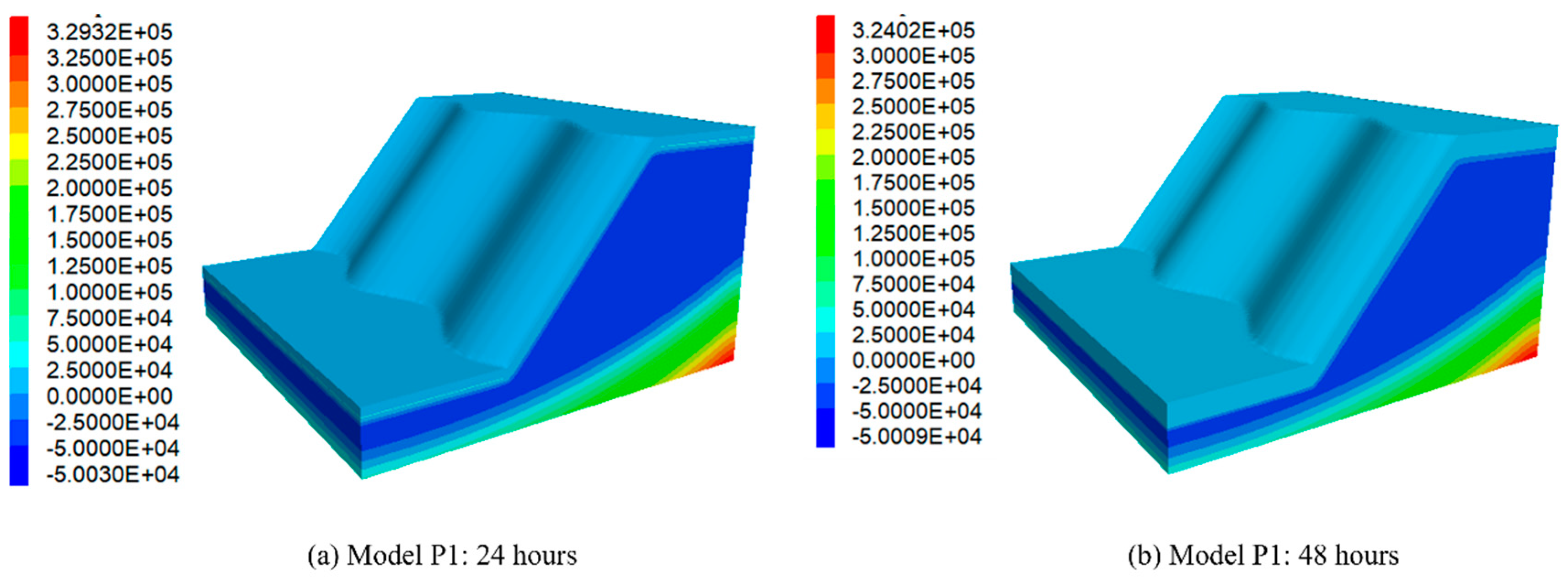
Figure 8. The pore pressure distribution in the slope after 24 h (a) and 48 h (b) of rainfall. The pore pressure on the slope surface was set to 0 when surface runoff formed.
Geohazards 05 00037 g008
Figure 9. (a) Top view of Model P2.1 (unit: m). (b) Side view of Model P2.1, and A, B is the groundwater level, and A, B, C, D is the unsaturated zone. (unit: m).
Geohazards 05 00037 g009
Figure 10. (a) Model P2.1 where the slope gradient increases from 40° to 64° in increments of 8° for each convex and concave section (unit: m). (b) Model P3.1 where the slope gradient increases from 40° to 58° in increments of 6° for each convex and concave section (unit: m).
Geohazards 05 00037 g010
Figure 11. (a) Side view of Model P3.1 with a slope gradient of 58° (unit: m). (b) Side view of Model P4.1 with a slope gradient of 49°, and A, B is the groundwater level, and A, B, C, D is the unsaturated zone. (unit: m).
Geohazards 05 00037 g011
Figure 12. (a) Top view of Model O3 (unit: m). (b) Side view of Model O3 with a gradient of 50°, and A, B is the groundwater level, and A, B, C, D is the unsaturated zone. (unit: m).
Geohazards 05 00037 g012
Figure 13. (a) Model O1 with an undulation frequency of 2; (b) Model O2 with an undulation frequency of 4; (c) Model O3 with an undulation frequency of 6; (d) Model O4 with an undulation amplitude of 5 m; and (e) Model O5 with an undulation amplitude of 15 m.
Geohazards 05 00037 g013
Figure 14. The maximum shear strain contours and factors of safety for Models P1 and P2 before rainfall and after 48 h of rainfall.
Geohazards 05 00037 g014
Figure 15. The maximum shear strain contours and factors of safety for Models P3 and P4 before rainfall and after 48 h of rainfall.
Geohazards 05 00037 g015
Figure 16. The maximum shear strain contours and factors of safety for Models P1.1 and P2.1 before rainfall and after 48 h of rainfall.
Geohazards 05 00037 g016
Figure 17. The maximum shear strain contours and factors of safety for Models P3.1 and P4.1 before rainfall and after 48 h of rainfall.
Geohazards 05 00037 g017
Figure 18. Difference in the factor of safety for different increments of undulation degrees.
Geohazards 05 00037 g018
Figure 19. Difference in the factor of safety for different increments of slope gradients.
Geohazards 05 00037 g019
Figure 20. The maximum shear strain contours and factors of safety for Models O1, O2 and O3 before rainfall and after 48 h of rainfall.
Geohazards 05 00037 g020
Figure 21. The maximum shear strain contours and factors of safety for Models O4 and O5 before rainfall and after 48 h of rainfall.
Geohazards 05 00037 g021
Figure 22. Difference in the factor of safety for different frequencies of undulation.
Geohazards 05 00037 g022
Figure 23. Difference in the factor of safety for different degrees of undulation (m).
Geohazards 05 00037 g023
Table 1. The geological data of the Sasebo landslide.
StratumDesignationClassificationDescription
Quaternary Colluvial soilDtSandy soilCoarse-grained soil with sub-angular gravel of sandstone.
NeogeneWeathered sandstoneWSsWeathered rockThe hardness of weathered rock allows it to be broken with light hammer strikes.
Weathered MudstoneMsSoft rockFragile mudstone interlayered with weathered sandstone. Some parts of the core are so weakened that they can be crumbled by hand.
SandstoneSsSoft rockFresh fine-grained sandstone. The hardness of rock allows it to be broken under medium hammer strikes.
Table 2. The material properties of the slope in the saturated state.
Friction Angle
°
Cohesion
kPa
Poisson’s RatioDensity
kg/m3
Young’s Modulus
MPa
Permeability
m/s
Strongly weathered sandstone38600.3618002006 × 10−6
Moderately weathered sandstone40800.3021003001 × 10−6
Bedrock421000.3022006005 × 10−7
Table 3. Stability of 3D slopes with different undulation degrees and slope gradients.
GroupModelUndulation Degrees (m)
Slope Gradient (50°)
FoS
Rainfall Duration (h)
DF (%)
0 h24 h48 h0 h24 h48 h
1P15, 5, 5, 52.1331.6291.3953.540.999.84
P25, 7, 9, 112.1481.6131.3674.270.007.64
P35, 8, 11, 142.061.501.3160.00−7.013.62
P45, 9, 13, 171.9491.421.27−5.39−11.970.00
2D analysis (slope gradient: 50°)2.061.6131.27
Variation of slope gradients (°)
2P1.140, 48, 56, 641.781.3401.19512.235.5116.02
P2.140, 48, 56, 641.771.331.1911.604.7215.53
P3.140, 46, 52, 581.9341.4611.2859.273.0313.42
P4.140, 43, 46, 492.091.5271.3322.50−5.165.55
2D analysis492.0391.611.262
581.771.4181.133
641.5861.2701.03
Table 4. Stability of 3D slopes with different undulation degrees and frequencies.
GroupModelFrequenciesDegrees (m)FoS
Rainfall Duration (h)
DF (%)
0 h24 h48 h0 h24 h48 h
4O12102.0081.5121.324−2.58−6.484.83
O24101.981.4101.242−4.04−14.18−1.45
O36102.0081.3671.180−2.58−17.78−6.78
2D analysis2.061.611.26
5O4452.1331.6291.3833.421.168.89
O54151.771.2461.10−16.4−29.21−14.54
Disclaimer/Publisher’s Note: The statements, opinions and data contained in all publications are solely those of the individual author(s) and contributor(s) and not of MDPI and/or the editor(s). MDPI and/or the editor(s) disclaim responsibility for any injury to people or property resulting from any ideas, methods, instructions or products referred to in the content.