Abstract
Offshore basalts, most commonly found as oceanic crust formed at mid-ocean ridges, are estimated to offer an almost unlimited reservoir for CO2 sequestration and are regarded as one of the most durable locations for carbon sequestration since injected CO2 will mineralize, forming carbonate rock. As part of the Solid Carbon project, the potential of the Cascadia Basin, about 200 km off the west coast of Vancouver Island, Canada, is investigated as a site for geological CO2 sequestration. In anticipation of a demonstration proposed to take place, it is essential to assess the tendency of geologic faults in the area to slip in the presence of CO2 injection, potentially causing seismic events. To understand the viability of the reservoir, a quantitative risk assessment of the proposed site area was conducted. This involved a detailed characterization of the proposed injection site to understand baseline stress and pressure conditions and identify individual faults or fault zones with the potential to slip and thereby generate seismicity. The results indicate that fault slip potential is minimal (less than 1%) for a constant injection of up to ~2.5 MT/yr. This is in part due to the thickness of the basalt aquifer and its permeability. The results provide a reference for assessing the potential earthquake risk from CO2 injection in similar ocean basalt basins.
1. Introduction
The Solid Carbon project plans to inject CO2 into sub-seafloor basalt, where it will mineralize, forming solid carbonate rock for durable carbon sequestration [1]. The proposed injection site is about 200 km off the west coast of Vancouver Island, British Columbia, Canada, in the Cascadia Basin (Figure 1). When coupled with CO2 capture or direct air carbon removal, geologic carbon sequestration is a valuable strategy to reduce CO2 emissions and lower concentrations in the atmosphere [1]. The Cascadia Basin was identified by [2] as an area that offers a large capacity of CO2 storage volumes. The criteria they used as a screening tool for site selections required that the oceanic crust around the proposed injection site must be young for optimal mineralization, sediment thickness must be greater than 200 m to form an effective caprock, water depths must be greater than 3000 m to prevent any leaked CO2 from reaching the atmosphere, and porosity and permeability must be ~10–20% and 0.1–1 D, respectively [1]. Additionally, simulations indicate that a 50 MMT CO2 plume injected over a 20-year period will remain within the reservoir area, both laterally and vertically, at least 50 years after injection stops. One of many modelling results showed that the CO2 is fully converted to solid rock within ~135 years or less after injection ceases [1,3].
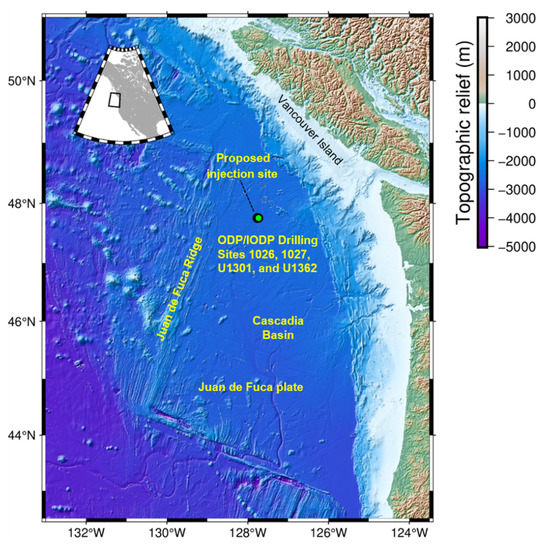
Figure 1.
Location of proposed injection site for the Solid Carbon project in the Cascadia basin.
As with other injection projects, a careful site characterization is required to assess the region to understand what controls the possible occurrence and behavior of induced seismicity. Hence, this study is aimed at understanding the effect of induced seismicity in and around the injection site. Induced seismicity is earthquakes resulting from human activities. These activities include mining, dam impoundment, carbon capture and sequestration (CCS), hydraulic fracturing, geothermal systems, and waste fluid disposal [4,5,6,7]. The main physical mechanism responsible for triggering injection-induced seismicity is an increase in pore pressure on fault surfaces, which decreases the effective normal stress, effectively unclamping the fault and allowing slip initiation [8]. Hence, to induce seismicity, there must be sufficient pore pressure buildup, faults that are susceptible to slip, and a pathway allowing the increased pressure to communicate with the fault.
Due to the paucity of induced seismicity data related to CCS projects worldwide, references to past studies involving water injection can be considered. There are many similarities between CCS and wastewater disposal [9,10]. Hence, we can examine past cases of wastewater disposal-induced seismicity to improve our understanding of the CCS project. However, differences with CCS need to be taken into account, such as the depth of injection, types of rock in which injection takes place, and injection pressure, volume, and duration. Since fluid injection induces seismicity by increasing pore pressure [8], an evaluation of pressure increases is vital in monitoring induced seismicity at CCS sites. According to [11], to assess whether CO2 injection can induce perceivable seismicity, the first step is to carry out a detailed initial site characterization. This study describes such a site characterization and the results for fault slip potential for the Cascadia Basin, where the injection is proposed as part of the Solid Carbon project. This evaluation involves considering the Gutenberg–Richter frequency–magnitude distribution [12] to understand the background seismicity at the site, as well as characteristics of geological formations and faults, including their location and orientation through available seismic data, with the goal of building a conceptual model to understand pressure levels that could be allowed during actual CO2 injection. Previous studies of similar modelling have focused on onshore cases of induced seismicity risk assessment. In this study, we incorporated calculations that will accommodate the effects of pore pressure increase in an offshore setting.
2. Geological Setting
The proposed injection site is within the ocean basalt of a relatively heavily sedimented region of the Cascadia Basin. In particular, the sediments on the eastern flank of the Juan de Fuca Ridge are young in age but thick due to the high rate at which sediments are supplied by the adjacent North American continent [13]. Topographic relief associated with the Juan de Fuca Ridge axis and abyssal hill bathymetry on the ridge flank has helped to trap turbidites flowing west from the continental margin [14]. Regional basement relief is dominated by linear ridges and troughs (Figure 2c) oriented subparallel to the spreading centre and produced mainly by faulting, variations in magmatic supply at the ridge, and off-axis volcanism [14,15]. The basalt in this region is potentially well suited to CO2 sequestration [1]. Permeability is on the order of 0.1 to 1 D within the uppermost 600 m of the basaltic crust. Porosity values of 10–20% were inferred from bulk density logs. Fine-grained sediments overlying the basalt are nearly continuous and provide a low-permeability barrier separating the storage reservoir from the overlying ocean.
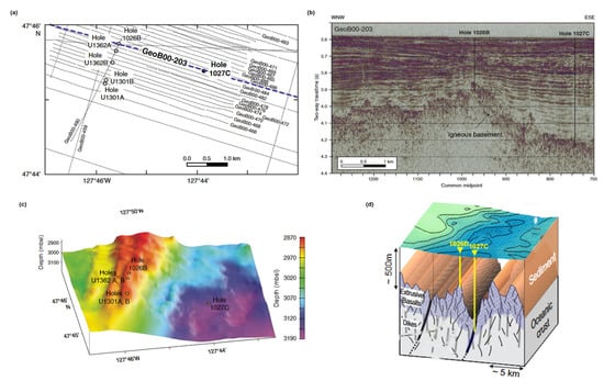
Figure 2.
(a) Seismic line map showing Line Geob00-203 across Holes 1026B and 1027C. (b) Seismic Line Geoboo-203 across Holes 1026B and 1027C showing sediment/basalt interface and steeply dipping normal faults to the west of Hole 1026B. Modified from [15]. (c) Basement relief map showing hole locations. Modified from [16]. (d) Schematic illustration of the injection site showing tectonic features. Modified from [17].
3. Data and Methods
In this section, we begin the site characterization by first looking at past seismicity data. The next step is to carry out a geomechanical characterization using the stress data. This is followed by pore pressure modelling. Finally, the fault slip potential is calculated by combining results from both the geomechanical and hydrologic models (Section 5).
3.1. Historical Seismicity Data
Historical data are needed to establish the background rate of naturally occurring seismic events in a particular area over a period of time [4]. This helps to establish the baseline of natural seismicity, which in turn can help to determine whether any increases in seismicity after injection are due to natural causes or human activities. For this purpose, earthquake data were compiled from the Incorporated Research Institutions for Seismology (IRIS) Data Management Centre through the FDSN web service in ZMAP. Historical earthquake data between 1 January 2012 and 1 July 2022 indicate that the proposed injection site is relatively quiescent, and the majority of earthquakes occur along the Juan de Fuca Ridge axis, Blanco Fracture Zone, and transform fault to the south, as well as on the Explorer Plate to the north (Figure 3). Most of the earthquakes in this area appear at depths of 10 km and greater, but depths are poorly constrained. The earthquake magnitude distributions around the proposed injection site are considered using the Gutenberg–Richter relationship, with results described in Section 4.
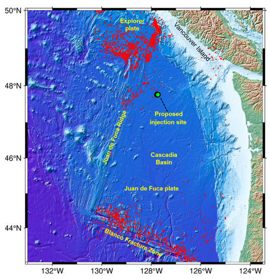
Figure 3.
Distribution of seismicity (red dots) around the Cascadia basin from 1 January 2012 to 1 July 2022.
3.2. Stress Data
To assess whether CCS operations could induce fault slip, we first determine the initial in situ stress field. No published stress data are presently available for the proposed injection site. We assessed formation micro scan (FMS) and formation micro imager (FMI) logs from the Integrated Ocean Drilling Program (IODP) Holes U1301B and U1362A (Figure 4). The stratigraphy indicated mainly pillow basalt, and no breakouts were observed. However, a horizontal compressive stress regime was inferred from breakout orientations from logging while drilling and wireline data at the northern Cascadia margin [18]. The maximum horizontal compressive stress SHmax is generally margin-normal, which is consistent with the direction of plate convergence. The researchers of [19] published similar results from analysis of earthquake focal mechanism data.
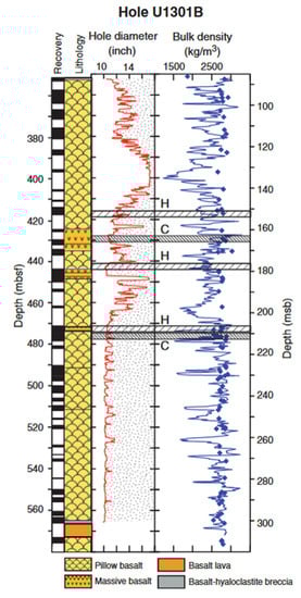
Figure 4.
Stratigraphy, hole diameter, and bulk density logs from Hole U1301B (See Figure 2 for location). The depth (mbsf) denotes metres below seafloor. Modified from [14].
The vertical stress gradient (Sv) was calculated based on well-log density data (Figure 4) from Hole U1301B, given as 2.65 g/cm3 for a depth of 400 m below seafloor (mbsf), the approximate depth of the injection zone within the basalt [14]. The pore pressure gradient was calculated by assuming that pressure is hydrostatic, and using a seawater density of 1.03 g/cm3.
3.3. Fault Data
To build the fault data set, we considered interpreted faults from 2D single-channel seismic reflection data (Figure 5) compiled from Ocean Drilling Program (ODP) Leg 168 [20,21] and from multichannel seismic data around Holes 1027 and 1026 from Cruise EW0207 [22] and Cruise MGL1211-02 [23], respectively, as well as from published, interpreted seismic sections [16,24,25].
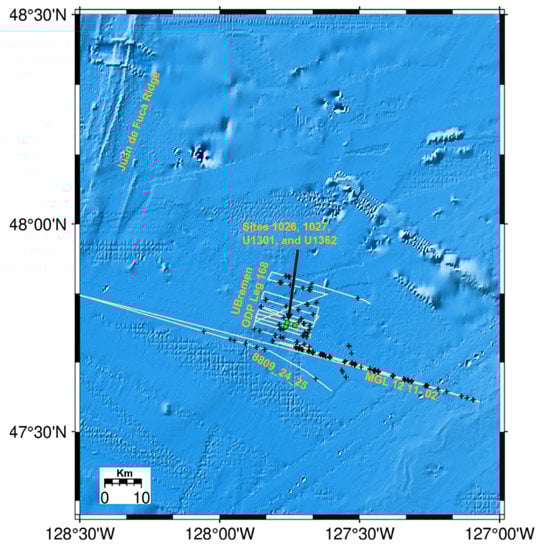
Figure 5.
Location map showing the fault picks (crosses) used for the FSP modelling and 2D single-channel seismic reflection lines across the proposed injection site. The fault picks had previously been extracted using the Kingdom Suite software. The fault picks had precise (latitude and longitude) location markers and were then imported into the FSP software for modelling.
We used a probabilistic distribution of strikes and dips considering that the interpreted faults are sub-parallel to the magnetic lineations; faults and fractures are aligned in the direction of the ridge at N80°E [17,24,25]; and the Juan de Fuca plate has extensional fault blocks [26]. A conservative assumption was made for the fault dips within the generally normal extensional faulting environment. The faults within the ridge are high-angle extensional faults; hence, the faults were given a dip range of 60° to 78° [16,24].
Our fault model includes 131 faults, each defined by two connected coordinate points and interpreted to root into the igneous basement (Figure 2b). The faults segments had previously been extracted using the Kingdom Suite software and represented the top and bottom of the fault pick times. The fault picks from the bottom segments are interpreted travel times within the basement. This suggests that the majority of the faults penetrate the basement fabric. Analysis of the fault slip potential requires knowledge of fault orientations and in situ stress orientations and magnitudes in addition to an assumption for the coefficient of friction µ. Previous research has shown that, for different rock types, µ ranges from 0.6 to 1.0 for effective normal stresses of <100 MPa [27]. When assessing the fault slip potential, a critical value for the friction coefficient is typically 0.6 [28,29,30]. Hence, the coefficient of friction was chosen here to be 0.6.
3.4. Mohr–Coulomb Failure Criteria
The Mohr–Coulomb failure criteria are used to determine how large stress perturbations must be to trigger induced seismicity. The stress conditions on the fault need to be known, and are usually also estimated using the Mohr–Coulomb criterion. If the shear stress, exceeds the Coulomb criterion given by
then the fault will be activated. In Equation (1), µ is the coefficient of static friction, σn is the normal (compressive) stress on the fault, and P is the total pore pressure, given as
where is the initial pore pressure (hydrostatic pressure), and ΔP is the excess pore pressure caused by fluid injection. Under normal conditions, the effective normal stress, which is oriented normal to the fault plane, reduces the likelihood of slip occurring on the fault by clamping the fault closed. During fluid injection, however, the pore fluid pressure increases, with the effective normal stress decreasing proportionally, thereby unclamping the fault, which may lead to slip. Thus, we can calculate in a deterministic manner the pore pressure needed to cause a stable fault to slip [31].
The minimum and maximum horizontal stresses are constrained here using an Aϕ parameter of 0.7 [32,33], which indicates a normal/strike–slip faulting regime. This parameter quantifies both the shape factor and the Andersonian faulting type [34]. The lower and upper bounds of the horizontal stresses can be determined based on Anderson’s faulting theory [35].
4. Frequency Magnitude Distributions
Earthquakes typically follow the Gutenberg–Richter relationship [12], which can be expressed as
where N(M) is the cumulative number of earthquakes of magnitude larger than a given magnitude M. The parameter b represents the absolute value of the negative slope of the magnitude relationship, and describes the distribution of small to large earthquakes in a particular sample [12]. Analyses from laboratory studies, mines, and numerical simulations show that the b value depends on stress conditions [36]. The parameter a is proportional to the seismic productivity. Here, b values are estimated using the maximum likelihood formulation of [37] and the magnitude of completeness (Mc), employing the maximum curvature method [38] with the aid of the ZMAP software package [39].
Mc represents the magnitude at which the lower end of the Gutenberg–Richter relationship departs from the frequency–magnitude data, indicating incomplete data for earthquakes at lower magnitudes. Events of magnitude M < Mc are discarded from further analysis [40]. Using the frequency–magnitude data and completeness magnitude shown in Figure 6, the b value was calculated using Equation (3) to be 0.85 ± 0.07, which is typical of the general tectonic environment of the Cascadia Basin [41,42,43].
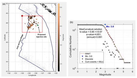
Figure 6.
Frequency–magnitude distribution of earthquakes in the Cascadia basin from 1 January 2012 to 1 July 2022. (a) Distribution of seismicity around the proposed injection site (red box inset). The colour scale represents the magnitude. (b) Gutenberg–Richter log for earthquakes in the red box region.
5. Fault Slip Potential Analysis
The FSP v. 2.0 software package, developed by the Stanford Center for Induced and Triggered Seismicity, is a freely available integrated reservoir geomechanics software modelling tool [44]. In this study, FSP was used to estimate the chance of a fault slipping under certain sets of conditions (scenarios). FSP is best suited for the study area with no known stress details by using an interpolated and smooth stress field, and probabilistically determines the fault slip potential. The model uses input parameters describing the stress, hydrology, fault, and injection well rates (Table 1). FSP is based on the Mohr circle failure criterion and allows either a deterministic or probabilistic geomechanical analysis of the fault slip potential. The probabilistic geomechanical analysis implements a Monte Carlo simulation, allowing uncertainties in input parameters to be propagated through the model.

Table 1.
Parameters and data needed to define the stress tensor, geomechanical model, and hydrologic model.
Our method is to probabilistically estimate fault slip potential using two scenarios: a hydrostatic (control) case representing the conditions prior to injection, and a case representing a plausible increase in pore fluid pressure that can be used to assess the general hazard of CO2 injection.
5.1. Deterministic Analysis of the Fault Slip Potential
The deterministic analysis of the slip potential for the faults in the absence of fluid injection was first calculated. All stress and pressure values are entered as gradients (in psi/ft) at a specified reference depth. The parameters used for the analysis are the vertical stress gradient given as 1.15 psi/ft (25.97 MPa/km). The initial hydrostatic pressure gradient is 0.45 psi/ft (10.1 MPa/km). An Aϕ parameter of 0.7 was used for a normal stress regime. The reference depth for these calculations is 9843 ft (3000 m), which is the depth of the uppermost part of the basalt rock. As explained above, we used a critical coefficient of friction of μ = 0.6 with the orientation of the maximum principal stress as N80°E. The Mohr–Coulomb failure criteria were applied to assess the initial stable state of the fault slip.
Figure 7 shows the results of the deterministic analysis of the pore pressure required to generate slip for each fault in the hydrostatic case, which varies with the different fault strikes and SHmax orientations. It is found that the majority of the faults are unlikely to slip in the hydrostatic stress field. For faults of concern (coloured red in Figure 7), a pore pressure increase of 200 to 1200 psi ( is needed to initiate slip. The faults coloured yellow are likely to slip in response to a pore pressure increase of 1300 to 2800 psi (
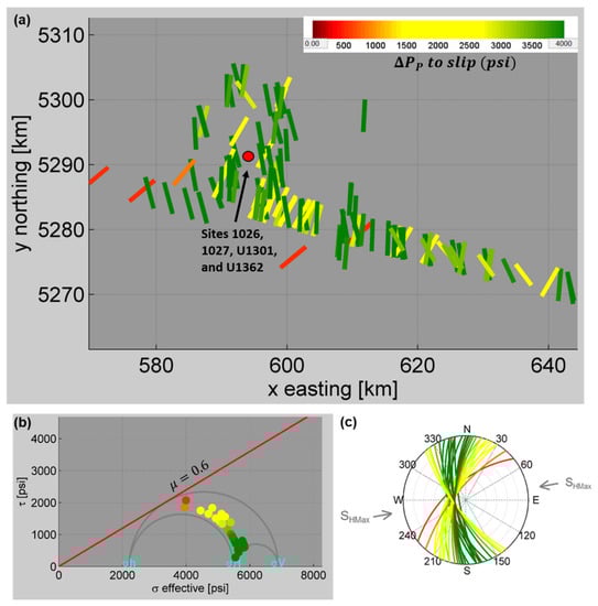
Figure 7.
Initial stability of the faults for the hydrostatic case at a reference state of stress at 3 km depth, assuming a normal stress regime with Aϕ = 0.7. (a) Map view of the faults with the horizontal distance to slip in psi represented using the colour scale. (b) Mohr diagram of the conceptual fault model, where the horizontal axis is the effective compressive stress and the vertical axis is the shear stress. The dots show reference stress conditions for the fault orientations with colours as in (a). The pore pressure to slip for each fault is the horizontal distance from the fault stress state point to the red frictional line. The principal stresses are labelled in cyan. (c) Stereonet representation of the faults with grey arrows denoting the direction of the maximum horizontal stress direction.
As shown in Figure 7, in both the Mohr circle and stereonet representations, the red fractures are optimally oriented for failure, while the green fractures are far from failure. If we group the faults based on the colours, the slip tendency, as well as the proximity of the resolved stresses to the Mohr–Coulomb failure criterion, failure depends on the orientation of the fault with respect to the stress field. The majority of the faults (green) are oriented almost 87° from SHmax. The red fractures are oriented at about 34°, while the yellow fractures are oriented at ~65° from SHmax.
5.2. Probabilistic Analysis of Fault Slip Potential
The conditional probability of failure given the in situ stress field can be determined through a quantitative risk assessment (QRA) methodology [31,47]. Following the approach of [31], we also carried out a probabilistic analysis of the fault slip potential, based on 1000 Monte Carlo realizations, to address uncertainties that are present in the data (Figure 8). A probabilistic analysis is performed to take into account the uncertainties in the input parameters. In the common case of onshore calculations, the stress gradients are multiplied by the reference depth. For the offshore case, we take into account the presence of the overlying water weight. Hence, we applied an error of ±0.17 psi/ft to the vertical and hydrostatic pore pressure gradients, which is the error that results from including the overlying water weight. The fault strike and dip angles have uncertainties of ±10°. The coefficient of friction, which is the same for all the faults, was given an uncertainty of ±0.01, and the direction of the maximum horizontal stress had an uncertainty of ±10°. These values represent reasonable assumptions since no stress data were available.
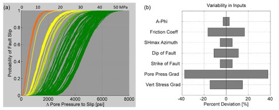
Figure 8.
Example of the probabilistic analysis of fault slip potential. (a) Probability of fault slip as a function of pore pressure increase on each fault (coloured as in Figure 7). (b) Uncertainties in the fault slip potential analysis variables are shown as percentages.
Figure 8 shows the result of the probabilistic analysis, indicating that the probability of failure does not exceed 80% until the pore-pressure change is in excess of 3000 psi (~21 MPa) for fractures not critically stressed (in green). However, fractures closer to failure (in red) require a pore pressure of ~1000 psi (7 MPa) to give the same probability of failure.
5.3. Fault Slip Potential Due to Fluid Injection
In this section, we calculate the probability of the fault slipping in response to a CO2 injection rate of 2.5 Mt/year for 10 years. The hydrological parameters used for modelling are the aquifer thickness, porosity, and permeability of the injection layer. In Figure 9, two aquifer thicknesses are modelled: 100 m and 300 m, with an average porosity of 10% and a permeability of 0.322D [45,46]. One injection well with a rate of ~6814 metric tons a day was used in this study over 10 years. We assume in the model that the pressure in the aquifer is initially uniform. The permeability, fluid and rock compressibility, and viscosity are constant.
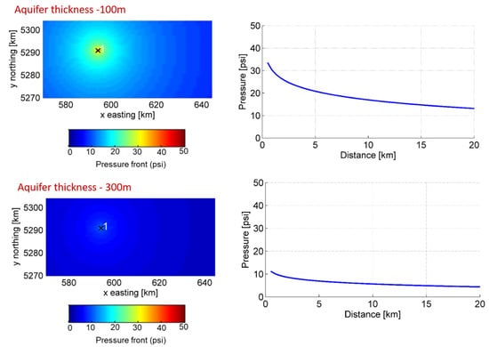
Figure 9.
Fluid pressure perturbation from the injection well and pressure increase (blue curves) plotted as a function of distance from the well after 10 years of injection of CO2 using a volumetric rate of 6814 m3/day at reservoir conditions into the basalt formation 3000 m below the sea surface. The formation permeability is 0.322 D, and thickness shown is for 100 m (upper panel) and 300 m (lower panel).
5.4. Assessment of the Fault Slip Potential
The geomechanics and hydrology models are combined to give the fault slip potential for all the faults in Figure 10.
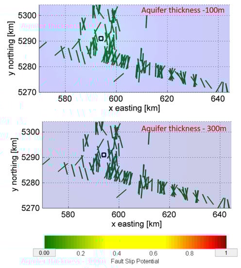
Figure 10.
Fault slip potential due to a constant injection in a basalt aquifer 100 m (upper panel) and 300 m (lower panel) thick with an injection rate of 2.5 MT of CO2 over 10 years. The fault traces are coloured by their slip potential. In this case, all the faults are green, indicating a minimal slip potential of ~0.01.
6. Discussion
6.1. Effect of the Stress Field and Fault Orientation on the Fault Slip Potential
Sufficient pore pressure increases are required during fluid injection to cause fault slip. In addition, fault slip in response to injection usually depends on factors such as the orientation and magnitude of the stress field, the fault orientation, and the coefficient of friction. Quantitative risk assessment (QRA) is used to evaluate these parameters based on their uncertainties [31]. For the stress field analysis, FMS well logs around the proposed injection site were examined for breakout patterns. No breakout patterns were observed; the few dark patches in the logs were interpreted to be reflections at the boundaries of the pillow basalt stratigraphy. Best estimates for SHmax orientation were interpreted based on analogs from the Nankai trough and Chile triple junction convergent margins, and taking into account regional trends within the Cascadia Basin. The tectonics of the surrounding region in southwest British Columbia are complex due to the locked Cascadia subduction zone, the change in the strike of the margin, and the bend in the subducting plate [19].
The orientation of a fault with respect to the local stress fields can have a significant influence on the likelihood of slip occurrence. Faults that are nearly perpendicular to SHmax are unlikely to slip in the normal/strike–slip faulting stress regime [47]. Tectonic plate movements are the main contributors to the direction of maximum horizontal stress. Considering that the proposed injection site is located between the mid-ocean ridge spreading centre and far from the subduction fault, we propose SHmax to be in the WSW-ENE orientation. The SHmax orientations typically do not change significantly with depth [31,48]. Hence, this SHmax orientation was assumed for both the sediment and oceanic basalt.
The ridge has many extensional faults, which were compiled from seismic data; hence, we assume a value of Aϕ of 0.7 for a normal to strike–slip stress regime [32,33]. Anderson’s fault type characterized the three types of faulting as normal, strike–slip, and reverse, which depends on the stress tensor and its orientation relative to the earth’s surface. Knowledge of the Aϕ parameter can be used to infer the stress regime in the absence of complete information on the actual values of the stresses [34].
In Figure 7c, faults that are oriented almost parallel to SHmax are more oriented for failure when compared with faults almost perpendicular to SHmax. In our study area, the majority of the faults are parallel to the ridge axis [17], with SHmax almost in the E-W direction. Taken together, these results indicate that the faults at our study site are less likely to slip.
6.2. Effect of Aquifer Thickness and Injection Rate on the Fault Slip Potential
Fault instability, in general, increases as the distance decreases between the injection well and a fault [49]. In Figure 9, the excess pore pressure that occurs over a 10-year time period is modelled. The results show that the reservoir thicknesses directly affect the distribution of excess pore pressure caused by fluid injection. The inferred increased bottom hole pressure for this study is about 30 psi (0.21 MPa) for an aquifer thickness of 100 m and approximately 10 psi (0.1 MPa) for a thickness of 300 m. The basalt aquifer for our study is permeable and about 300 m thick [45,46]. A similar low bottom hole pressure of ~15 psi (0.1 MPa) was found in the case of CO2 injection in Sleipner, Norway [4]. The reservoir has a thickness of about 300 m around the injection site [50] with an average injection rate of 0.85 MT/yr. In our study, the excess pore pressure is also minimal due to the thickness of the basalt aquifer.
6.3. Effect of Pore Pressure Perturbations on the Fault Slip Potential
FSP was used in this study to investigate whether increases in pore pressure from the CO2 injection could induce fault slip. The combined fault slip potential for both the geomechanical and hydrological modelling is shown in Figure 10. The result shows that the effect on the FSP is very low (0.01). This is partly due to the low pressure change in the midpoint of the fault.
7. Conclusions
One of the key considerations for safe and secure geologic storage of CO2 is the detailed characterization of the injection site to understand baseline stress and pressure conditions and to identify individual faults or fault zones of concern that are likely to slip and thereby generate seismicity. The FSP tool is used to investigate whether increases in pore pressure from a CO2 injection into the basalt aquifer could induce fault slip. This research is novel in the sense that this would be the first application of the FSP tool to an offshore marine case. Previous studies were limited to land. The evaluation methods took into account calculations from an oceanic setting. The conditional probability of failure, given the in situ stress field, was determined through a quantitative risk assessment methodology using the FSP software [31]. The fault slip modelling shows that variations in the orientation of the maximum horizontal compressive stress SHmax can significantly change the fault slip potential. However, the FSP software accommodates variations in stress orientation.
Our modelling shows that the effect of injecting 2.5 MMT of CO2 for 10 years on the fault slip potential is minimal (less than 0.01. The fault slip potential modelling can be used as a proxy for the likelihood of failure for a given fluid pressure increase. One recommendation is to continuously measure pore pressure changes during injection to remain well below threshold limits.
Author Contributions
Formal analysis, E.E.J.; methodology, E.E.J.; fault interpretation, K.M.R.; writing—original draft preparation, E.E.J.; writing—review and editing, E.E.J., M.S., K.M., S.E.D. and K.M.R.; visualization, E.E.J.; Supervision, M.S., K.M. and S.E.D. All authors have read and agreed to the published version of the manuscript.
Funding
We acknowledge the support of the Pacific Institute for Climate Solutions to the Solid Carbon initiative through its Theme Partnership Program.
Acknowledgments
We are grateful for support from the Pacific Institute for Climate Solutions. We thank Michael Riedel and Angela Slagle for their help in evaluating the borehole data.
Conflicts of Interest
The authors declare no conflict of interest.
References
- Goldberg, D.; Aston, L.; Bonneville, A.; Demirkanli, I.; Evans, C.; Fisher, A.; Garcia, H.; Gerrard, M.; Heesemann, M.; Hnottavange-Telleen, K.; et al. Geological Storage of CO2 in Sub-Seafloor Basalt: The CarbonSAFE Pre-Feasibility Study Offshore Washington State and British Columbia. Energy Procedia 2018, 146, 158–165. [Google Scholar] [CrossRef]
- Goldberg, D.; Slagle, A.L. A Global Assessment of Deep-Sea Basalt Sites for Carbon Sequestration. Energy Procedia 2009, 1, 3675–3682. [Google Scholar] [CrossRef]
- Awolayo, A.N.; Laureijs, C.T.; Byng, J.; Luhmann, A.J.; Lauer, R.; Tutolo, B.M. Mineral Surface Area Accessibility and Sensitivity Constraints on Carbon Mineralization in Basaltic Aquifers. Geochim. Cosmochim. Acta 2022, 334, 293–315. [Google Scholar] [CrossRef]
- Ground Water Protection Council and Interstate Oil and Gas Compact Commission. Potential Induced Seismicity Guide: A Resource of Technical & Regulatory Considerations Associated with Fluid Injection, 2nd ed.; Ground Water Protection Council: Oklahoma City, OK, USA, 2021; p. 250. [Google Scholar]
- Grigoli, F.; Cesca, S.; Priolo, E.; Rinaldi, A.P.; Clinton, J.F.; Stabile, T.A.; Dost, B.; Fernandez, M.G.; Wiemer, S.; Dahm, T. Current Challenges in Monitoring, Discrimination, and Management of Induced Seismicity Related to Underground Industrial Activities: A European Perspective. Rev. Geophys. 2017, 55, 310–340. [Google Scholar] [CrossRef]
- National Research Council. Energy. In Induced Seismicity Potential in Energy Technologies; National Academies Press: Washington, DC, USA, 2013; ISBN 9780309253703. [Google Scholar]
- Ellsworth, W.L. Injection-Induced Earthquakes. Science 2013, 341, 1225942. [Google Scholar] [CrossRef]
- Eaton, D.W. Passive Seismic Monitoring of Induced Seismicity; Cambridge University Press: Cambridge, UK, 2018; ISBN 9781107145252. [Google Scholar]
- Verdon, J.P. Significance for Secure CO2 Storage of Earthquakes Induced by Fluid Injection. Environ. Res. Lett. 2014, 9, 064022. [Google Scholar] [CrossRef]
- Verdon, J.P.; Stork, A.L. Carbon Capture and Storage, Geomechanics and Induced Seismic Activity. J. Rock Mech. Geotech. Eng. 2016, 8, 928–935. [Google Scholar] [CrossRef]
- Vilarrasa, V.; Carrera, J.; Olivella, S.; Rutqvist, J.; Laloui, L. Induced Seismicity in Geologic Carbon Storage. Solid Earth 2019, 10, 871–892. [Google Scholar] [CrossRef]
- Gutenberg, B.; Richter, C.F. Frequency of Earthquakes in California. Bull. Seismol. Soc. Am. 1944, 34, 185–188. [Google Scholar] [CrossRef]
- Bonifacie, M.; Monnin, C.; Jendrzejewski, N.; Agrinier, P.; Javoy, M. Chlorine Stable Isotopic Composition of Basement Fluids of the Eastern Flank of the Juan de Fuca Ridge (ODP Leg 168). Earth Planet. Sci. Lett. 2007, 260, 10–22. [Google Scholar] [CrossRef]
- Fisher, A.T.; Harris, M. Integrated Ocean Drilling Program Expedition 327 Preliminary Report: Juan de Fuca Ridge-Flank Hydrogeology the Hydrogeologic Architecture of Basaltic Oceanic Crust: Compartmentalization, Anisotropy, Microbiology, and Crustal-Scale Properties on the Eastern Flank of Juan de Fuca Ridge, Eastern Pacific Ocean, 5 July–5 September 2010. Available online: http://publications.iodp.org/preliminary_report/327/index.html (accessed on 30 April 2021).
- Fisher, A.T.; Urabe, T.; Klaus, A. IODP Expedition 301 Installs Three Borehole Crustal Observatories, Prepares for Three-Dimensional, Cross-Hole Experiments in the Northeastern Pacific Ocean. Sci. Drill. 2005, 1, 6–11. [Google Scholar] [CrossRef]
- Zühlsdorff, L.; Hutnak, M.; Fisher, A.T.; Spiess, V.; Davis, E.E.; Nedimovic, M.; Carbotte, S.; Villinger, H.; Becker, K. Site surveys related to IODP Expedition 301: ImageFlux (SO149) and RetroFlux (TN116) expeditions and earlier studies. InProc. IODP 2005, 301, 2. [Google Scholar]
- Sun, T.; Davis, E.; Heesemann, M. Seismic Formation Fluid Pressure Observations Reveal High Anisotropy of Oceanic Crust. Geophys. Res. Lett. 2021, 48, e2021GL095347. [Google Scholar] [CrossRef]
- Riedel, M.; Malinverno, A.; Wang, K.; Goldberg, D.; Guerin, G. Horizontal Compressive Stress Regime on the Northern Cascadia Margin Inferred from Borehole Breakouts. Geochem. Geophys. Geosyst. 2016, 17, 3529–3545. [Google Scholar] [CrossRef]
- Balfour, N.J.; Cassidy, J.F.; Dosso, S.E.; Mazzotti, S. Mapping Crustal Stress and Strain in Southwest British Columbia. J. Geophys. Res. 2011, 116, B03314. [Google Scholar] [CrossRef]
- Rosenberger, A.; Davis, E.E.; Villinger, H. Data report: Hydrocell-95 and-96 single-channel seismic data on the eastern Juan de Fuca Ridge flank. InProc. ODP Sci. Results 2000, 168, 9–19. [Google Scholar]
- Davis, E.E.; Fischer, A.T.; Firth, J.V. Hydrothermal Circulation in the Oceanic Crust: Eastern Flank of the Juan de Fuca Ridge: Covering Leg 168 of the Cruises of the Drilling Vessel JOIDES Resolution, San Francisco, California, to Victoria, British Columbia, Sites 1023–1032, 20 June–15 August 1996. In Proceedings of the Ocean Drilling Program. Part A, Initial report; Ocean Drilling Program: College Station, TX, USA; pp. 3235–3240. 1997; Volume 168, Available online: https://pascal-francis.inist.fr/vibad/index.php?action=getRecordDetail&idt=397608 (accessed on 30 April 2021).
- Carbotte, S.M.; Nedimović, M.R.; Canales, J.P.; Kent, G.M.; Harding, A.J.; Marjanović, M. Variable Crustal Structure along the Juan de Fuca Ridge: Influence of On-Axis Hot Spots and Absolute Plate Motions. Geochem. Geophys. Geosyst. 2008, 9, 8. [Google Scholar] [CrossRef]
- Carbotte, S.M.; Canales, J.P.; Carton, H.; Nedimović, M.R. Multi-Channel Seismic Shot Data from the Cascadia Subduction Zone Acquired during the R/V Marcus Langseth Expedition MGL1211(2012). In Integrated Earth Data Applications; IEDA: Des Moines, IA, USA, 2014; Available online: https://www.marine-geo.org/tools/search/Files.php?data_set_uid=19000 (accessed on 30 April 2021).
- Han, S.; Carbotte, S.M.; Canales, J.P.; Nedimović, M.R.; Carton, H.; Gibson, J.C.; Horning, G.W. Seismic Reflection Imaging of the Juan de Fuca Plate from Ridge to Trench: New Constraints on the Distribution of Faulting and Evolution of the Crust prior to Subduction. J. Geophys. Res. Solid Earth 2016, 121, 1849–1872. [Google Scholar] [CrossRef]
- Rohr, K.M.M.; King, H.; Riedel, M.; Schmidt, U. From mid-plate to subduction zone: Stratigraphy of the northeast Juan de Fuca plate, offshore British Columbia. Geol. Surv. Can. Curr. Res. 2019, 4. [Google Scholar]
- Ferguson, R.; King, H.M.; Kubik, K.; Rohr, K.M.; King, L.; Lister, C.J.; Fustic, M.; Hayward, N.; Brent, T.A.; Jassim, Y. Petroleum, mineral, and other resource potential in the offshore Pacific, British Columbia, Canada. Geol. Surv. Can. 2018, 1, 1. [Google Scholar]
- Byerlee, J. Friction of Rocks. Pure Appl. Geophys. PAGEOPH 1978, 116, 615–626. [Google Scholar] [CrossRef]
- Lund Snee, J.E.; Zoback, M.D. State of stress in Texas: Implications for induced seismicity. Geophys. Res. Lett. 2016, 43, 10–208. [Google Scholar]
- Lee, H.; Ong, S.H. Estimation of in situ stresses with hydro-fracturing tests and a statistical method. Rock Mech. Rock Eng. 2018, 51, 779–799. [Google Scholar] [CrossRef]
- Zhang, S.; Ma, X. Global frictional equilibrium via stochastic, local Coulomb frictional slips. J. Geophys. Res. Solid Earth 2021, 126, e2020JB021404. [Google Scholar] [CrossRef]
- Walsh, F.R.; Zoback, M.D. Probabilistic Assessment of Potential Fault Slip Related to Injection-Induced Earthquakes: Application to North-Central Oklahoma, USA. Geology 2016, 44, 991–994. [Google Scholar] [CrossRef]
- Lund Snee, J.-E.; Zoback, M.D. Multiscale Variations of the Crustal Stress Field throughout North America. Nat. Commun. 2020, 11, 1951. [Google Scholar] [CrossRef]
- Snee, J.-E.L.; Zoback, M.D. State of Stress in the Permian Basin, Texas and New Mexico: Implications for Induced Seismicity. Lead. Edge 2018, 37, 127–134. [Google Scholar] [CrossRef]
- Simpson, R.W. Quantifying Anderson’s Fault Types. J. Geophys. Res. Solid Earth 1997, 102, 17909–17919. [Google Scholar] [CrossRef]
- Zhang, Y.; Yin, S.; Zhang, J. In Situ Stress Prediction in Subsurface Rocks: An Overview and a New Method. Geofluids 2021, 2021, 6639793. [Google Scholar] [CrossRef]
- Farrell, J.; Husen, S.; Smith, R.B. Earthquake swarm and b-value characterization of the Yellowstone volcano-tectonic system. J. Volcanol. Geotherm. Res. 2009, 188, 260–276. [Google Scholar] [CrossRef]
- Aki, K. Maximum likelihood estimate of b in the formula log N= a-bM and its confidence limits. Bull. Earthq. Res. Inst. Tokyo Univ. 1965, 43, 237–239. [Google Scholar]
- Wiemer, S.; Wyss, M. Minimum Magnitude of Completeness in Earthquake Catalogs: Examples from Alaska, the Western United States, and Japan. Bull. Seismol. Soc. Am. 2000, 90, 859–869. [Google Scholar] [CrossRef]
- Wiemer, S. A Software Package to Analyze Seismicity: ZMAP. Seismol. Res. Lett. 2001, 72, 373–382. [Google Scholar] [CrossRef]
- Mignan, A.; Woessner, J. Estimating the magnitude of completeness for earthquake catalogs. Community Online Resour. Stat. Seism. Anal. 2012, 1–45. [Google Scholar]
- Wyss, M. Towards a Physical Understanding of the Earthquake Frequency Distribution. Geophys. J. Int. 1973, 31, 341–359. [Google Scholar] [CrossRef]
- Wiemer, S.; Benoit, J.P. Mapping the B-Value Anomaly at 100 Km Depth in the Alaska and New Zealand Subduction Zones. Geophys. Res. Lett. 1996, 23, 1557–1560. [Google Scholar] [CrossRef]
- Wiemer, S.; Wyss, M. Mapping spatial variability of the frequency-magnitude distribution of earthquakes. In Advances in Geophysics; Elsevier: Amsterdam, The Netherlands, 2002; Volume 45, p. 259. [Google Scholar]
- Walsh, R.; Zoback, M.D.; Lele, S.P.; Pais, D.; Weingarten, M.; Tyrrell, T. FSP 2.0: A Program for Probabilistic Estimation of Fault Slip Potential Resulting from Fluid Injection. 2018. Available online: https://scits.stanford.edu/fault-slip-potential-fsp (accessed on 30 April 2021).
- Winslow, D.M.; Fisher, A.T. Sustainability and Dynamics of Outcrop-to-Outcrop Hydrothermal Circulation. Nat. Commun. 2015, 6, 7567. [Google Scholar] [CrossRef] [PubMed]
- Winslow, D.M.; Fisher, A.T.; Stauffer, P.H.; Gable, C.W.; Zyvoloski, G.A. Three-Dimensional Modeling of Outcrop-to-Outcrop Hydrothermal Circulation on the Eastern Flank of the Juan de Fuca Ridge. J. Geophys. Res. Solid Earth 2016, 121, 1365–1382. [Google Scholar] [CrossRef]
- Chiaramonte, L.; Zoback, M.D.; Friedmann, J.; Stamp, V. Seal Integrity and Feasibility of CO2 Sequestration in the Teapot Dome EOR Pilot: Geomechanical Site Characterization. Environ. Geol. 2007, 54, 1667–1675. [Google Scholar] [CrossRef]
- Hennings, P.H.; Lund Snee, J.; Osmond, J.L.; DeShon, H.R.; Dommisse, R.; Horne, E.; Lemons, C.; Zoback, M.D. Injection-Induced Seismicity and Fault-Slip Potential in the Fort Worth Basin, Texas. Bull. Seismol. Soc. Am. 2019, 109, 1615–1634. [Google Scholar] [CrossRef]
- Goebel, T.H.W.; Brodsky, E.E. The Spatial Footprint of Injection Wells in a Global Compilation of Induced Earthquake Sequences. Science 2018, 361, 899–904. [Google Scholar] [CrossRef] [PubMed]
- Eiken, O. Twenty Years of Monitoring CO2 Injection at Sleipner. Geophysics and Geosequestration 2019, 209–234. [Google Scholar] [CrossRef]


Disclaimer/Publisher’s Note: The statements, opinions and data contained in all publications are solely those of the individual author(s) and contributor(s) and not of MDPI and/or the editor(s). MDPI and/or the editor(s) disclaim responsibility for any injury to people or property resulting from any ideas, methods, instructions or products referred to in the content. |
© 2023 by the authors. Licensee MDPI, Basel, Switzerland. This article is an open access article distributed under the terms and conditions of the Creative Commons Attribution (CC BY) license (https://creativecommons.org/licenses/by/4.0/).