2D Numerical Simulation of Floods in Ebro River and Analysis of Boundary Conditions to Model the Mequinenza Reservoir Dam

Abstract

The computational simulation of rivers is a useful tool that can be applied in a wide range of situations from providing real time alerts to the design of future mitigation plans. However, for all the applications, there are two important requirements when modeling river behavior: accuracy and reasonable computational times. This target has led to recent developments in numerical models based on the full two-dimensional (2D) shallow water equations (SWE). This work presents a GPU accelerated 2D SW model for the simulation of flood events in real time. It is based on a well-balanced explicit first-order finite volume scheme able to run over dry beds without the numerical instabilities that are likely to occur when used in complex topography. The model is applied to reproduce a real event in the reach of the Ebro River (Spain) with a downstream reservoir, in which a study of the most appropriate boundary condition (BC) for modeling of the dam is assessed (time-dependent level condition and weir condition). The whole creation of the model is detailed in terms of mesh optimization and validation. The simulation results are compared with field data over the flood duration (up to 20 days), allowing an analysis of the performance and time saved by different GPU devices and with the different BCs. The high values of fit between observed and simulated results, as well as the computational times achieved, are encouraging to propose the use of the model as a forecasting system.

1. Introduction

For centuries, natural disasters have been a source of concern for human beings due to the damage and losses they cause. In addition, in recent years, these losses and their frequency have been on the rise [1], leading to increased concern from governments, institutions and society in general. Within natural disasters, floods are one of the most destructive extreme events [2] and are the second leading cause of natural-disaster-related deaths in Spain, with 209 deaths between 2000 and 2019 [3]. They also entail a high expense due to damage repair, with losses in Spain amounting to EUR 12,000 million in the period between 2016 and 2020, with Zaragoza—located at NE of Spain—being the province with the third highest economic damage in the agricultural sector in this period. Figure 1 shows examples of such losses, demonstrating images of the surroundings of Zaragoza during flooding of the Ebro River, which is the largest river in terms of discharge in Spain. In view of these numbers, governments and public institutions require tools [4,5,6,7,8,9] and plans [10,11,12] to foresee and mitigate the damage caused by these events. One of these tools is the use of predictive models based on numerical simulations which are able to provide an accurate description of the spatial and temporal evolution of flow [13,14,15,16,17,18,19].

Due to the physical complexity of these phenomena, it is common to consider approximations to simplify the equations describing the flow. Although a river flood event is naturally a 3D problem, it is common to study it by averaging the equations in the vertical coordinate to reduce the problem to two horizontal dimensions [13,20]. Practical applications require a trade-off between spatial accuracy and computational efficiency [21], so approximations that reduce the dimensions of the problem are frequently used. The shallow water model (SWE) is a widely used approach to simulate surface geophysical flows in situations that involve large domains and long time scales [22,23,24]. This approach is based on the assumption that horizontal scales are larger than vertical scales, which leads to the possibility of neglecting vertical accelerations and assumes a hydrostatic pressure distribution in the vertical direction. This is the basis of the dynamic non-linear 2D SWE formulation. In some cases, the full dynamic equations are reduced in complexity by neglecting inertial terms. Reductions of the SWE system can be used to model floods with zero inertia models, which maintain the 2D framework and neglect terms that do not govern the phenomena, although special attention must be paid to their limits [25]. Further dimensional simplifications consider the average of the equations in the cross-section to reduce the formulation to a 1D approximation [14,26,27]. In large and complex flow domains, as is the case of a river in a flood event, two-dimensional models are the most frequently used to obtain the temporal and spatial description of the flow [13,20,21,25,28,29,30,31,32,33].

When modeling hydraulic structures present in the domain, the adopted different numerical strategies are of wide variety not only when these structures govern all the flow [34], but also if they only affect a part of the flow. For instance, when modeling complete reservoirs affecting a part of river, several strategies can be considered. On one hand, as the reservoir dynamics are close to quiescent equilibrium, some aggregated dimensionless models can be used to model their presence [35,36,37,38,39]. When more detail is required, the reservoir can be discretized [40] as a river extension by incorporating it to the computational domain and the dam presence is introduced via boundary conditions with a different hypothesis, as applied in this study.

To represent the behavior of a dam spillways, several boundary conditions can be used. If the main objective is to model the backwater generated by the dam, a constant water level with the main surface elevation of the reservoir can provide good results in terms of discharge and modeling the river. However, if the level of the reservoir is a variable to compute, which is a requirement of many applications focused on dam regulation, other, more sophisticated BCs must be applied. In particular, when the physical characteristics of the dam spillway are known, the outflow provided by the general discharge law of a dam spillway can be imposed as a boundary condition, so the backwater is still generated but the level is allowed to vary. Both strategies are analyzed in the this study.

Therefore, the main aim of this work is to study the region of the middle reach of the Ebro river between Zaragoza and Mequinenza, both located in Aragón (Spain), as seen in Figure 2. This region is not only of special interest due to the significant damage caused by large floods that occur in the meandering flood prone areas in the first half of the river in flood events, as seen in Figure 1a, but also because it contains a long reservoir, the Mequinenza reservoir, limited by the Mequinenza dam downstream. In this work, a 2D model is used for the discretization of both the river and the reservoir in order to compromise between computational efficiency and accuracy of the results. Therefore, the main objectives are to obtain an accurate computational model setup to study the Ebro River region and to optimize it, obtaining a predictive tool to foresee and mitigate potential damage caused by flooding events. Moreover, the presence of a reservoir allows the study of different boundary conditions that model dam spillways in order to obtain a realistic temporal evolution of the surface water level in the reservoir.

For the simulation, the PEKA2D program [16], developed at the University of Zaragoza, is applied to the mentioned river reach. A version of this program is included as computational core of the brand name RiverFlow2D^® (Hydronia LLC, https://www.hydronia.com/, accessed on 1 March 2023).

2. Governing Equations and Numerical Model

The governing equations and the numerical aspects of the scheme used can be found in full detail in [41,42] and it has been extended to 2D unstructured meshes in [20]. Their most important details are outlined in the following subsections.

2.1. 2D Shallow Water Equations

The mathematical model that describes the surface flow is given by the hyperbolic 2D shallow water system of equations based on mass and momentum conservation [43]:

$$\frac{\partial \mathbf{U}}{\partial t}+\frac{\partial \mathbf{F}\left(\mathbf{U}\right)}{\partial x}+\frac{\partial \mathbf{G}\left(\mathbf{U}\right)}{\partial y}=\mathbf{S}\left(\mathbf{U}\right)$$

(1)

where the conserved variables:

$$\mathbf{U}={\left(\begin{array}{ccc}h,& q_x,& q_y\end{array}\right)}^{\mathrm{T}}$$

(2)

are the water depth, h, and the unit discharge in x and y direction, $q_x=hu$ and $q_y=hv$, respectively, with $(u,v)$ being the depth averaged components of the velocity. The fluxes of these conserved variables are

$$\mathbf{F}\left(\mathbf{U}\right)={(hu, h{u}^2+\frac{1}{2}g{h}^2, huv)}^{\mathrm{T}}, \mathbf{G}\left(\mathbf{U}\right)={\left(\begin{array}{ccc}hv,& huv,& h{v}^2+\frac{1}{2}g{h}^2\end{array}\right)}^{\mathrm{T}}$$

(3)

The source term for the mass conservation equation is zero because neither precipitation, infiltration nor evaporation are included, assuming their contribution is practically negligible during a flooding event. Finally, the momentum source terms are related to the bed slopes and friction stresses:

$$\mathbf{S}\left(\mathbf{U}\right)={\left(\begin{array}{ccc}0,& gh(S_{ox}-S_{fx}),& gh(S_{oy}-S_{fy})\end{array}\right)}^{\mathrm{T}}$$

(4)

The bed slopes represent the variation in the x and y directions of the bottom level, $z_b$:

$$S_{ox}=-\frac{\partial z_b}{\partial x},S_{oy}=-\frac{\partial z_b}{\partial y}$$

(5)

and the friction stress components are given by:

$$S_{fx}=\frac{n^{2}u\sqrt{u^2+v^2}}{h^{4/3}},S_{fy}=\frac{n^{2}v\sqrt{u^2+v^2}}{h^{4/3}}$$

(6)

where n is Manning’s roughness coefficient [44].

2.2. Numerical Scheme

The system in Equation (1) must be solved numerically due to the lack of an analytical solution. For this purpose, an explicit upwind finite volume scheme, based on the Roe–Riemann solver [45,46], is used in this case. From (1), in compact form, this can be expressed as:

$$\frac{\partial \mathbf{U}}{\partial t}+\overrightarrow{\nabla }·\mathbf{E}\left(\mathbf{U}\right)=\mathbf{S}\left(\mathbf{U}\right)$$

(7)

where $\mathbf{E}=\left(\begin{array}{c}\mathbf{F},\mathbf{G}\end{array}\right)$. Integrating (7) in a control volume or cell, $\Omega$, and applying the divergence theorem to the second term, we obtain:

$$\frac{d}{dt}{\int }_{\Omega }\mathbf{U}d\Omega +{\oint }_{\partial \Omega }\mathbf{E}\left(\mathbf{U}\right)·\widehat{\mathbf{n}}dl={\int }_{\Omega }\mathbf{S}\left(\mathbf{U}\right)d\Omega$$

(8)

where $\partial \Omega$ is the contour of the control volume and $\widehat{\mathbf{n}}$ is the outgoing unit vector normal to the $\Omega$ volume. By discretizing (8) in time and space, the basis of the numerical method in finite volumes is given by:

$${\Omega }_i\frac{{\mathbf{U}}_i^{n+1}-{\mathbf{U}}_i^n}{\Delta t}+\sum _{k=1}^3{\left(\delta \mathbf{E}\right)}_k·{\widehat{\mathbf{n}}}_k{l}_k=\sum _{k=1}^3{\mathbf{S}}_k$$

(9)

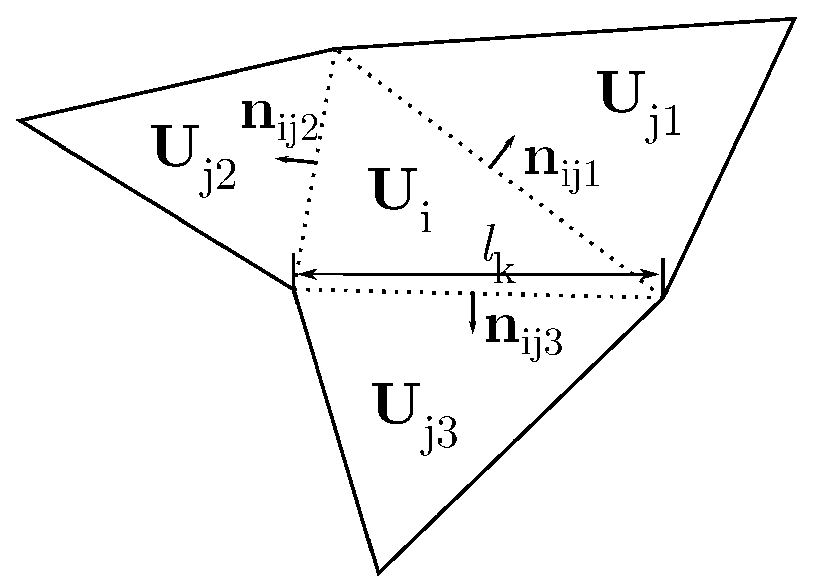
where ${\Omega }_i$ is the area of cell i, n is the current time level and the number of neighboring cells is 3 because triangular cells are used in this work (see, for example, Figure 3). In addition, the fluxes E are evaluated at cell boundaries:

$${\left(\delta \mathbf{E}\right)}_k={\mathbf{E}}_j-{\mathbf{E}}_i$$

(10)

where ${\mathbf{E}}_j$ is the flux value at cell ${\Omega }_j$, and shares a wall k of length $l_k$ with cell ${\Omega }_i$ with a flux value of ${\mathbf{E}}_i$.

Considering the hyperbolic character of system (7), the Jacobian matrix normal to the flow direction, E, can be defined as:

$${\mathbf{J}}_n=\frac{\partial {\mathbf{E}}_n}{\partial \mathbf{U}}=\frac{\partial (\mathbf{E}·\widehat{\mathbf{n}})}{\partial \mathbf{U}}=\frac{\partial \mathbf{F}}{\partial \mathbf{U}}{n}_x+\frac{\partial \mathbf{G}}{\partial \mathbf{U}}{n}_y$$

(11)

The local value of the Jacobian matrix (11), ${\tilde{\mathbf{J}}}_{nk}$, at wall k is

$${\tilde{\mathbf{J}}}_{nk}={\tilde{\mathbf{P}}}_k{\tilde{\mathsf{\Lambda }}}_k{\tilde{\mathbf{P}}}_k^{-1}$$

(12)

where ${\tilde{\mathsf{\Lambda }}}_k$ is the diagonal matrix whose non-zero elements are the eigenvalues of the system ${\tilde{\lambda }}^m$, and ${\tilde{\mathbf{P}}}^m$ is the matrix containing the eigenvectors of the system ${\tilde{\mathbf{e}}}^m$, providing a matrix with three eigenvalues to the 2D model. The eigenvalues and eigenvectors of the Jacobian matrix are:

$${\tilde{\lambda }}_1=\tilde{\mathbf{u}}·\widehat{n}-\tilde{c},{\tilde{\lambda }}_2=\tilde{\mathbf{u}}·\widehat{n},{\tilde{\lambda }}_3=\tilde{\mathbf{u}}·\widehat{n}+\tilde{c}$$

(13)

$$\widetilde{{\mathbf{e}}_1}=\left(\begin{array}{c}1\\ \tilde{u}-\tilde{c}{n}_x\\ \tilde{v}-\tilde{c}{n}_y\end{array}\right),\widetilde{{\mathbf{e}}_2}=\left(\begin{array}{c}0\\ -\tilde{c}{n}_y\\ \tilde{c}{n}_x\end{array}\right),\widetilde{{\mathbf{e}}_3}=\left(\begin{array}{c}1\\ \tilde{u}+\tilde{c}{n}_x\\ \tilde{v}+\tilde{c}{n}_y\end{array}\right)$$

(14)

where $\tilde{\mathbf{u}}·\widehat{n}=\tilde{u}{n}_x+\tilde{v}{n}_y$ and $\tilde{c}$ is the celerity of the infinitesimal surface deformation waves. The tilde variables represent an average state at each cell edge. Therefore, starting from the expression (9), and using the eigenvalues and eigenvectors of the Jacobian matrix, an updated expression at cell i is obtained:

$${\mathbf{U}}_i^{n+1}={\mathbf{U}}_i^n-\frac{\Delta t}{{\Omega }_i}\sum _{k=1}^3\sum _{m=1}^3{\left[{\left(\tilde{\lambda }-\tilde{\gamma }\tilde{\mathbf{e}}\right)}_k^m{l}_k\right]}^n$$

(15)

The time step $\Delta t$ is calculated dynamically throughout the simulation by:

$$\Delta t=\mathrm{CFL}\underset{k,m}{\min }\left(\frac{\delta x_k}{{\tilde{\lambda }}_k^m}\right)$$

(16)

with $0<\mathrm{CFL}\le 1$ to guarantee stability in the numerical scheme, where CFL is the Courant–Friedrichs–Lewy number [47] and

$$\delta x_k=\min ({\chi }_i,{\chi }_j)$$

(17)

where

$${\chi }_i=\frac{{\Omega }_i}{\underset{k}{\max }{l}_k}$$

(18)

Equation (15) is only solved in those cells where water is present and the flooded boundary is not regulated but advances according to the flow dynamics. The method is well designed to deal with this type of calculation ensuring accurate and robust results.

The time step depends, on one hand, on the dynamics of the problem to be solved through ${\tilde{\lambda }}_k^m$ and, on the other hand, on the cell size chosen for the computational grid, given by $l_k$. Therefore, from (16), (17) and (18), it becomes clear that increasing the refinement of the computational grid leads to smaller time steps, and therefore a higher computational cost. For this reason, an unstructured mesh is used, in order not to restrict either the accuracy of the results with a very coarse mesh over the whole domain or the time step $\Delta t$ with a very fine mesh [28].

3. Study Case and Model Setup

3.1. Study Case

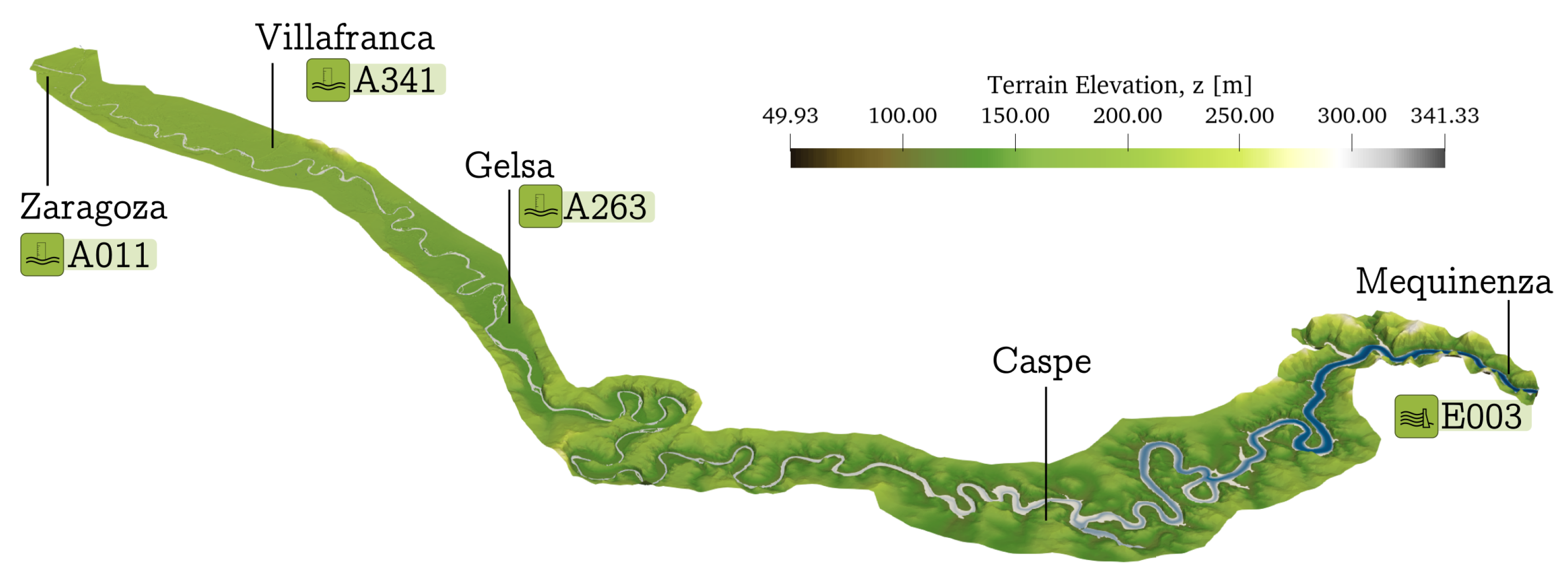
The studied reach of the Ebro River is located between the city of Zaragoza and the Mequinenza Dam. It is more than 200 km long and covers 722 ${\mathrm{km}}^2$ of surface area. Along the river there are a few gauging stations managed by the Ebro River Authority (CHE, www.chebro.es, accessed on 1 March 2023), where the evolution of the flow and surface level are continuously (fortnightly) recorded. Their locations are represented in Figure 4.

The area is continuously suffering from the damage provoked by these events, which have even flooded the A-1107 motorway and collapsed the regional highway (ARA-1) in Villafranca de Ebro (www.heraldo.es/noticias/aragon/2018/04/12/crecidas-del-ebro-las-ultimas-riadas-aragon-1234800-300.html, accessed on 1 March 2023) during the 2015 event (see Figure 1). In addition, it is an area of great importance due to the presence of the Mequinenza reservoir, which runs along about 75 km of the river, and the regulation of its dam. The first 25 km of the studied reach is characterized by meanders and associated with important inundation areas. The final part, on the other hand, is characterized by the reservoir vessel where water is practically at rest.

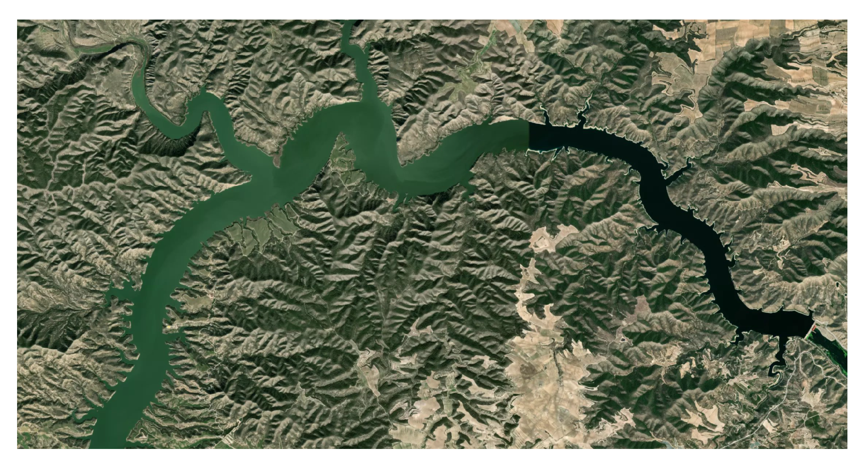
The Mequinenza reservoir, whose satellite view can be seen in Figure 5, covers a surface area of approximately 7540 hectares, with a maximum capacity of 1530 ${\mathrm{hm}}^3$ when the surface level is 121 m.

The Mequinenza dam (see Figure 6) has a crest height of 124 m and a single spillway with six gates located at an elevation of 106.5 m whose discharge limit is 11,000 ${\mathrm{m}}^3/\mathrm{s}$. Data on the reservoir and dam were provided by the Ebro River Authority. The gates at the spillway are used to regulate the volume of water in the reservoir for various purposes, but mainly to control floods and guarantee hydroelectric generation.

3.2. Computational Model Setup

The configuration of the computational model is based on the following parts:

1.

A digital terrain model (DTM);

2.

a surface roughness map;

3.

The creation of a triangular mesh;

4.

Boundary conditions and initial conditions.

3.2.1. Topography: DTM

A raster digital terrain model with a resolution of $5\times 5$ m provided by the IGN (http://centrodedescargas.cnig.es/CentroDescargas/locale?request_locale=en, accessed on 1 March 2023) and obtained by interpolating data from flights with LIDAR sensors in 2010 was used as a base. However, the used data do not contain a reliable representation of the riverbed. Thus, this DTM is used only for floodplains, where a proper representation of the terrain can be found, as seen Figure 7, while complementary information from measured cross-sections is used to reconstruct the river bed, since the LIDAR provides a uniform free surface at the river, as seen in Figure 7.

Reconstruction of the Riverbed from Sástago

To achieve a reliable riverbed, cross-sections of the river are taken at the end of the Osera-Sástago DTM. These cross-sections, which are groups of coordinates $(x,y,z)$, are duplicated along the riverbed up to the Chiprana area. Afterwards, the elevation of the copied sections is corrected, since the terrain through which the river flows descends in altitude. To do this, two points are taken, one at the beginning of the part to be reconstructed and the other at the end. The difference between their elevations is calculated, and the distance that separates them is a straight line. The quotient of these two values is an average slope in the river segment, so that the elevation of each of the sections can be recalculated:

$$z_{ij}=z_{1j}+m\sqrt{{(x_{ij}-x_{1j})}^2+{(y_{ij}-y_{1j})}^2}$$

(19)

where the index i denotes the section number and the index j denotes the point within each section. m denotes the average slope. This methodology is followed from Sástago to the Mequinenza reservoir, where, since there are no sections to start from, it cannot be used.

Reconstruction of the Reservoir

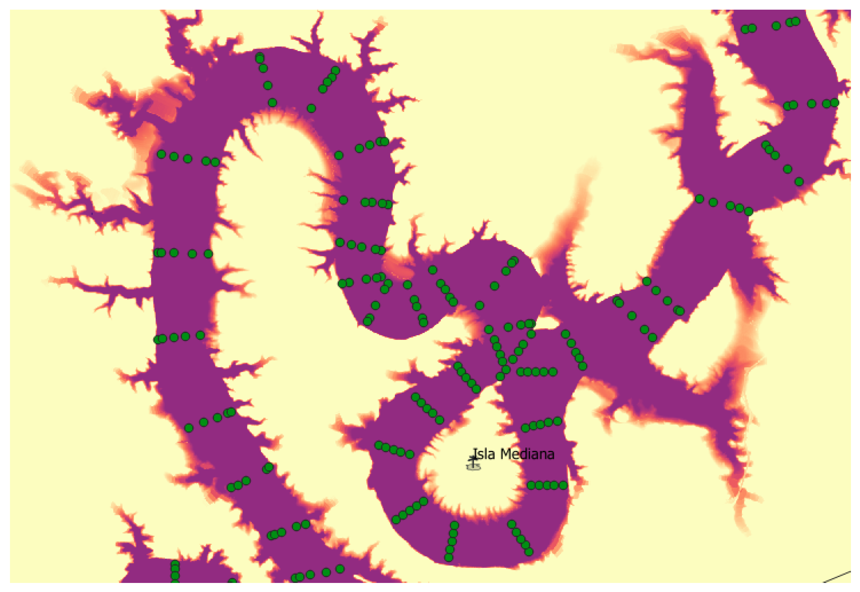
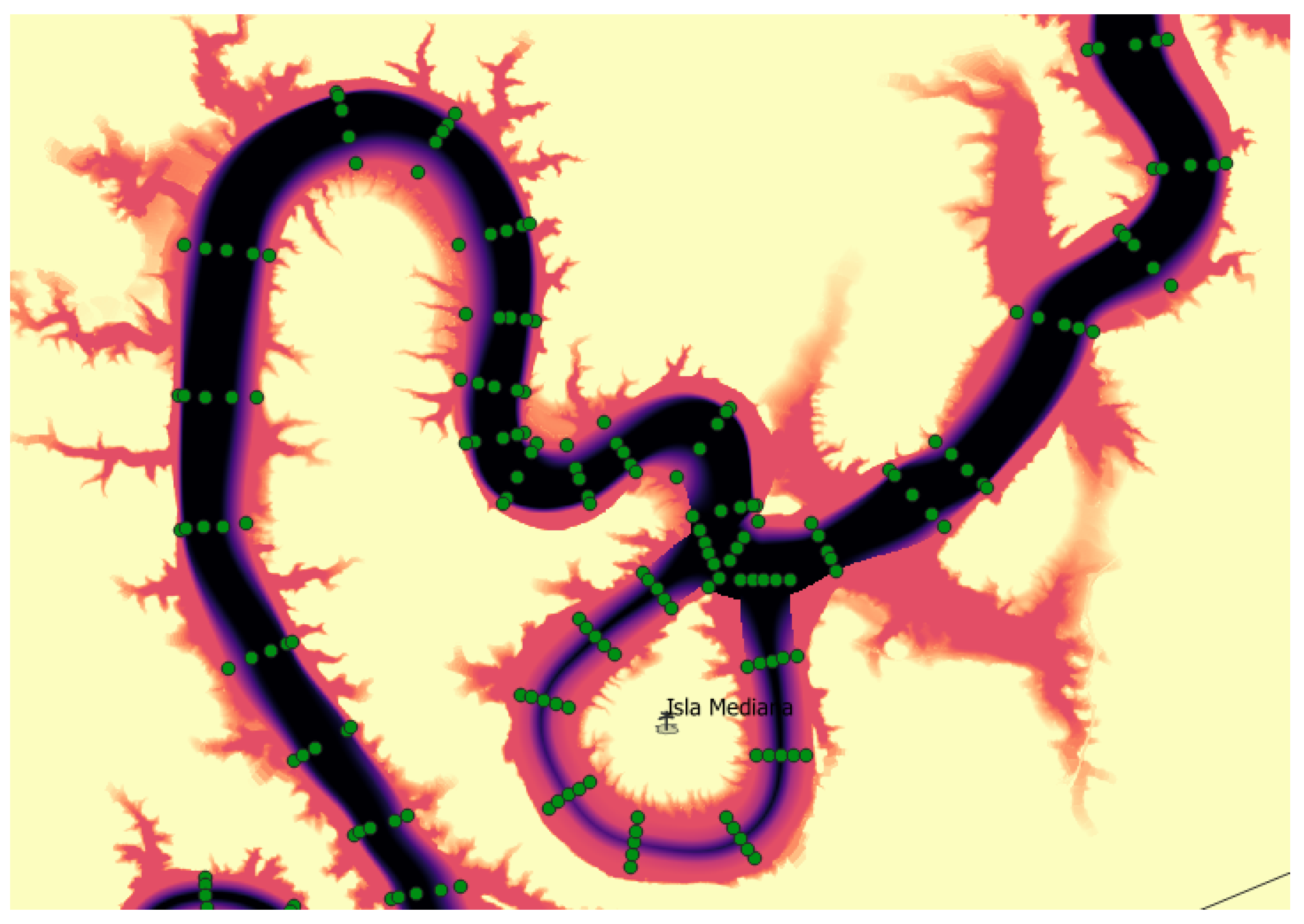
River cross-sections cannot be used to reconstruct the bottom of the reservoir. Therefore, to incorporate that information to the global DTM, geo-referenced historical maps prior to the construction of the dam, also available on the IGN website (http://centrodedescargas.cnig.es/CentroDescargas/locale?request_locale=en, accessed on 1 March 2023) were used. Using their contour lines, new cross-sections are obtained formed by groups of five points with coordinates $(x,y,z)$, as shown in the example in Figure 8, which, after interpolation, produces a DTM with the appropriate reservoir bed elevations. Figure 9 shows an image of the historical map of part of the reservoir, comparing it with the current state. The historical topographic map clearly shows how the Ebro riverbed ran under what is now covered by the reservoir.

The center points of each section, which were not placed on grade lines, were corrected using Equation (19). The lowest elevation of the reservoir bottom, $z=60$ m, was taken in the first section next to the dam, and from there, the minimum elevation of each section was raised. An example of the result is shown in Figure 10.

Using the presented strategy, a channel in the reservoir region similar to the one shown in Figure 11 is obtained, containing the information of the interpolated sections shown in Figure 8. By doing this, a new DTM fo the bottom of the reservoir is obtained and can be added to the global DTM.

3.2.2. Surface Roughness Map

Each computational grid cell is associated with a value of the Manning roughness coefficient, n, which is assigned from a terrain roughness raster map provided by CHE. This map covers the potential floodplain from Zaragoza to Escatrón, where the reservoir starts and the dynamics are not as affected by roughness. Thus, the region covered by the Mequinenza reservoir has a simpler roughness distribution reconstructed following the criteria in the literature [44,48,49]. This distribution is shown in

Table 1. Manning’s coefficient for different types of soil.

Type of Soil	Manning’s Coefficient
Farm land	0.028
Riverbed	0.035
Urban area	0.05
River island	0.06

, and the whole distribution map can be seen in Figure 12.

3.2.3. Meshing

The numerical simulation is based on the discretization of the terrain into cells that form the so-called computational grid. Relevant magnitudes are associated with each of its cells during the simulation, such as bed elevation, water depth or velocity. The computational mesh has a triangular geometry and is spatially adaptive, i.e., the cell size varies in space. The riverbed, the adjacent levees and, in general, all the areas to be represented in detail require a much finer mesh. Less relevant areas or areas with no abrupt changes in elevation can be discretized with larger cell sizes. Figure 13 shows an example of this, where it can be seen that the cells close to the channel have smaller sizes than those of the fields with more or less uniform elevation. In addition, a greater refinement of the mesh is also observed at the levees.

3.2.4. Initial Condition

In river problems, the initial and boundary conditions are of great importance. In order to perform a flooding event simulation, the initial condition must correspond to the steady state state of the river flow before the flood event occurs. For this reason, the initial condition comes from the convergence of the model to a steady flow condition, where the entire river flows with a constant flow of the same value as the discharge at the initial instant of the flood.

3.3. Boundary Conditions

The boundary conditions provide information about how the flow enters and leaves the domain. For the river inflow, the commonly used rating curve boundary condition is applied, i.e., a time variation in discharge at the inlet section of the reach, provided by the gauging station. On the other hand, for the downstream boundary conditions, river simulations typically use a gauging curve. However, the domain under study ends at the Mequinenza dam, so it is necessary to study the most appropriate outflow boundary conditions.

3.3.1. Upstream Boundary Conditions

In the present case, there are inlet sections: the main channel of the Ebro river and the mouths of two tributary rivers (the Gallego River and the Huerva River). A hydrograph-type boundary condition is imposed for all of them. The temporal evolution of the flow imposed in each of the regions is obtained from data provided by CHE at gauging points.

3.3.2. Downstream Boundary Conditions

The boundary conditions considered to model the behavior of the dam are detailed below.

Time-Dependent Level

Considering that the flow is almost at rest when it reaches the reservoir, it can be considered that the level in this region is practically uniform and constant [50]. The way to use this boundary condition in our case will be to impose a constant downstream level throughout the simulation, the value of which will depend on the dimensions of the flood event under study.

Dam Spillway Condition

A weir boundary condition is implemented in this work as a function, $Q_{out}=f\left(H\right)$, to model the dam outflow [51]. Considering certain simplifications, the outflow of a trapezoidal weir follows the expression:

$$Q_{out}=\frac{2}{3}\sqrt{2g}{C}_{d}b{H}_w^{3/2}+\frac{8}{15}\sqrt{2g}tan(\alpha /2)C_d{H}_w^{5/2}$$

(20)

where $H_w=H-h_{Crest}$ is the thickness of the sheet of water above the weir crest $h_{Crest}$; H is the level of the free surface ($H=h+z_b$); $\alpha$ is twice the angle that the lateral sides of the trapezoid make with the vertical; b is the width of the minor base of the trapezoid (see Figure 14); and $C_d=0.611$ [52]. Taking into account the shape of the gates of the Mequinenza dam (see Figure 6), the latter case will be imposed on the output of our problem. In this work, the spillway law is applied to the dam boundary condition as a generic discharge law.

Depending on the value of $H_w$, different outflows through the spillway will be obtained. When the level in the cross-section in contact with the weir is below the crest height, there will be a zero outflow ($H_w\le 0$), while if the level is above ($H_w>0$) the crest height, the outflow will follow the expression (20). Thus, the flow function $Q_{out}=f\left(H\right)$ through the weir is defined as follows:

$$Q_{out}=\left\{\begin{array}{c}{\displaystyle 0\mathrm{if}{H}_w\le 0}\hfill \\ {\displaystyle \frac{2}{3}\sqrt{2g}{C}_{d}b{H}_w^{3/2}\mathrm{if}{H}_w>0}\hfill \end{array}\right.$$

(21)

4. Calibration and Optimization of the Computational Mesh

Although the numerical model used has been validated on numerous occasions and in different domains [20,53], each model configuration requires a calibration process to adjust parameters and correct data that may contain errors. Moreover, even if the model has been calibrated and validated, this does not mean that it is optimal, leading to high computational consumption if the discretization is excessively fine. Therefore, the configuration of the model must be optimized to reduce computational consumption as much as possible.

4.1. Calibration of Mesh Refinement

In this work, an unstructured triangular mesh is used with the advantage of being able to adapt to the topography. This mesh contains smaller cell sizes in those areas with a need for detail, while coarser cells are used in areas where there are few or no relevant terrain irregularities.

Each floodplain has its own topographical particularities that may be relevant not only because of their geometrical characteristics, but also because of the effect they usually have on flooding. There are always overtopped river banks in the first instants of a flood, the modeling of which may have a lower impact than other more distant levees that retain water for long periods of time until they are over passed by water. The detection of these structures is crucial for a correct modeling of the terrain through refinement.

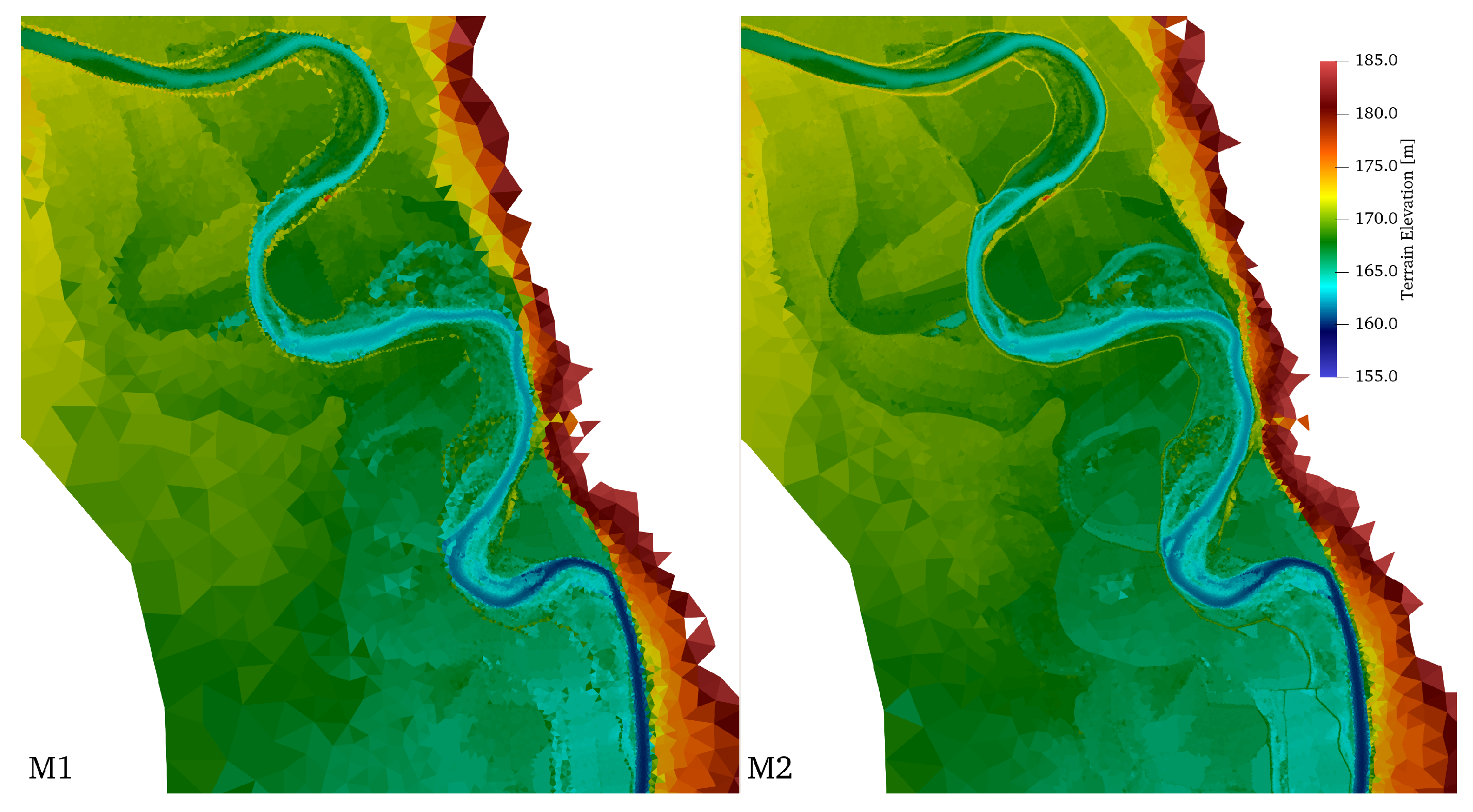
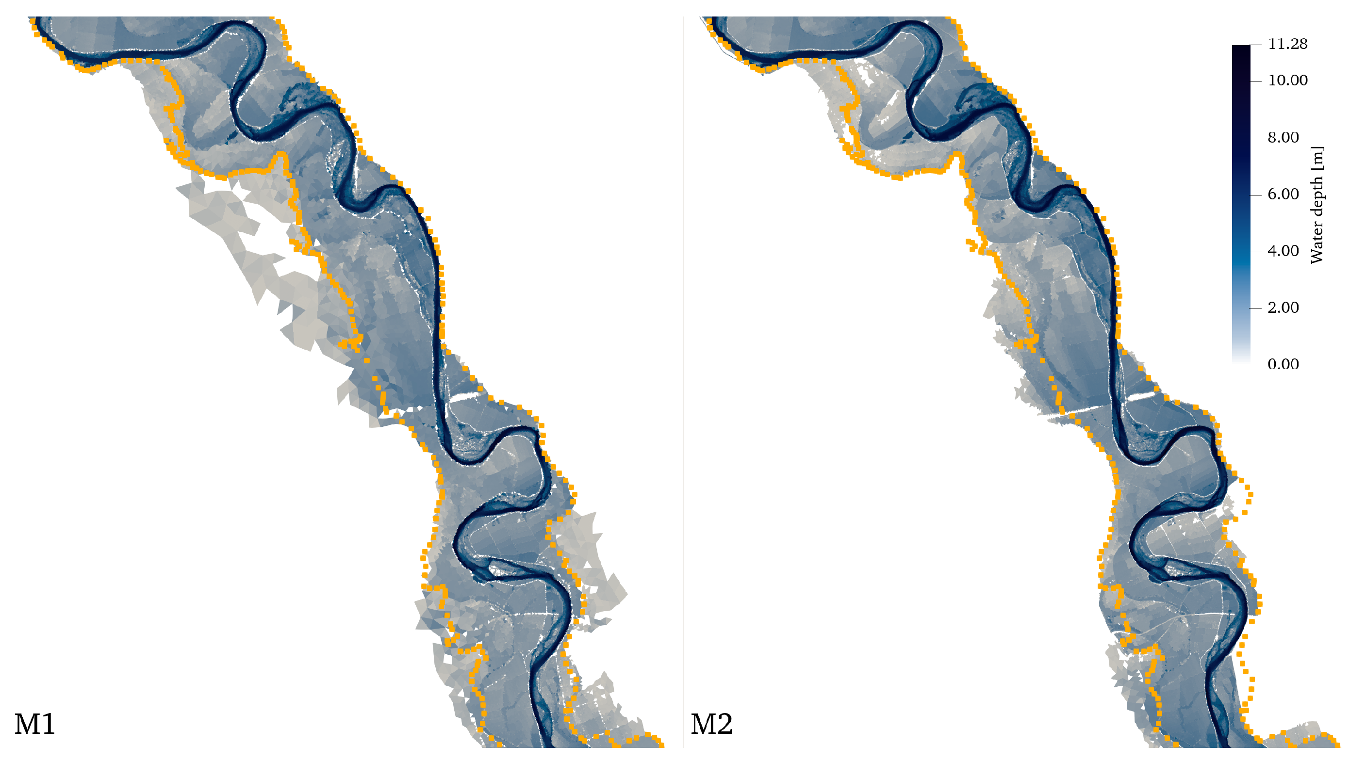
In order to choose the most appropriate mesh, satellite observations of the flood extension are used. By comparing the flooded areas provided by the different computational meshes, sensible zones where refinement was needed were detected. Thus, the cell size distribution of the preliminary mesh, M1, was modified, leading to a refined mesh, M2. The differences in resolution between the meshes are shown in Figure 15, where it can be seen that in M1, some of the floodplain levees are not well represented. This results in different flood extensions that can be seen in Figure 16, where the water depth for a certain time is represented. Finally, in the same figure, those areas provided by the two different meshes are compared to the observed flood envelope points. The preliminary mesh does not retain the water as it should because of the coarse representation of the floodplain irregularities.

To carry out this analysis, the 2018 discharge evolution was used as the inlet boundary condition. As the reservoir has no influence in the flood prone area upstream, a simple constant level is set to the reservoir as the downstream boundary condition.

In

Table 2. Summary of the preliminary mesh and the refined mesh.

Mesh	Number of Cells	Computational Cost (hours)
Preliminary mesh M1	351,799	9.52
Refined mesh M2	949,445	23.80

, some data related to the meshes and their performance can be seen. In view of these results, it can be concluded that, although M2 provides more accurate results, its computational cost is unfeasible. For this reason, a second optimization step was carried out and is detailed in next subsection.

4.2. Optimization

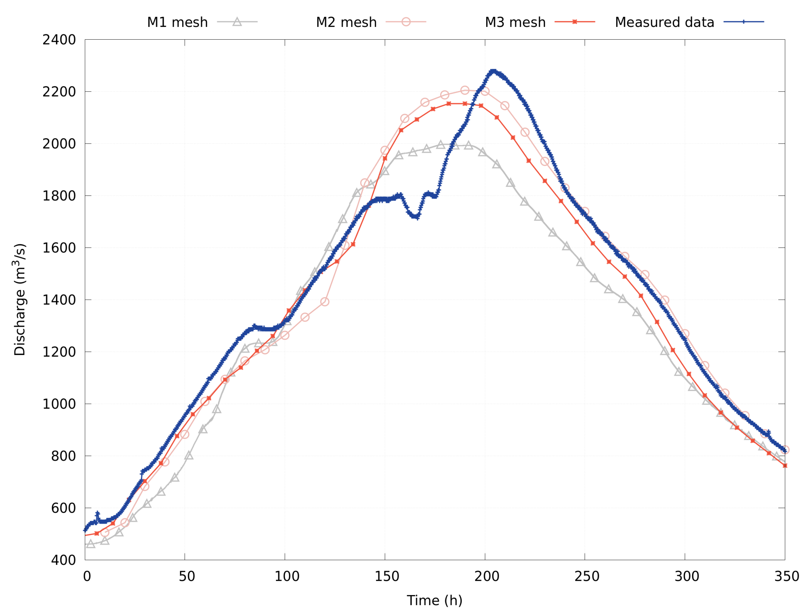
When the mesh is calibrated to refine the results and provide more accurate results, optimization should be performed to reduce the computational consumption without reducing the accuracy of the results. In this work, the optimization of the model was carried out by using internal boundary conditions that allow modeling some hydraulic structures of the channel, such as dikes and motes, without the need for very fine computational meshes [34,54]. In this way, a mesh with a smaller number of cells, M3 mesh, was obtained, with a consequent reduction in computational consumption. The validation of the optimization of the model is carried out by simulating the historical flood event of 2018 and the comparison in the Gelsa gauging station (A263). The results of water level and discharge temporal evolution are shown in Figure 17 and Figure 18, where it can be seen that M1 is much less accurate than M2 and M3, and these two are similar, although M3 is somewhat less accurate than M2. However, this loss of accuracy is justified by the reduction in computational consumption obtained, going from 23.80 h with mesh M2 to 12.48 h with mesh M3, as can be seen in

Table 3. Summary of the calibrated mesh and the optimized mesh.

Mesh	Number of Cells	Computational Cost (hours)
Refined mesh M2	949,445	23.80
Optimized mesh M3	633,216	12.48

. Moreover,

Table 4. Summary of the RMSE of the discharge for the three meshes.

Mesh	RMSE
Preliminary mesh M1	164.65
Refined mesh M2	119.62
Optimized mesh M3	120.24

shows the Root Mean Square Error (RMSE) of the discharge values to demonstrate how accurate each mesh is. The Root Mean Square Error is calculated by the following equation [55]:

$$\mathrm{RMSE}=\sqrt{\frac{{\sum }_{n=1}^N{(x_{f,n}-x_{o,n})}^2}{N}}$$

(22)

where $x_{f,n}$ is the simulated value at time n, $x_{o,n}$ is the measured value at time n and N is the number of measures at a point. Table 4 shows that the accuracy of M1 is lower than M2 and M3, and these two offer a very similar accuracy.

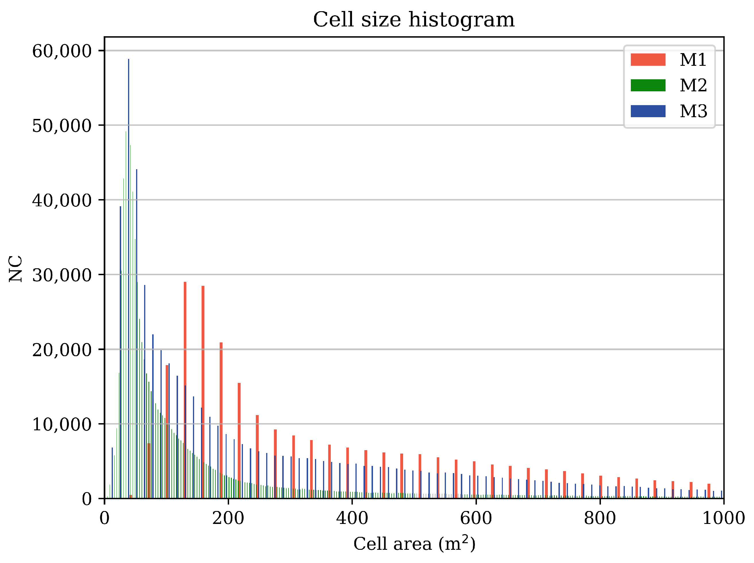
Finally, to provide information on the cell size distribution of the meshes, Figure 19 shows the cell area distribution for each of the analysed meshes (M1, M2 and M3). As the three meshes share the maximum cell size, the x-axis of the figure is bound to 1000 m${}^2$, with the purpose of focusing on the refinement distribution. The M1 mesh contains less refined elements than the other two, with only small cells in the river bed area. The most refined mesh, M2, has a higher concentration of small cells, as the refinement affects not only the river bed but also the levees in the floodplains. Finally, the figure shows how the optimized mesh, M3, is in the middle of the two previously mentioned distributions. The use of an internal boundary condition allows a coarser mesh in the floodplains without loosing accuracy.

5. Numerical Results

A relevant historical event of flooding of the Ebro River which occurred in 2018 was simulated with both analysed downstream boundary conditions: the constant level and the dam model.

2018 Event

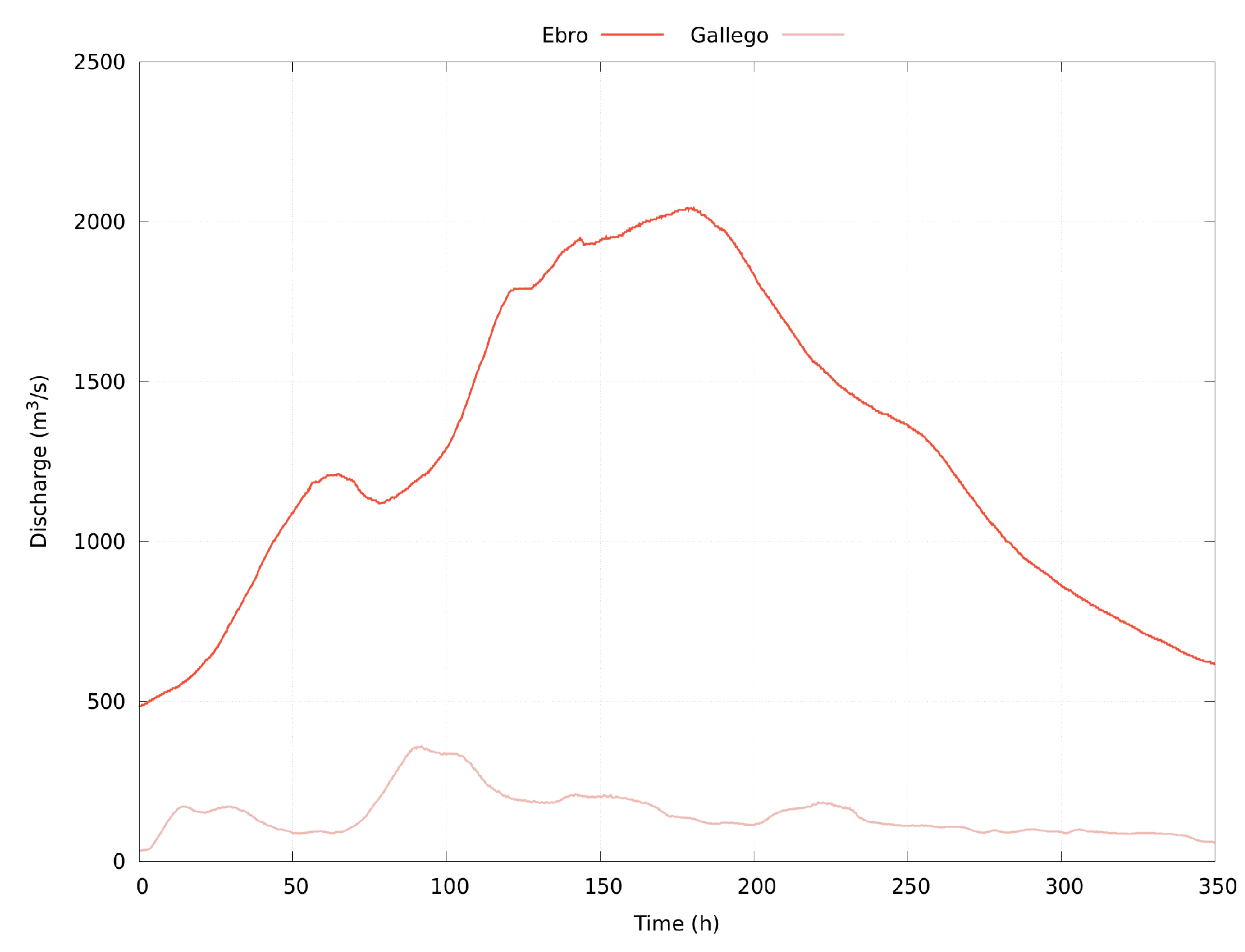
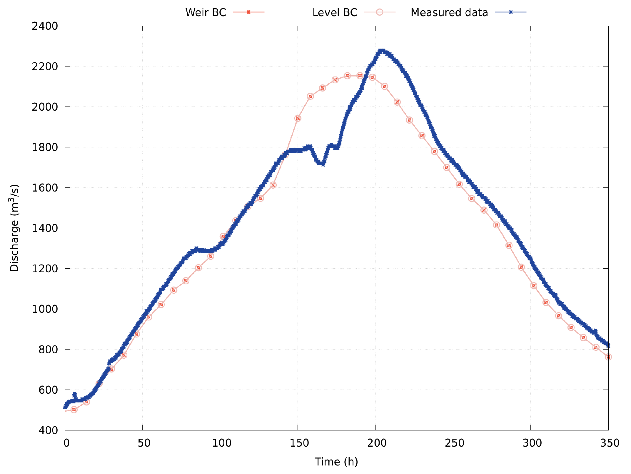
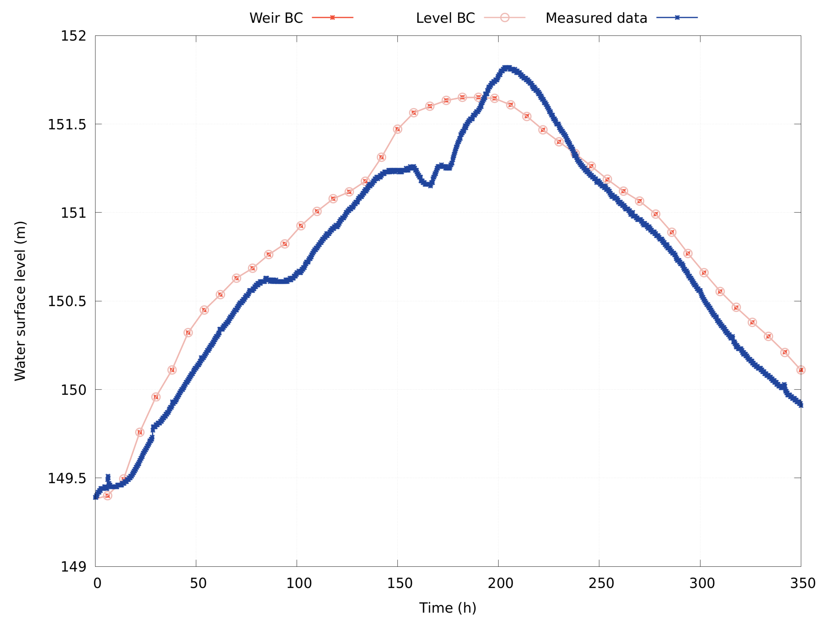
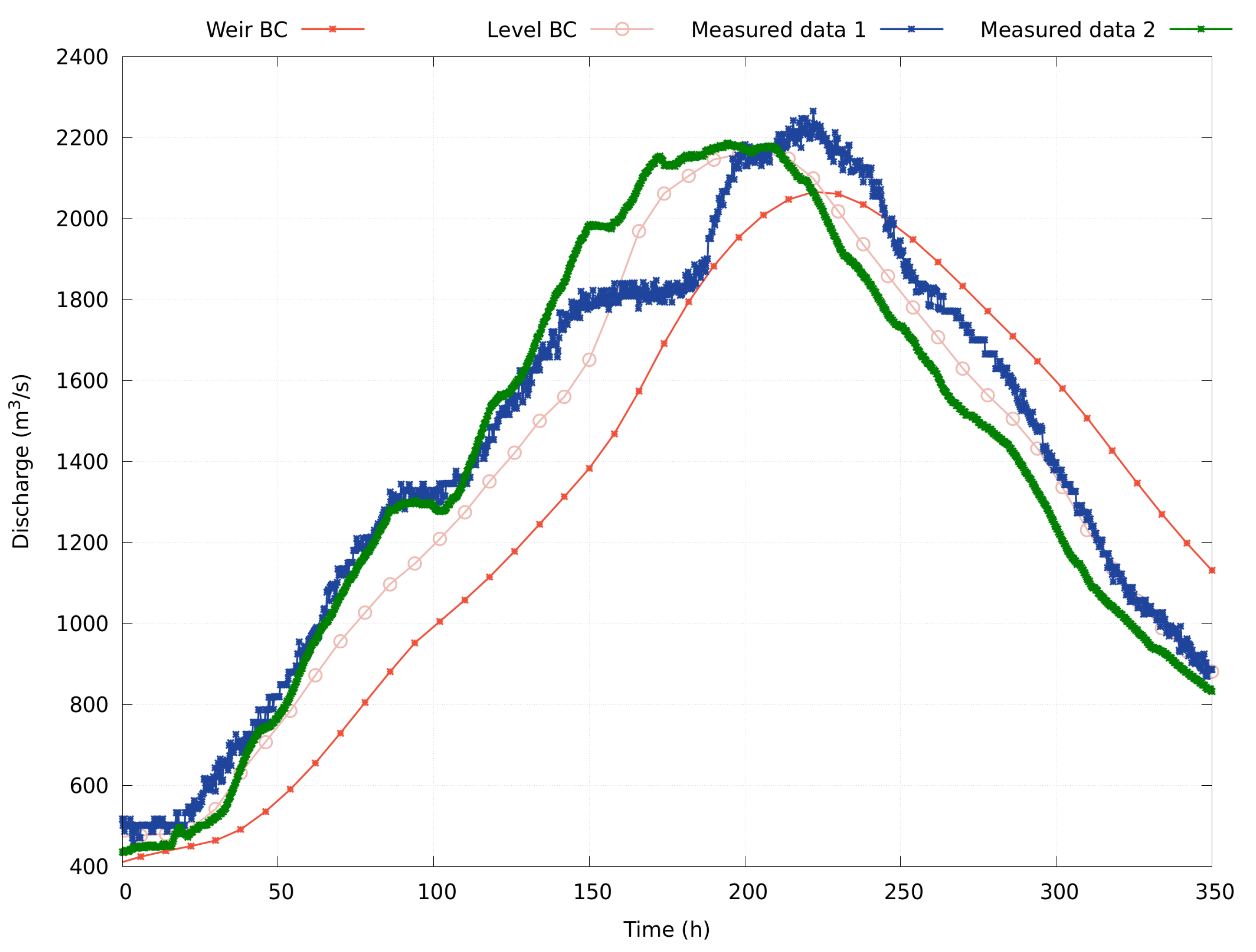
The 2018 inlet hydrograph (see Figure 20), obtained from the Zaragoza gauging station (A011), is set as the upstream boundary condition. As an initial condition, a steady flow with a discharge value that coincides with the initial discharge of the inflow hydrograph is established. A comparison between numerical results and real observation was performed using data from the Gelsa gauging station (A263) (Figure 21 and Figure 22) and the Mequinenza gauging station (E003) (Figure 23 and Figure 24). The results show that at the Gelsa gauging station, both boundary conditions provide the same results since the reservoir does not affect upstream areas such as Gelsa (see Figure 4), as the flow regime is very different from the reservoir in the first half of the studied reach, as can be seen in Figure 21 and Figure 22. At the Mequinenza gauging station, the constant level boundary condition provides a discharge temporal evolution more similar to the actual data than that given by the weir boundary condition (see Figure 23). However, the water level temporal evolution provided by the weir boundary condition is much more realistic than the results from the constant level boundary condition, which cannot represent the temporal evolution of this value, as can be seen in Figure 24.

6. Conclusions

In this work, a finite volume numerical model, well designed for the resolution of unsteady 2D SWE on flexible and adpatative triangular meshes, is used for the simulation of flood events in a specific region of the Ebro River (Spain). This region, which contains a very unique reservoir that changes the river dynamics, presents a challenge for the model regarding dam modeling. For this reason, this work has been able not only to prove the good performance of the model in a particular region, but also to explore new strategies for dam simulations.

First, this study highlights the importance of the choice of computational model. This implies the calibration and optimization of the computational mesh that is first transformed from a coarse to a refined mesh, showing the importance of adaptive meshes and the proper refinement at relevant topography points. From this calibration, it can be concluded that the discretization in certain areas, such as the limits of riverbeds, is crucial to obtain accurate results. However, this produces a very fine mesh with a high number of cells at a high computational cost.

The application to the simulation of flood events in a reach of the Ebro river highlights that the use of real data introduces some uncertainties related with coarse discretization of the terrain measurements, non-detailed characterization of bed roughness, spurious points on the discharge time series and other problems that may provoke errors in the results regardless of the numerical scheme. Hence, a calibration processes must be carried out. An optimal computational mesh has been generated and calibrated for the 2018 flooding event in the Ebro River. Additionally, although real test cases introduce some errors due to the lack of available data, the model is still able to provide very good results. Finally, the benefits of an accurate and fast numerical method are not only desirable for flood prediction, but also the generation of an appropriate computational mesh involving internal boundary conditions. This strategy provides results with enough accuracy, allowing the use of a coarser mesh where the small loss of accuracy obtained is justified by the 12 h of computational savings. These strategies, together with an adequate representation of land use maps, are demonstrated to be necessary in order to carry out computations leading to accurate numerical results.

The historical event was simulated using two different downstream boundary conditions at the Mequinenza dam location. The predictions of discharge and water level at the gauging locations improve when the outlet boundary condition is expressed as a discharge rating curve. This work has highlighted the need for the modeling of hydraulic structures integrated within simulation models instead of simpler boundary conditions. It is worth noting that the downstream boundary condition has no influence on the first half of the river reach, where the cross-sections are shallow and well connected to the floodplain; however, in the second half of the reach, dominated by the long reservoir, a weir-type boundary condition should be used if the temporal evolution of the level is of interest, thus obtaining more realistic results. At this point, it should be noted that this work highlights this need, but opens it up to improvements in terms of dam modeling, where more complex discharge laws could be used and combined to represent bottom spillways, gates and other hydraulic structures.

The numerical results obtained have been presented and compared with measurements. It should be emphasized that the use of HPC technologies is vital when carrying out simulations with large domains and long event durations. In this work, the results for the Ebro River, containing a large domain and great number of computational cells, were obtained using a GPU-parallelized well-balanced upwind numerical scheme which simulates a hydrograph of 14.5 days in a little more than 12 h with a GPU NVIDIA GeForce RTX 3070. Thus, it has been made feasible to reproduce such events on a real-time basis.

References

1. Ripple, W.J.; Wolf, C.; Newsome, T.M.; Barnard, P.; Moomaw, W.R. World Scientists’ Warning of a Climate Emergency. BioScience 2020, 70, 8–12. [Google Scholar] [CrossRef]
2. Wallemacq, P.; Herden, C.; House, R. The Human Cost of Natural Disasters 2015: A Global Perspective; Technical Report; Centre for Research on the Epidemiology of Disasters: Brussels, Belgium, 2015. [Google Scholar]
3. Subdirección General de Prevención, Planificación y Emergencias. Fallecidos por riesgos naturales en España en 2019. 2020. Available online: https://www.proteccioncivil.es/documents/20121/64522/FALLECIMIENTOS+POR+RIESGOS+NATURALES+2019.pdf/ace258bb-e6f2-344b-d056-2fae84dc089c?t=1608632325113 (accessed on 1 February 2023).
4. Hu, H.; Yang, H.; Wen, J.; Zhang, M.; Wu, Y. An Integrated Model of Pluvial Flood Risk and Adaptation Measure Evaluation in Shanghai City. Water 2023, 15, 602. [Google Scholar] [CrossRef]
5. Thielen, J.; Bartholmes, J.; Ramos, M.H.; de Roo, A. The European Flood Alert System—Part 1: Concept and development. Hydrol. Earth Syst. Sci. 2009, 13, 125–140. [Google Scholar] [CrossRef]
6. Knijff, J.M.V.D.; Younis, J.; Roo, A.P.J.D. LISFLOOD: A GISbased distributed model for river basin scale water balance and flood simulation. Int. J. Geogr. Inf. Sci. 2010, 24, 189–212. [Google Scholar] [CrossRef]
7. GebreEgziabher, M.; Demissie, Y. Modeling Urban Flood Inundation and Recession Impacted by Manholes. Water 2020, 12, 1160. [Google Scholar] [CrossRef]
8. Chen, J.; Hill, A.A.; Urbano, L.D. A GIS-based model for urban flood inundation. J. Hydrol. 2009, 373, 184–192. [Google Scholar] [CrossRef]
9. Ghansah, B.; Nyamekye, C.; Owusu, S.; Agyapong, E. Mapping flood prone and Hazards Areas in rural landscape using landsat images and random forest classification: Case study of Nasia watershed in Ghana. Civ. Environ. Eng. 2021, 8, 1923384. [Google Scholar] [CrossRef]
10. Olcina, J.; Sauri, D.; Hernández, M.; Ribas, A. Flood policy in Spain: A review for the period 1983–2013. Disaster Prevent. Manag. 2016, 25, 41–58. [Google Scholar] [CrossRef]
11. European Parliament 2007 Directive 2007/60/EC of the European Parliament and of the Council of 23 October 2007 on the Assessment and Management of Flood Risks. EU Directive. 2007. Available online: https://eur-lex.europa.eu/legal-content/EN/TXT/?uri=celex:32007L0060 (accessed on 1 February 2023).
12. European Environment Agency. The European Environment—State and Outlook 2020; EEA: Copenhagen, Denmark, 2019. [Google Scholar]
13. Vacondio, R.; Aureli, F.; Ferrari, A.; Mignosa, P.; Palù, A. Simulation of the January 2014 flood on the Secchia River using a fast and high-resolution 2D parallel shallow-water numerical scheme. Nat. Hazards 2016, 80, 1–23. [Google Scholar] [CrossRef]
14. Horritt, M.S.; Bates, P.D. Evaluation of 1D and 2D numerical models for predicting river flood inundation. J. Hydrol 2002, 268, 89–99. [Google Scholar] [CrossRef]
15. Sampson, C.C.; Smith, A.M.; Bates, P.D.; Neall, J.C.; Alfieri, L.; Freer, J.E. A high-resolution global flood hazard model. Water Resour. Res. 2015, 51, 7358–7381. [Google Scholar] [CrossRef]
16. Lacasta, A.; Juez, C.; Murillo, J.; García-Navarro, P. An efficient solution for hazardous geophysical flows simulation using GPUs. Comput. Geosci. 2015, 78, 63–72. [Google Scholar] [CrossRef]
17. Kalyanapu, A.J.; Shankar, S.; Pardyjak, E.R.; Judi, D.R.; Burian, S.J. Assessment of GPU computational enhancement to a 2D flood model. Environ. Model. Softw. 2011, 26, 1009–1016. [Google Scholar] [CrossRef]
18. Briganti, R.; Dodd, N. Shoreline motion in nonlinear shallow water coastal models. Coast. Eng. 2009, 56, 495–505. [Google Scholar] [CrossRef]
19. Hubbard, M.E.; Dodd, N. A 2D numerical model of wave run-up and overtopping. Coast. Eng. 2002, 47, 1–26. [Google Scholar] [CrossRef]
20. Echeverribar, I.; Morales-Hernández, M.; Brufau, P.; García-Navarro, P. 2D numerical simulation of unsteady flows for large scale floods prediction in real time. Adv. Water Resour. 2019, 134, 103444. [Google Scholar] [CrossRef]
21. Bomers, A.; Schielen, R.M.J.; Hulscher, S.J.M.H. The influence of grid shape and grid size on hydraulic river modelling performance. Environ. Fluid Mech. 2019, 19, 1273–1294. [Google Scholar] [CrossRef]
22. Sanders, B.; Schubert, J.; Detwiler, R. Parbrezo: A parallel, unstructured grid, Godunov type, shallow water code for high resolution flood inundation modeling at the regional scale. Adv. Water Resour. 2010, 33, 1456–1467. [Google Scholar] [CrossRef]
23. Masoero, A.; Claps, P.; Asselman, N.E.M.; Mosselman, E.; Di Baldassarre, G. Reconstruction and analysis of the Po river inundation of 1951. Hydrol. Process. 2013, 27, 1341–1348. [Google Scholar] [CrossRef]
24. Defina, A. Two-dimensional shallow flow equations for partially dry areas. Water Resourc. Res. 2000, 36, 3251–3264. [Google Scholar] [CrossRef]
25. Costabile, P.; Costanzo, C.; Macchione, F. Performances and limitations of the diffusive approximation of the 2-d shallow water equations for flood simulation in urban and rural areas. Appl. Numer. Math. 2017, 116, 141–156. [Google Scholar] [CrossRef]
26. Yoshida, H.; Dittrich, A. 1D unsteady-state flow simulation of a section of the upper Rhine. J. Hydrol. 2002, 269, 79–88. [Google Scholar] [CrossRef]
27. Masood, M.; Takeuchi, K. Assessment of flood hazard, vulnerability and risk of mid-eastern Dhaka using DEM and 1D hydrodynamic model. Nat. Hazards 2012, 61, 757–770. [Google Scholar] [CrossRef]
28. Hu, R.; Fang, F.; Salinas, P.; Pain, C.C.; Sto.Domingo, N.D.; Mark, O. Numerical simulation of floods from multiple sources using an adaptive anisotropic unstructured mesh method. Adv. Water Resour. 2019, 123, 173–188. [Google Scholar] [CrossRef]
29. Noh, S.J.; Lee, J.H.; Lee, S.; Kawaike, K.; Seo, D.J. Hyper-resolution 1D-2D urban flood modelling using LiDAR data and hybrid parallelization. Environ. Modell. Softw. 2018, 103, 131–145. [Google Scholar] [CrossRef]
30. de Almeida, G.A.M.; Bates, P.; Freer, J.E.; Souvignet, M. Improving the stability of a simple formulation of the shallow water equations for 2-D flood modeling. Water Resour. Res. 2012, 48, W05528. [Google Scholar] [CrossRef]
31. Mignot, E.; Paquier, A.; Haider, S. Modeling floods in a dense urban area using 2D shallow water equations. J. Hydrol. 2006, 327, 186–199. [Google Scholar] [CrossRef]
32. Özgen, I.; Zhao, J.; Liang, D.; Hinkelmann, R. Urban flood modeling using shallow water equations with depth-dependent anisotropic porosity. J. Hydrol. 2016, 541, 1165–1184. [Google Scholar] [CrossRef]
33. Sanders, B.F.; Schubert, J.E.; Gallegos, H.A. Integral formulation of shallow-water equations with anisotropic porosity for urban flood modeling. J. Hydrol. 2008, 362, 19–38. [Google Scholar] [CrossRef]
34. Echeverribar, I.; Morales-Hernández, M.; Brufau, P.; García-Navarro, P. Use of internal boundary conditions for levees representation: Application to river flood management. Environ. Fluid. Mech. 2019, 19, 1253–1271. [Google Scholar] [CrossRef]
35. Chow, V.T.; Maidment, D.R.; Mays, L.W. Applied Hydrology; McGraw-Hill: New York, NY, USA, 1988. [Google Scholar]
36. Fiorentini, M.; Orlandini, S. Robust numerical solution of the reservoir routing equation. Adv.Water Resour. 2013, 59, 123–132. [Google Scholar] [CrossRef]
37. Liu, Y.; Yang, W.; Wang, X. Development of a SWAT extension module to simulate riparian wetland hydrologic processes at a watershed scale. Hydrol. Process. 2008, 22, 2901–2915. [Google Scholar] [CrossRef]
38. Dorchies, D.; Thirel, G.; Jay-Allemand, M.; Chauveau, M.; Dehay, F.; Bourgin, P.-Y.; Perrinb, C.; Joste, C.; Rizzolie, J.L.; Demerliac, S.; et al. Climate change impacts on multi-objective reservoir management: Case study on the Seine River basin, France. Int. J. River Basin Manag. 2014, 12, 265–283. [Google Scholar] [CrossRef]
39. Cohen Liechti, T.; Matos, J.P.; Ferràs Segura, D.; Boillat, J.-L.; Schleiss, A.J. Hydrological modelling of the Zambezi River Basin taking into account floodplain behaviour by a modified reservoir approach. Int. J. River Basin Manag. 2014, 12, 29–41. [Google Scholar] [CrossRef]
40. Mohammad, M.E.; Al-Ansari, N.; Issa, I.E.; Knutsson, S. Sediment in Mosul Dam reservoir using the HEC-RAS model. Lakes Reserv. Res. Manag. 2016, 21, 235–244. [Google Scholar] [CrossRef]
41. Murillo, J.; García-Navarro, P. Wave Riemann description of friction terms in unsteady shallow flows: Application to water and mud/debris floods. J. Comput. Phys. 2012, 231, 1963–2001. [Google Scholar] [CrossRef]
42. Murillo, J.; García-Navarro, P. Weak solutions for partial differential equations with source terms: Application to the shallow water equations. J. Comput. Phys. 2010, 229, 4237–4368. [Google Scholar] [CrossRef]
43. Cunge, J.; Holly, F.; Verwey, A. Practical Aspects of Computational River Hydraulics; Pitman: London, UK, 1980. [Google Scholar]
44. Arcement, G.; Schneider, V. Guide for Selecting Manning’s Roughness Coefficients for Natural Channels and Flood Plains. In US Geological Survey. Water-Supply Paper; USGS Publications Warehouse: Washington, DC, USA, 1984; Volume 2339. [Google Scholar]
45. Toro, E.F. The Riemann Solver of Roe. In Riemann Solvers and Numerical Methods for Fluid Dynamics; Springer: Berlin/Heidelberg, Germany, 1997; pp. 313–343. [Google Scholar]
46. Morales-Hernández, M.; Petaccia, G.; Brufau, P.; García-Navarro, P. Conservative 1D–2D coupled numerical strategies applied to river flooding: The Tiber (Rome). Appl. Math. Model. 2016, 40, 2087–2105. [Google Scholar] [CrossRef]
47. Leveque, R. Numerical Methods for Conservation Laws Lectures in Mathematics; ETH: Zürich, Switzerland; Birkhuser: Basel, Switzerland, 1992. [Google Scholar]
48. Chow, V.T. Open-Channel Hydraulics, 1st ed.; McGraw-Hill: New York, NY, USA, 1959. [Google Scholar]
49. Palmeri, F.; Silván, F.; Prieto, I.; Balboni, M.; García-Mijangos, I. Manual de Técnicas de Ingeniería Naturalística en Ambito Fluvial; Departamento de Ordenación del Territorio y Medio Ambiente, País Vasco Government: Bilbao, Spain, 2002. [Google Scholar]
50. Fread, D.; Hsu, K. Applicability of Two Simplified Flood Routing Methods: Level-Pool and Muskingum-Cunge. In Proceedings of the ASCE National Hydraulic Engineering Conference, San Francisco, CA, USA, 25–30 July 1993; pp. 1564–1568. [Google Scholar]
51. Sotelo, G. Hidráulica General Vol. 1, 1st ed.; Limusa: Wellington, FL, USA, 2002. [Google Scholar]
52. Henderson, F.M. Open Channel Flow; Macmillan Series in Civil Engineering; McGraw-Hill: New York, NY, USA, 1966. [Google Scholar]
53. Fernández-Pato, J.; Sánchez, A.; García-Navarro, P. Simulación de avenidas mediante un modelo hidráulico/hidrológico distribuido en un tramo urbano del río Ginel (Fuentes de Ebro). Ribagua 2019, 6, 49–62. [Google Scholar] [CrossRef]
54. Morales-Hernández, M.; Murillo, J.; García-Navarro, P. The formulation of internal boundary conditions in unsteady 2D shallow water flows: Application to flood regulation. Water Resour. Res. 2013, 80, 225–232. [Google Scholar]
55. Barnston, A.G. Correspondence among the Correlation, RMSE, and Heidke Forecast Verification Measures; Refinement of the Heidke Score. Wea. Forecast. 1992, 7, 699–709. [Google Scholar] [CrossRef]
Figure 1. Damage produced by a flood event in crops around Zaragoza (Spain): flooding in Pina de Ebro (2015) (a) (Source: EFE) and flooding in Novillas (2018) (b) (Source: Guardia Civil).
Geohazards 04 00009 g001
Figure 2. Location of Spain in Europe (a); location of the Ebro River basin in Spain (b) and location of the computational domain of the study in the basin (c).
Geohazards 04 00009 g002
Figure 3. Diagram of the cells in a two-dimensional case with triangular cells.
Geohazards 04 00009 g003
Figure 4. Representation of the 2D simulation domain of the Ebro River with the most important cities and gauging stations of CHE. The labels correspond to the official names of the gauging stations.
Geohazards 04 00009 g004
Figure 5. Satellite view of the final stretch of the Mequinenza reservoir. [Source: Mapquest].
Geohazards 04 00009 g005
Figure 6. Front view of the Mequinenza dam. [Source: CHE].
Geohazards 04 00009 g006
Figure 7. Raster representation with an elevation scale in meters of Galacho de la Alfranca and its surroundings with a resolution of 5 × 5 m.
Geohazards 04 00009 g007
Figure 8. Examples of the sections used to interpolate the reservoir bed level.
Geohazards 04 00009 g008
Figure 9. Comparison between two maps showing a part of the Mequinenza reservoir. (a) shows the historical topographic map (Source: IGN) and (b) shows the same area photographed today (Source: Google Maps).
Geohazards 04 00009 g009
Figure 10. Comparative images of the DTM raster at the height of the Mequinenza dam. (a) shows the IGN DTM with the reservoir at constant elevation 117.9 m. (b) shows the result of interpolating the sections obtained from the old topographic maps.
Geohazards 04 00009 g010
Figure 11. Example of the result of interpolating the sections shown in Figure 8.
Geohazards 04 00009 g011
Figure 12. Manning coefficient distribution in the domain of the Ebro River.
Geohazards 04 00009 g012
Figure 13. Real satellite view (a) (Source: Google Maps) and the meshing (b) of an area of Ebro River domain.
Geohazards 04 00009 g013
Figure 14. Frontal (a) and side (b) view of the weir boundary condition.
Geohazards 04 00009 g014
Figure 15. Comparison between the first computational mesh, M1 (left), and the refined mesh, M2 (right), in a certain area of the domain.
Geohazards 04 00009 g015
Figure 16. Comparison between the first computational mesh, M1 (left), and the refined mesh, M2 (right), at a certain area of the domain.
Geohazards 04 00009 g016
Figure 17. Discharge temporal evolution comparison between preliminary mesh, M1, refined mesh, M2, and optimized mesh, M3, in Gelsa (A263).
Geohazards 04 00009 g017
Figure 18. Water level temporal evolution comparison between preliminary mesh, M1, refined mesh, M2, and optimized mesh, M3, in Gelsa (A263).
Geohazards 04 00009 g018
Figure 19. Cell size histogram for preliminary mesh, M1; refined mesh, M2; and optimized mesh, M3.
Geohazards 04 00009 g019
Figure 20. Inlet hydrograph for the Ebro River flooding event in 2018 in Zaragoza (A011).
Geohazards 04 00009 g020
Figure 21. Discharge temporal evolution comparison between the models and observations at Gelsa (A263) for the 2018 flooding event.
Geohazards 04 00009 g021
Figure 22. Water level temporal evolution comparison between the models and observations at Gelsa (A263) for the 2018 flooding event.
Geohazards 04 00009 g022
Figure 23. Discharge temporal evolution comparison between the models and observations at Mequinenza (E003) for the 2018 flooding event.
Geohazards 04 00009 g023
Figure 24. Water level temporal evolution comparison between the models and observations at Mequinenza (E003) for the 2018 flooding event.
Geohazards 04 00009 g024