Article

Earthquake Nowcasting with Deep Learning

1
Biocomplexity Institute and Initiative, University of Virginia, Charlottesville, VA 22904, USA
2
Computer Science Department, University of Virginia, Charlottesville, VA 22904, USA
3
Physics and Astronomy and Geology, University of California, Davis, CA 95616, USA
4
Jet Propulsion Laboratory, California Institute of Technology, Pasadena, CA 91109, USA
5
Santa Fe Institute, Santa Fe, NM 87501, USA
6
Luddy School of Informatics, Computing, and Engineering, Indiana University, Bloomington, IN 47408, USA
*
Author to whom correspondence should be addressed.
GeoHazards 2022, 3(2), 199-226; https://doi.org/10.3390/geohazards3020011
Submission received: 24 December 2021 / Revised: 20 March 2022 / Accepted: 2 April 2022 / Published: 15 April 2022

Abstract

:
We review previous approaches to nowcasting earthquakes and introduce new approaches based on deep learning using three distinct models based on recurrent neural networks and transformers. We discuss different choices for observables and measures presenting promising initial results for a region of Southern California from 1950–2020. Earthquake activity is predicted as a function of 0.1-degree spatial bins for time periods varying from two weeks to four years. The overall quality is measured by the Nash Sutcliffe efficiency comparing the deviation of nowcast and observation with the variance over time in each spatial region. The software is available as open source together with the preprocessed data from the USGS.

1. Introduction

Earthquake forecasting is an old but challenging problem with many interesting characteristics. In studying this, we not only hope to shed light on this socioscientific challenge but also lead to new methods based on deep learning that can be applied in other areas. Perhaps the most essential characteristic is the nature of its challenge. Namely, it is unlikely that building a new zettascale supercomputer will accurately simulate quakes and lead to reliable earthquake predictions [1]. As a phase transition in a system with unknown boundary conditions and phenomenological models (as for friction), it is not obvious that earthquakes are the solution of a set of differential equations or that accurate probabilities of large events can be computed. For these reasons, we have recently chosen to focus on earthquake nowcasting [2], which is the estimation of hazard in the present, the immediate past, and the near future.
Earthquake nowcasting is an archetype of data-intensive problems characteristic of the fourth paradigm of scientific discovery [3] in that we suppose that the patterns of previous events hold clues to the future. This is a bit different from other studies where machine learning has been successful. For example, language translation and image recognition are very complicated problems, but one can see the natural patterns from grammar, words, segments, colors, etc., that are clearly but complexly correlated with what we want to discover. Machine learning successfully learns this complex relationship between inputs and predictions [4].
Earthquake nowcasting challenges AI to discover “hidden variables” in a case where their existence is not as clear as in other successes of machine and deep learning. These ideas are illustrated in Figure 1 where we are pursuing the right side data-intensive approach, rather than developing a theoretical model and determining unknown parameters from the data. In this paper, everything is hidden and determined by the data! Data-driven methods avoid the bias of incomplete theories but maybe there is not rich enough data to provide good insights. We partly address this here with a choice of “known inputs” which are natural mathematical expansion functions explained in Section 4.4.
The history of earthquakes is recorded as events detailing the (three-dimensional) position and size of each quake. While we can observe the events themselves, the underlying stress–strain dynamics remain hidden from view. Earthquakes can be binned in space and time to generate geospatial time series corresponding to sequences in time labeled by spatial position (and bin size). This class of problem is prevalent in both science (research) and commercial areas. Perhaps the most intense study of this problem has come from traffic transportation studies with many innovations aimed at ride-hailing, with papers from, for example, the companies Uber and Didi as well as academia [5,6,7,8,9]. However, there are also many medical and Earth/environmental science problems of this type [10,11,12,13,14,15]. This problem class includes cases where there is a significant spatial structure that typically strongly affects nearby space points. In the case of earthquakes, it is known that the events transfer stress from one location to another via stress Greens’ functions, thus interactions are ever-present.
Details of the geometric structure are important, for example, in traffic-related problems where the road network and function of land use define a graph structure relating different spatial points [7,16,17,18]. The problem chosen is termed [19,20] a spatial bag where there is spatial variation but it is not clearly linked to the geometric distance between spatial regions. Earthquakes have obvious coarse grain spatial structure, but local structure comes from faults, and we have not found this useful in the current analysis, meaning that it is therefore in the spatial bag class. Hydrology study of catchments [10,21] is also a spatial bag problem. Different catchments are related by values of static attributes such as aridity, elevation, and the nature of the soil and not directly by geometry.
In the following text, we first review the use of nowcasting and machine learning for earthquakes. Then, we describe the data setup for our analysis including how we compare with the nowcasted predictions. Then, we present the three deep learning methods used in this work with the following section discussing attention and the transformer architecture used in two of the methods. The next section presents nowcasting results from each of these methods and, in the conclusion, we finish with a summary of some open questions in this promising but preliminary area. We hope that the deep learning approach will be more general than previous methods and not require a prior guesswork as to what patterns are important.

2. Introduction to Earthquake Nowcasting

Earthquakes are a clear and present danger to world communities [22], and many earthquake forecasting methods have been proposed to date with little success. A comprehensive recent review is given by ref. [23]. In this paper, we continue the development of a new approach, earthquake nowcasting, using machine learning methods that have recently been developed.
Nowcasting is a term originating from economics, finance, and meteorology. It refers to the process of determining the uncertain state of the economy, markets, or the weather at the “current time” by indirect means. By the “current time” we mean the present, the immediate past, and the very near future. Rundle [24,25] and Donnellan [23,26,27] have applied this idea to seismically active regions, where the goal is to determine the current state of the fault system, and its current level of progress through the earthquake cycle. In our implementation of this idea, we use the global catalog of earthquakes, using “small” earthquakes to determine the level of hazard from “large” earthquakes in the region.
The original method is based on the idea of an earthquake cycle. A specific region and a specific large earthquake magnitude of interest were defined, ensuring that there is enough data to span at least 20 or more large earthquake cycles in the region. An “Earthquake Potential Score” (EPS) was then defined as the cumulative probability distribution P ( n < n ( t ) ) for the current count n ( t ) for the small earthquakes in the region. Physically, the EPS corresponds to an estimate of the level of progress through the earthquake cycle in the defined region at the current time.
In the past, this determination of the state of a regional fault system has focused on trying to estimate the state of stress in the Earth, its relation to the failure strength of the active faults in a region, and the rate of accumulation of tectonic stress. Determining the values of these parameters would allow researchers to estimate the proximity to failure of the faults in the region. This would be an answer to the question of “how far along is the region in the earthquake cycle?”.
An example application of this method is shown in Figure 2. Here, we show the EPS for a region surrounding Los Angeles within a circle of radius 150 km, for earthquakes of magnitude M 6 [27]. The last such earthquake was the Northridge, CA earthquake of 17 January 1994. The green vertical bars represent a histogram of the number of small earthquakes between large earthquakes M 6 in a region 4000 km × 4000 km surrounding Los Angeles. The solid red line is the corresponding cumulative distribution function (CDF). The thin dashed lines represent the 68% confidence bound on the CDF. The red dot represents the number of small earthquakes that have occurred in the region since the Northridge event.
A different but related method uses small earthquake bursts that are strongly clustered in space and time ([24,25]; Figure 3). These include seismic swarms and aftershock sequences. A readily observable property of these events, the radius of gyration (RG), allows us to connect the bursts to the temporal occurrence of the largest M 7 earthquakes in California since 1984. Here, the radius of gyration of a small earthquake burst is a statistical measure of the horizontal size of that burst. It is computed by finding the centroid of the burst and then computing the distribution of other earthquakes in the burst about the centroid. It is similar in concept to computing the moment of inertia, where the “mass” is assumed to be 1 for each small earthquake [24].
In the Southern California earthquake catalog, they identify hundreds of these potentially coherent space–time structures in a region defined by a circle of radius 600 km around Los Angeles. They compute R G for each cluster, then filter them to identify those groups of events with large numbers of events closely clustered in space, which we call “compact” bursts. The basic assumption is that these compact bursts reflect the dynamics associated with large earthquakes.
Once the burst catalog has been filtered, they apply an exponential moving average to construct a time series R G ( t ) for the Southern California region. They observe that the R G ( t ) of these bursts systematically decreases prior to large earthquakes, in a process that they term “radial localization”. The R G ( t ) then rapidly increases during an aftershock sequence, and a new cycle of “radial localization” then begins.
These time series display cycles of recharge and discharge reminiscent of seismic stress accumulation and release in the elastic rebound process. This time series is shown in Figure 3. Vertical red dashed lines represent major earthquakes having magnitudes M 7 , vertical dotted lines represent earthquakes having 6 M 7 . The green horizontal line near the top is a decision threshold DRG(TW) used for an optimal receiver operating characteristic analysis with an alert time of T W = 3 years [23,26].
A similar time series that is based on different correlation metrics has been constructed by Rundle et al. [23,26]. This method uses a new machine learning-based method for nowcasting earthquakes to image the time-dependent earthquake cycle, involving the classification of seismicity into characteristic patterns found by using principal component analysis of regional seismicity ([28,29]). Patterns are found as eigenvectors of the cross-correlation matrix of a collection of seismicity time series in a coarse-grained regional spatial grid (pattern recognition via unsupervised machine learning). Data from 1950–present were used, with magnitudes M 3.29 . The eigenvalues of this matrix represent the relative importance of the various eigenpatterns. Examples of the most prominent eigenvectors are shown in Rundle et al. [23,26,30].
We can now ask whether it might be possible to apply machine learning (ML) techniques to predict future values of the time series. The general method we have used is to divide the data into a training and a test set, with the training period to fix the parameters, and the test set to evaluate the quality of the prediction. There are at least three techniques that we use in the process of evaluating. These are all one-step walk-forward methods in which a set of N previous values { x t , x t 1 , , x t N } are used as the feature vector x. The label y that is assigned for the supervised learning task is the next value of the time series beyond x t , y = x t + 1 .
Once the model is trained, it is evaluated on the test or validation data. There are three methods that we have investigated based on:
  • Random forest classifiers (RFCs) [31];
  • Auto-regressive integrated moving average (ARIMA) [31];
  • Long short-term memory recurrent neural networks (LSTM RNNs) [32] used in our deep learning work later;
  • Generative adversarial networks (GANs) [33,34,35].
Briefly, the RFC [31] method uses an ensemble of decision trees to estimate model parameters using a classifier method based, for example, on the ID3 [36,37] or more recent classifier methods. Classification is carried out by optimizing the entropy or the Gini index. An example of the RFC method is shown here in Figure 4 [26]. It can be seen that although the general structure is predicted, the two large earthquakes are not predicted by this method, and so we must search for other methods.

3. Data Description

3.1. Earthquake Data

The earthquake data come from the US Geological Survey online catalogs [38] and we have chosen a 4 degrees of latitude (32 to 36 N) and 6 degrees of longitude (−120 to −114) region covering Southern California. The data run from 1950 to 2020 and are recorded as events with magnitude, epicenter, depth, and time. We have presented the data in time and space bins [39]. The time interval is daily but in our reference models, we accumulate this into fortnightly data. Southern California is divided into a 40 by 60 grid of 0.1- by 0.1-degree “pixels” which corresponds roughly to squares with an 11 km side. One rationale for using a 0.1-degree grid relates back to the original RELM test conducted by Ned Field at the USGS, which used the same discretization [40]. Future work should evaluate this choice with studies of other regions worldwide in a consistent fashion, also feeding into the choice of observables. In more recent work, we find a tradeoff between spatial resolution and forecast skill (to be published). Inevitably, the choice is somewhat arbitrary and one has a qualitative constraint of achieving reasonable spatial precision and a practical (allowing runs on available memory-sized deep learning hardware) number of active sites. The dataset also includes an assignment of pixels to known faults [41] and a list of the largest earthquakes in that region from 1950 until today.
We have chosen various samplings of the dataset to provide both input and predicted values. These include time ranges from a fortnight up to 4 years. Further, we calculate summed (according to Equation (1)) magnitudes and averaged depths (according to Equation (2)) and counts of significant earthquakes (magnitude > 3.29, Equation (3)). Other easily available quantities are powers of earthquake seismic moment, hereinafter referred to as “Energy”, since seismic moment is a measure of the energy release in the earthquake. We then have the moment–magnitude formula [22,42] that Energy ∼ 10 1.5 m where m is the magnitude. We use the concept of “energy averaging” when there are multiple events in a single space–time bin. Therefore, the magnitude m b i n assigned to each bin is defined in Equation (1) as “log(Energy)” where we sum over events of individual magnitudes m e v e n t
m b i n = log ( E n e r g y ) = 1 1.5 log 10 i n b i n E v e n t s 10 1.5 m e v e n t .
We also use energy averaging defined in Equation (2) for quantities Q b i n such as the the depth of an earthquake that need to be weighted by their importance when averaging over a bin.
E n e r g y w e i g h t e d Q u a n t i t y Q b i n = i n b i n E v e n t s 10 1.5 m e v e n t Q e v e n t i n b i n E v e n t s 10 1.5 m e v e n t .
The multiplicity per bin is the number of events in a bin satisfying a criterion and are not energy averaged. Rather, we look at multiplicity counts for quakes above a certain magnitude (3.29 in this paper).
M u l t i p l i c i t y b i n = i n b i n E v e n t s M u l t i p l i c i t y e v e n t s u b j e c t t o a c o n s t r a i n t .
We also looked at the powers of the energy E n instead of m b i n
E n = ( i n b i n E v e n t s 10 1.5 m e v e n t ) n , for n = 0.25 , 0.5 , 1 .
As the exponent n increases from n∼0 (the log) to n = 1 , one becomes more sensitive to large earthquakes but loses dynamic range in the deep learning network as measured by mean value/maximum of the input data. We have done a preliminary analysis of E 0.25 but this paper only presents an analysis of the data using “log(Energy)” (magnitude).
Note all input properties and predictions (separately for each data category) are independently normalized to have a maximum modulus of 1 over all space and time values. Note that, in deep learning, the scale of the inputs and weights are not arbitrary as the networks have multiple activation layers that have non-linear transformations on inputs around 1.0 in value. The existence of learned weights means that the overall scale is not important but the relative values of inputs determine which are transformed non-linearly. Thus, it is useful to have a good dynamic range and not have a large ratio of mean to the maximum value. The time dependence of different measures of earthquake activity is compared in Figure 5 for 2-week time bins. The data are summed over the 2400 spatial bins but averaged as in Equations (1) to (4) within each space–time bin. All plots show m b i n defined in (1) which we use for most inputs and outputs, and we compare with the multiplicity of events with magnitude > 3.29, the multiplicity of all events, E 0.25 , and E 0.5 . Note that E 0.5 is the “Benioff Strain” [43,44,45,46], a measure of the accumulating stress or strain. The plots and some later figures also show prominent earthquakes with a label that is explained in Table 1.
The m b i n curve in each figure is renormalized to have a maximum that is precisely one half that of other plotted quantities. Unsurprisingly, m b i n has the least drastic time structure and the multiplicity plots are similar in their overall structure to E 0.5 . We largely deal with m b i n as its smoother behavior is easier to model. We tried some preliminary analysis with E 0.25 for targets (defined later) but did not find a good description of data as deep learning does not easily describe measurements with a large ratio of maximum to mean. These ratios are recorded in Table 2, where for the model, the individual pixel row is most relevant. In this table, “Full Multiplicity” refers to the total number of earthquakes in each bin without any cut on magnitude value. The following column “Multiplicity m > 3.29 ” refers to the bin count of the number of earthquakes with magnitude m > 3.29 .
This analysis is built around forward and backward observables using 2-week time units and the m b i n observables which are calculated in various time intervals and in the forward and backward directions. m b i n ( F : Δ t , t ) is the energy-averaged magnitude of Equation (1) calculated over the time interval Δ t starting at the bin following the time t. m b i n ( B : Δ t , t ) is the energy-averaged magnitude of Equation (1) calculated over the time interval Δ t ending at the time t bin. Forward measurements are predicted and backward measurements input. Note that a year prediction m b i n ( F : Δ t = 52 w e e k s , t ) cannot be calculated from the 26 two-week predictions m b i n ( F : Δ t = 2 w e e k s , t to t + 25 ) . The energy averaging (roughly a maximum magnitude) does not commute with the averaged prediction. Here, earthquake analysis differs from other time series where observables are usually just directly measured event counts.

3.2. Choice of Training and Validation Data

In the results presented here, we just considered the 500 most active “pixels” among 2400 of the full dataset. These active regions were selected similarly to earlier papers by cuts on the counts of events with magnitude > 3.29. Of these, 400 pixels were used for training and 100 for validation and testing. Two thousand four hundred 0.1- by 0.1-degree analyzed sub-regions (pixels) are illustrated in Figure 6 with 400 red as training and 100 green as validation pixels with the pixel intensity corresponding to earthquake activity.
Our sequences only involve data at a single spatial point but the same neural network describes all points, so information learned from one location is applied to all other points. Further, our two transformer-based models are looking for patterns that are in common across the sequences labeled by location, initial time, and window size. For example, suppose time derivatives were (differences between adjacent time values) a critical pattern, then that would be learned across all space values. This, for example, happened in a deep learning surrogate for particle dynamics problems [47]. We aim at predictions that look forward in time and so training for a given time only involves data prior to this time. This produces results where the quality of our results at later times is improved over those at an earlier time as one has some patterns to learn from as time increases. For this reason, we decided to keep the full time range in our training samples and do validation and testing on spatial locations distinct from those used for training. We are currently looking at other choices for the validation/testing versus training choice and also looking at extending the spatial region outside Southern California and indeed outside the USA. Again, we also point out that earthquakes in one location interact with earthquakes in other locations. Such interaction is the basis of the CIG Virtual Quake [48] model, or the RSQSim model [49,50] that SCEC and the USGS use.
We only use a single validation set in this preliminary analysis but, in our final work, we should use k(=5)-fold cross-validation which would give more robust results with increased computation cost. The value of this is stressed in ref. [51] which also discusses the dangers of spatial correlations, which can be avoided by splitting the validation set in time, not space.

3.3. Earthquake Faults

Hundreds of faults have been identified and it is important to understand how to use this information in the models. An earthquake fault database is publicly accessible from the USGS website [41]. Visually, the faults look like the highways in the related traffic problems but there is not such a clear relation between quakes and faults as a function of time as there are for cars and roads.
The road structure is described by a graph neural net but we did not use this approach here but rather, after much experimentation, settled on a simple idea shown in Figure 7. We divided the faults into groups (36 in results presented here) by associating the nearest neighbors (pixels) of fault lines and labeled each region by the index on a space-filling curve running through our region. Then, each of the 2400 pixels is given a static integer label from 0 to 35 which is used as described below. There are many ways of generating space-filling curves and we chose 4 independent ones, and so each pixel ends with four static labels.

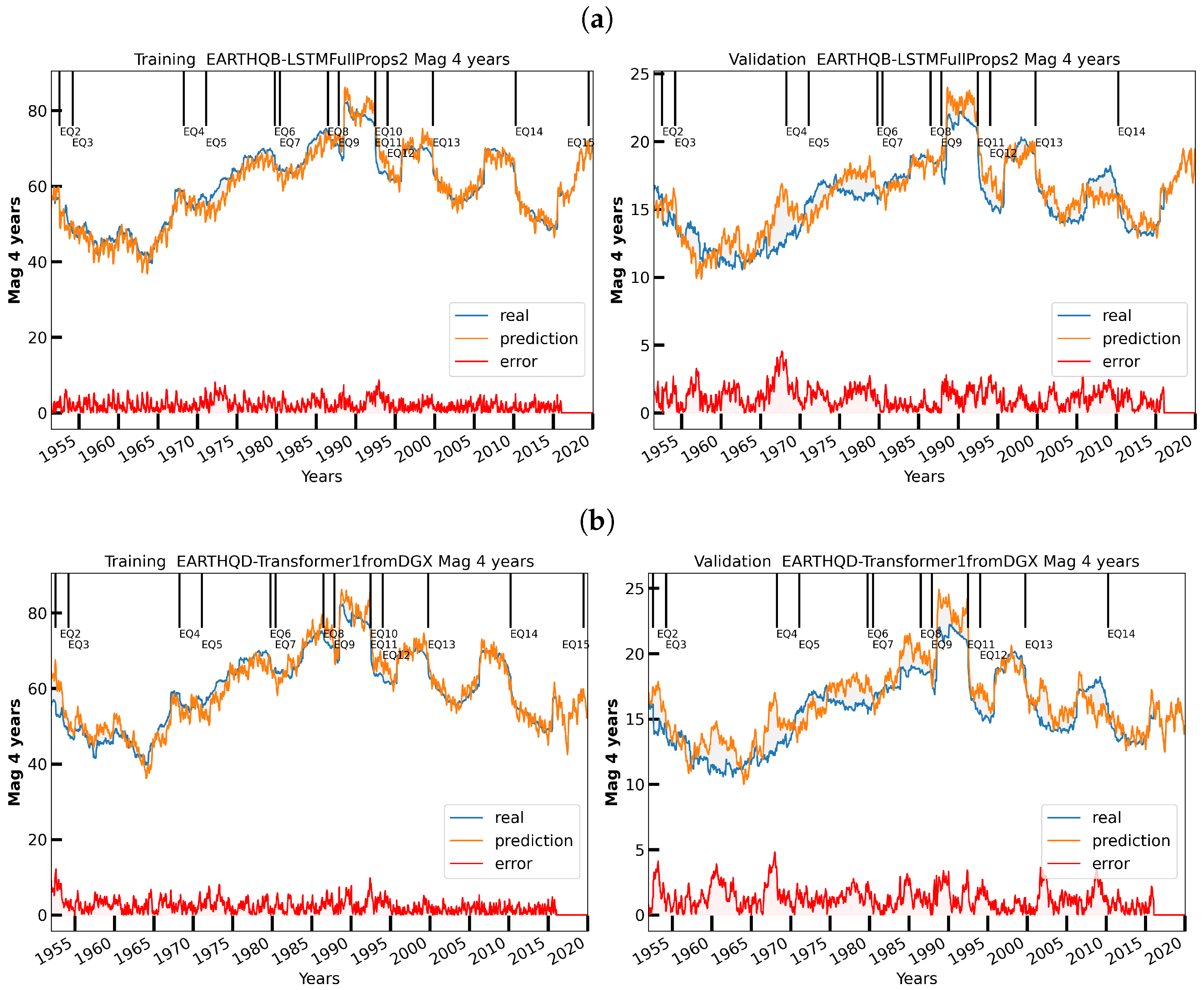
3.4. Visualizing the Data and Their Models

The scientific objective is to improve the quality of earthquake nowcasting and we explore deep learning in a region of Southern California, similar to that used in previous work [26,30]. This is quantified in a few metrics—the Nash Sutcliffe efficiency (NSE) [52] and in the visualization of predicted versus observed earthquake activity. NSE is a measure of a difference between the variation in the data over time with the discrepancy between observation and prediction so that predicting the observation to be the mean gives a default NSE of 0. The NSE is given in Equation (5) where quantity Q m t is model prediction at time t for quantity Q; Q o t is the observed value of Q at time t and Q o ¯ is the mean value of Q o t over time
N S E = 1 t = 1 t = T ( Q m t Q o t ) 2 t = 1 t = T ( Q o t Q o ¯ ) 2 .
We present results in the form of the normalized NSE [53], N N S E = 1 / ( 2 N S E ) , which runs between 0 (bad) and 1 (perfection) with NNSE = 0.5 corresponding to baseline prediction that the activity is equal to its time-averaged mean. This approach is common for the evaluation of time series models in other Earth science fields [54,55]. We supplement these overall averages with time-dependent plots of earthquake activity illustrated in Section 6.

4. Formulation of Deep Learning for Time Series

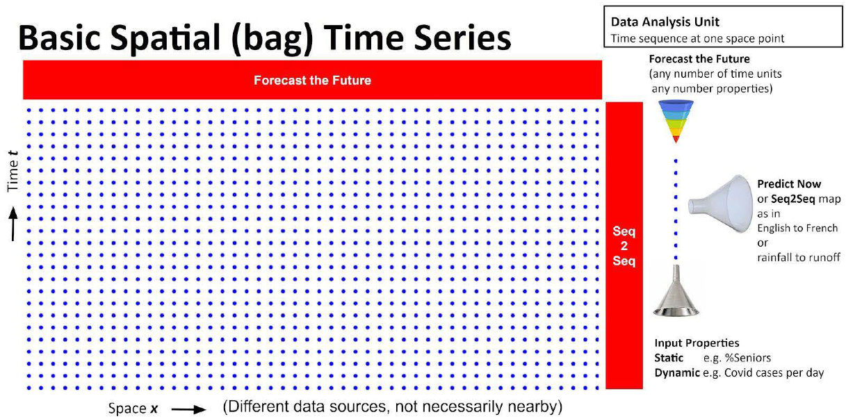
4.1. Spatial Bag Problem

We introduced the concept of a spatial bag for time series earlier and illustrate this in Figure 8, where we have a set of time series where the spatial distances (e.g., locality) between points are not important; rather they are differentiated by values of properties which can either be static (such as percentages of the population with high blood pressure for medical examples or minimum annual temperature for hydrology catchment studies) or dynamic (such as a local social distancing measure). In other papers, we will discuss problems that combine the features of spatial bags and distance locality where convolutional networks (especially convLSTM) are clearly useful. We tried convLSTM for the earthquake case but did not find it as effective as the methods reported here.

4.2. Deep Learning Implementations

Four distinct deep learning implementations will be considered:
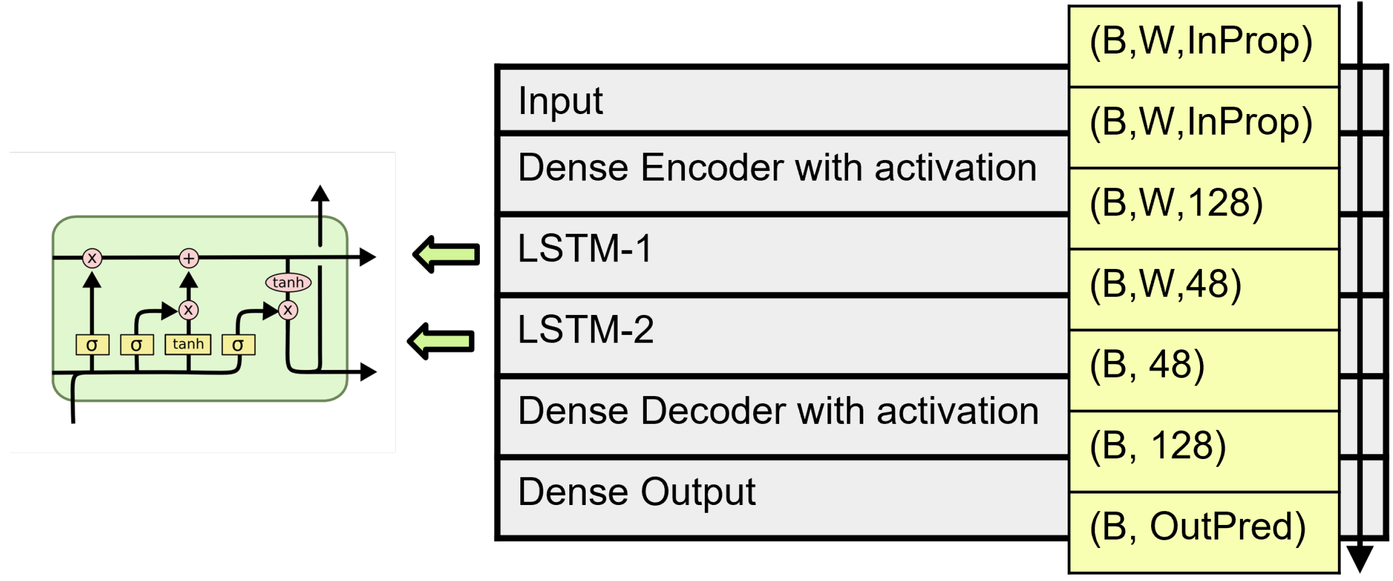
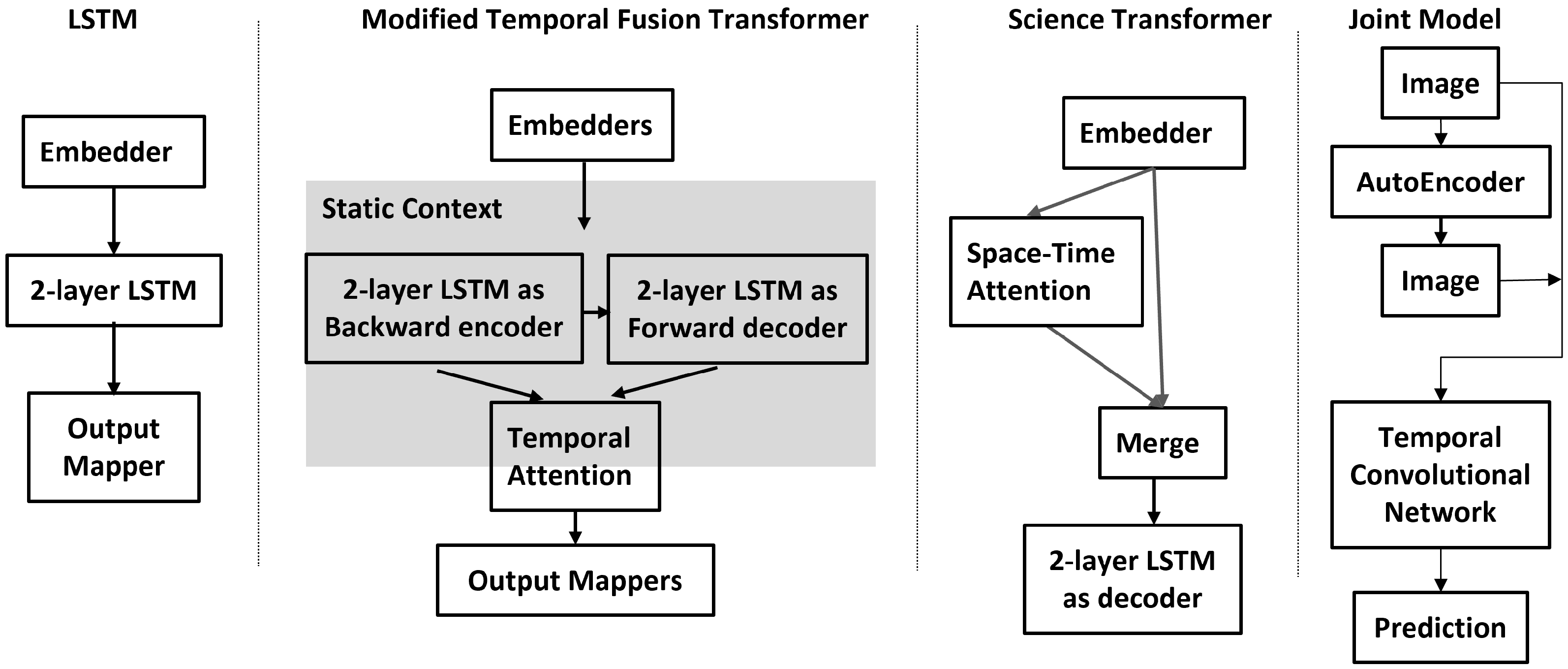
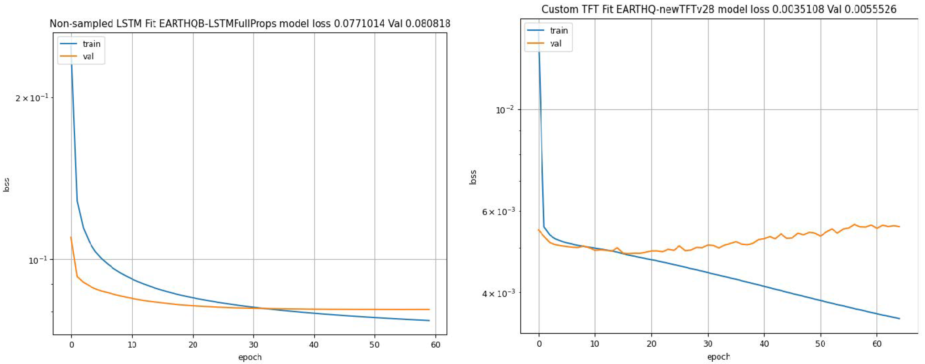
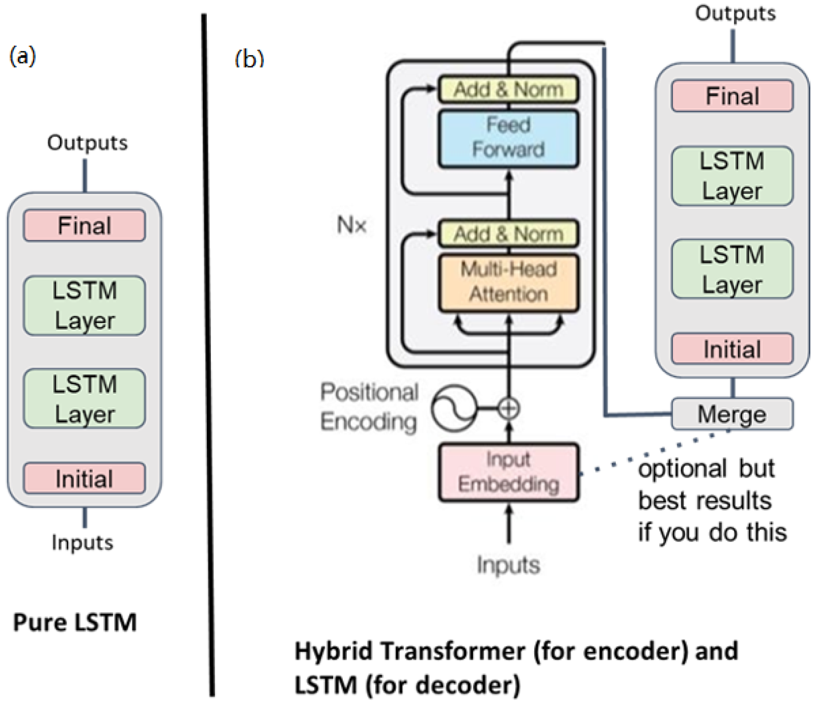
  • LSTM. Pure recurrent neural network—two-layer LSTM [56].
  • TFT. A version of the Google Temporal Fusion Transformer (TFT) [57,58] that uses two distinct LSTMs—one each for encoder and decoder with a temporal (attention-based) transformer.
  • Science Transformer. A hybrid model that was built at the University of Virginia with a space–time transformer for the decoder and a two-layer LSTM for the encoder.
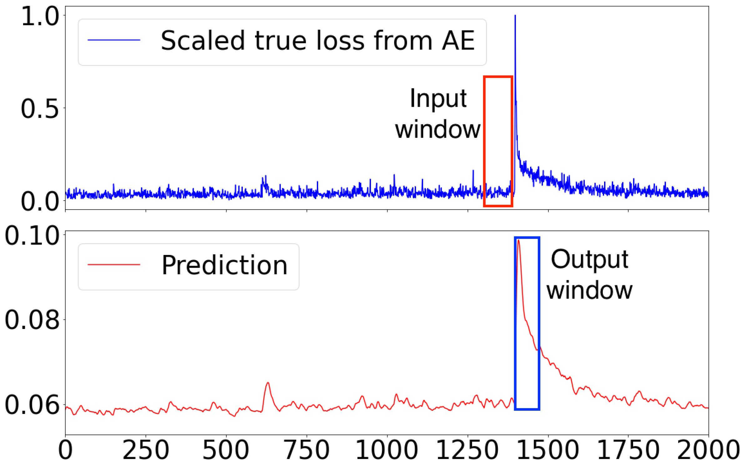
  • AE-TCN Joint Model. This is an architecture that combines two models. One is an autoencoder (AE) that encodes and decodes the image-like input and output. The other is a temporal convolutional network (TCN) which takes the differences from the input and output of the autoencoder and predicts the one-step future loss which is used to nowcast immediate earthquakes in refenerces [59,60].
All of these are programmed using the standard Tensorflow 2 class model. This required some adjustment for TFT for which the software is presented in Tensorflow 1 compatibility mode running under Tensorflow 2. NVIDIA has a modern version of the TFT with PyTorch [61]. We modified the TFT in a few ways to allow multiple targets and multilayer LSTMs. We also use mean square error (MSE) and not quantiles (mean absolute error) as the loss function. This loss is used identically in all 3 models. MSE appears more appropriate than MAE in this problem as it emphasizes the interesting large earthquake region; MAE weights small earthquakes more than MSE.

4.3. The Deep Learning Models in Detail

Deep learning models are typically constructed as a set of connected layers that calculate forward and back-propagation supported by the well-known PyTorch and Tensorflow frameworks. Each layer has parameters one can change, and the user can also vary the order and nature of layers. We have three implementations with rather different structures and sizes, which are summarized in Table 3. The smallest model is the LSTM with 6 layers shown in Figure 9 and 66,594 trainable parameters. Layers used include basic dense, dropout, activation, softmax, add, multiply as well as complex layers such as LSTM. The broad classes we use are a dense embedding layer for initial processing and a projection layer for final processing, transformers to identify patterns, and LSTM recurrent networks for time series processing. In other work, we have used autoencoders and temporal convolutional networks to identify earthquakes as extreme events [59,60]. We illustrate the simplest network in Figure 9 where gray represents layers and yellow-green data arrays with dimensions. The high-level architectures are compared in Figure 10 while the detailed TFT architecture is well described in references [57] and the other two models can be found in references [62,63].
Figure 11 gives typical plots of convergence of two of the models as a function of epoch. The models have different objective functions so absolute values cannot be compared. One can use results at any epoch trading off the training loss (which continues to decrease) with further epochs versus the validation loss which tends to stabilize.
The temporal fusion transformer has two important differences from the other two models. Firstly, it uses static variables to provide context (initial values) for several of the time-dependent steps. Secondly, it uses separate input embedders and output mappers for each variable whereas the other two methods use shared embedders and mappers. In future work, these TFT strategies should be considered in the other methods.

4.4. The Deep Learning Inputs and Outputs

Deep learning involves somewhat different inputs and outputs (predictions or targets) to more traditional approaches. Following [57], we identify three major classes of features which are functions of time (time series) for each member of the spatial bag (i.e., each pixel in Figure 6) or static characteristics of the bag member. These classes are Known Inputs, Observed Inputs, and Targets. We describe these in general and then specify how they were chosen for each model.
Observed Inputs are the basic measured quantities such as magnitude and depth of earthquakes. In the COVID-19 example illustrated in Figure 12, they are counts of daily infections and fatalities but also time-dependent auxiliary variables such as vaccination rate, measures of social distancing, hospitalization rates, etc. In the earthquake case, bin multiplicity counts are auxiliary variables. More formally, we divide observed inputs into “(a priori) unknown inputs” and targets as one typically has variables that are both observed inputs at times up to the current time and these need to be predicted and so fall in the target category as well.
Known Inputs are an interesting concept that includes both static features and time series (known time-dependent features). These are parameters that are known in both the past and future whereas observed inputs are only known in the past and need to be nowcast into the future. In the COVID-19 and earthquake examples, the only measured known inputs are the static features. In commercial applications, daily signatures of holidays or weekends are interesting inputs. Note these are categorical variables and generally all parameters can be categorical or come from a numerical scale. The latter tend to dominate scientific time series. In our analysis, we made extensive use of Mathematical Expansions which are functions of time in terms of which it appears natural to express the time dependence. In general, this is the place where simple models or theoretical intuition can be fed in but there is to date not much experience in exploiting this. As well as feeding in theoretical intuition in “known inputs” one can also feed in sophisticated functions of the observed data—such of those in our earlier work—as “observed inputs” allowing the deep learning to identify precursor patterns of future earthquakes.
Figure 12 shows the modified TFT applied to describe daily COVID-19 data up to 29 November 2021 (extended from references [56]). The weekly mathematical known input helps the model obtain a good description. The annual periodic variation was used to our advantage for describing hydrology data in ref. [63]. We also used Legendre polynomials as known inputs Pl(cosFull) where cosFull(t) varies from −1 to +1 over the full time range of the problem. The results here use the Legendre polynomials from l = 0 to 4. Note cosperiod(t), sinperiod(t), Pl(cosFull(t)) lie between −1 and +1 and fit the deep learning framework constraints quite well as they do not create poor ratios of mean/max of sizes. These are known inputs as they can be calculated for any time value—past or future.
Targets have already been introduced as these are the functions of time that we are trying to predict. They often include all or a subset of the observed inputs as for training they need to be known for times previous to when the nowcasting was made. However, just as we had unknown inputs that were time series which were not predicted, we also sometimes used Synthetic Targets that were predicted but not part of the input set. These need to be known for “all times” so they can be used in training.
However, inputs are best if they have no missing data, and this condition is not required for targets. These can be missing as we are using an additive loss function (MSE or MAE) and missing targets are just dropped from the sum in the loss function. We use this for predicting many years in the future which are dropped from training at times when the future measurements are not available. For example, if targets predict T forward time units into the future, we choose the maximum training time so the targets with the smallest forward time unit are known but not the others. In the simplest models, targets are the values of the observables at the final time. However, we also use synthetic futures when observables are m b i n ( F : Δ t , t ) integrals over time periods Δ t up to 4 years. Note that as we insist that inputs are all known, we only use backward input measurements for up to one year so we can start sequences one year after the data are first available. The final time value used is two weeks before the last date that data are available.
The choice of inputs and outputs is a fascinating area, and there is not much experience (community wisdom) on how best to do this. Deep learning networks employ far more learnable parameters (weights) than more traditional models, and this allows one to be rather profligate in the number of inputs and outputs. Note that modified steepest descent optimization methods used in deep learning optimization are very robust and allow everything to be large! There is some feeling that univariate (one output) problems are preferred, but we did not find this and used up to 24 output variables. The original TFT was restricted to univariate problems, but our multivariate extension was straightforward and appeared to perform well.
We now summarize in Table 4 and Table 5, the choices for the three networks discussed in this paper. Note that, for the LSTM and science transformer static, variables are implemented as known input time series with values independent of time. For the TFT, static variables are cleverly used to provide initial context for appropriate layer processing the true time series. Let us spell out the predicted values (targets) in Table 4 for the LSTM and science transformer. These are forward magnitudes m b i n for ten time intervals from 2 weeks up to 4 years in length. In addition, the network is asked to predict its inputs plus an integer labeling its spatial location. As stressed, at other times in this paper, our ideas are just a first look, and further research may suggest a different choice. Deep learning networks are very flexible and tolerant of idiosyncratic ideas.
The deep learning models are perhaps the important glamorous parts of the analysis but substantial data engineering is needed to preprocess the input data and visualize the results. This activity is described in ref. [19] and can be viewed in the online Jupyter notebooks.

5. Transformer and Attention Technologies

5.1. Using Transformers for Spatial Bags

The deep learning methods use approaches that were largely originally developed for natural language processing. Recurrent neural networks (RNNs) explicitly focus on sequences and pass them through a common network with subtle features. RNNs are designed to gather a history which allows the time dependence to be remembered. Attention-based methods [66] are more modern and perhaps somewhat easier to understand as attention is a simple idea.
NLP is basically a classification problem (look up tokens in a context-sensitive dictionary) whereas science tends to be numerical and so it is not immediately obvious how to use attention in technical time series and we describe one possible approach in this paper. There have been a few studies of transformer architectures for numerical time series such as references [67,68,69,70,71,72,73] but there is not a large literature.
Attention [4] means that one “learns” structure from other related data and looks for patterns using a simple “dot-product” mechanism, discussed later, matching the structure of different sequences; there are other approaches to match patterns which are a good topic for future work.
Here, we use for the science transformer mode a simple attention mechanism in an initial decoder but use a recurrent net LSTM for the encoder as shown in Figure 13. Such mixtures have been investigated and compared [74,75]. We compare the two architectures shown in Figure 13a,b.

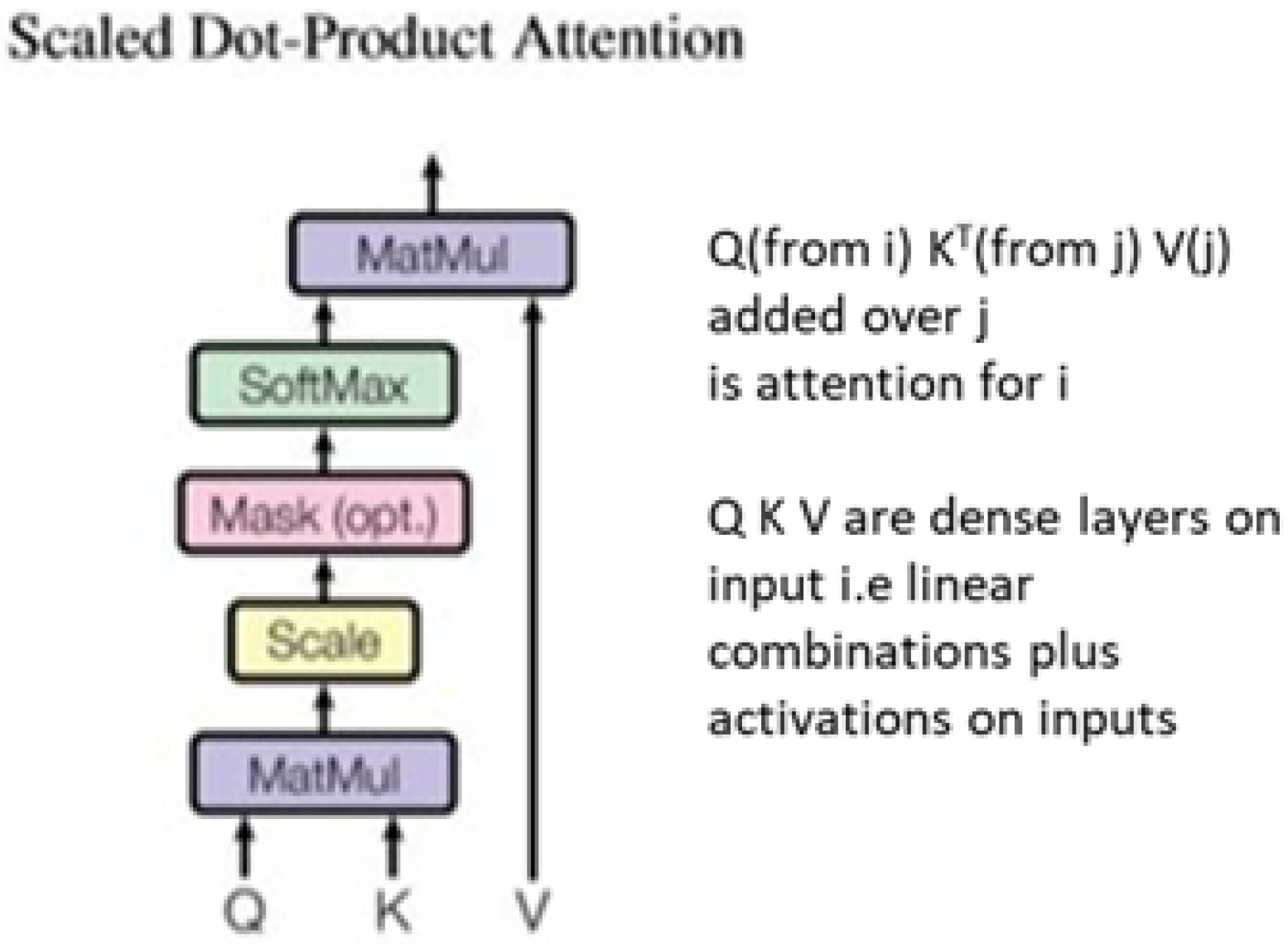
5.2. Scaled Dot-Product Attention and the Vectors Q K V

The basic sequence item for the LSTM and transformer models is the same, a space point with a time sequence with each time in the sequence having a set of static and dynamic values. In an LSTM, the sequence is “hidden” and one has to unroll the recurrent network to see it. However, in the transformer, the different time values in a sequence are treated directly and so each item contains W terms (W is the size of the time sequence). Each term is embedded in an input layer and then mapped by 3 different layers into vectors Q (query), K (key), V (value).
As shown in Figure 14, one matches terms i and j by calculating Q ( i ) K T ( j ) and ranking with a softmax step. This multiplies the characteristic vector V(j) of this pattern and the total attention A(i) for item i is calculated as a weighted sum over the values V(j). There are several different attention “heads” (networks generating Q, K, V) in each step and the whole process is repeated in multiple encoder layers. The result of the encoder step is considered separately for each item (each time in a time sequence at a given location) and the embedded input of this layer is combined with the attention as input to the LSTM decode step.

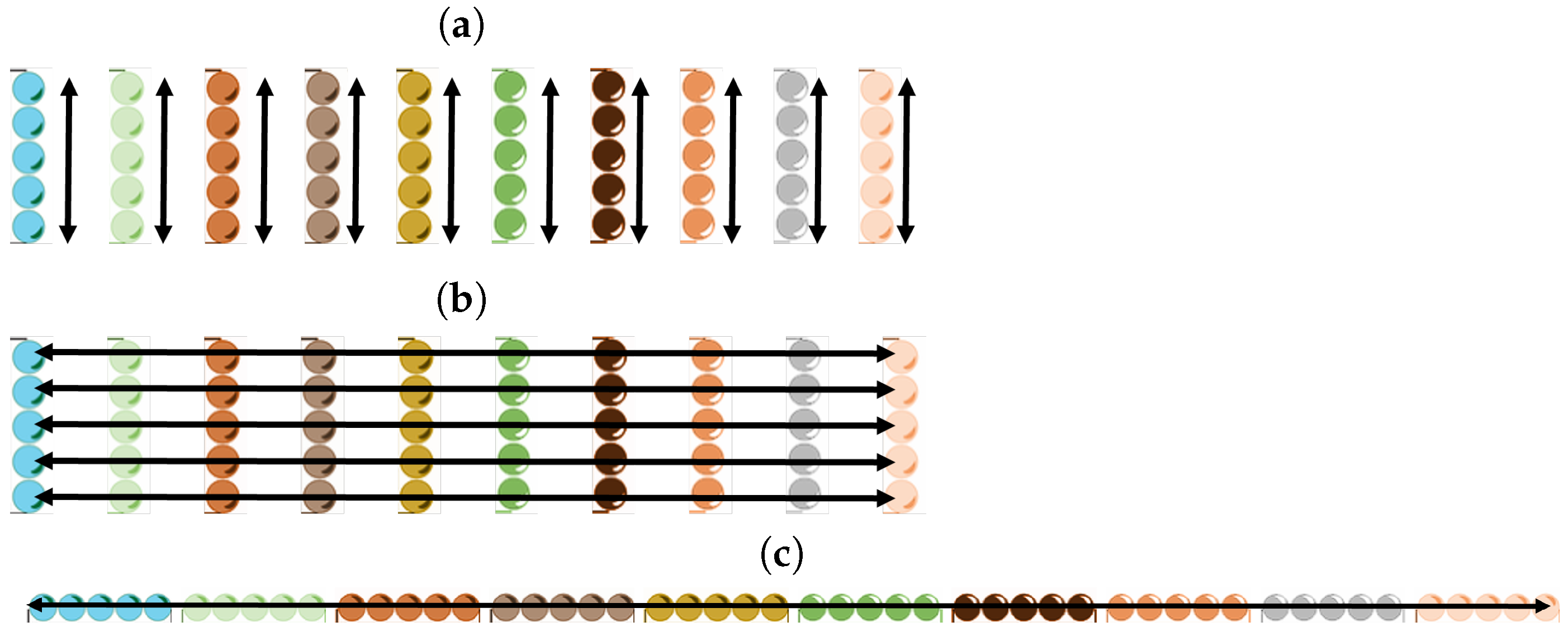
5.3. Choosing the Group of Items over Which Attention Is Calculated

In natural language processing, one looks for patterns among neighboring sentences, but for science time series, one can have larger regions as spatial bags with no locality. This leads to many choices as to the space over which attention is calculated as one cannot realistically consider all items simultaneously.
Suppose we have N l o c locations, each with N s e q sequences of length W. Then, the space to be searched has size N l o c * N s e q * W which is too large. In the COVID-19 example of Figure 12 [56], N l o c = 500 , N s e q ∼700, and W takes values up to 13 (the window size is naturally smaller in this case). In the hydrology example in ref. [63], N l o c = 671 , N s e q ∼7000, and W is up to 270. The next subsection describes the 3 search strategies we have looked at and are depicted in Figure 15. There is:
  • Temporal search: Points in sequence for fixed location.
  • Spatial search: Locations for a fixed position in the sequence.
  • Full search: Complete location–sequence space.
One will need to sample items randomly as only a small fraction of space is looked at in one attention step whatever method is used. Note that in all cases we used a batch size of 1 as the attention space was effectively the batch. Actually, in the LSTM stage, the different locations in the attention space were considered separately and the attention search space became the batch. In the work reported here, the attention space (and batch size) was set to N l o c but this is not required and would not work in some cases with large values of N l o c .
Even in the examples considered here, the search space can become so large that one needs to address memory size issues. Note that the encoding step of the transformer is many matrix multiplications and has excellent GPU performance, and, typically, the LSTM decoder would be a significant part of the compute time and so the addition of attention is not a major performance hurdle although it does require a large GPU memory. The TFT only uses temporal attention separately for each space point and so only the science transformer needs major (80 GB of A100) GPU memory.
An epoch contains N l o c * N s e q sequences, each of length W and consisting of static and dynamic variables characteristic of location. For an LSTM, one would have a batch that consists of NB N l o c sequences. The number of batches in an epoch is approximately N s e q . For a transformer, the batch is currently unwrapped as discussed above and used as the attention space. Memory usage or compute issues could require a different strategy separately considering batch and attention space.
Note that the attention space choice implies different initial shuffling to form batches and also different prediction stage approaches. For spatial and temporal searches, one can keep all locations at a particular time value together in both forming batches and in calculating predictions. For the full search, the complete set of N l o c * N s e q sequences must be shuffled. In practice, we combined the space–time and pure time searches and accumulated the results of these two attention searches.

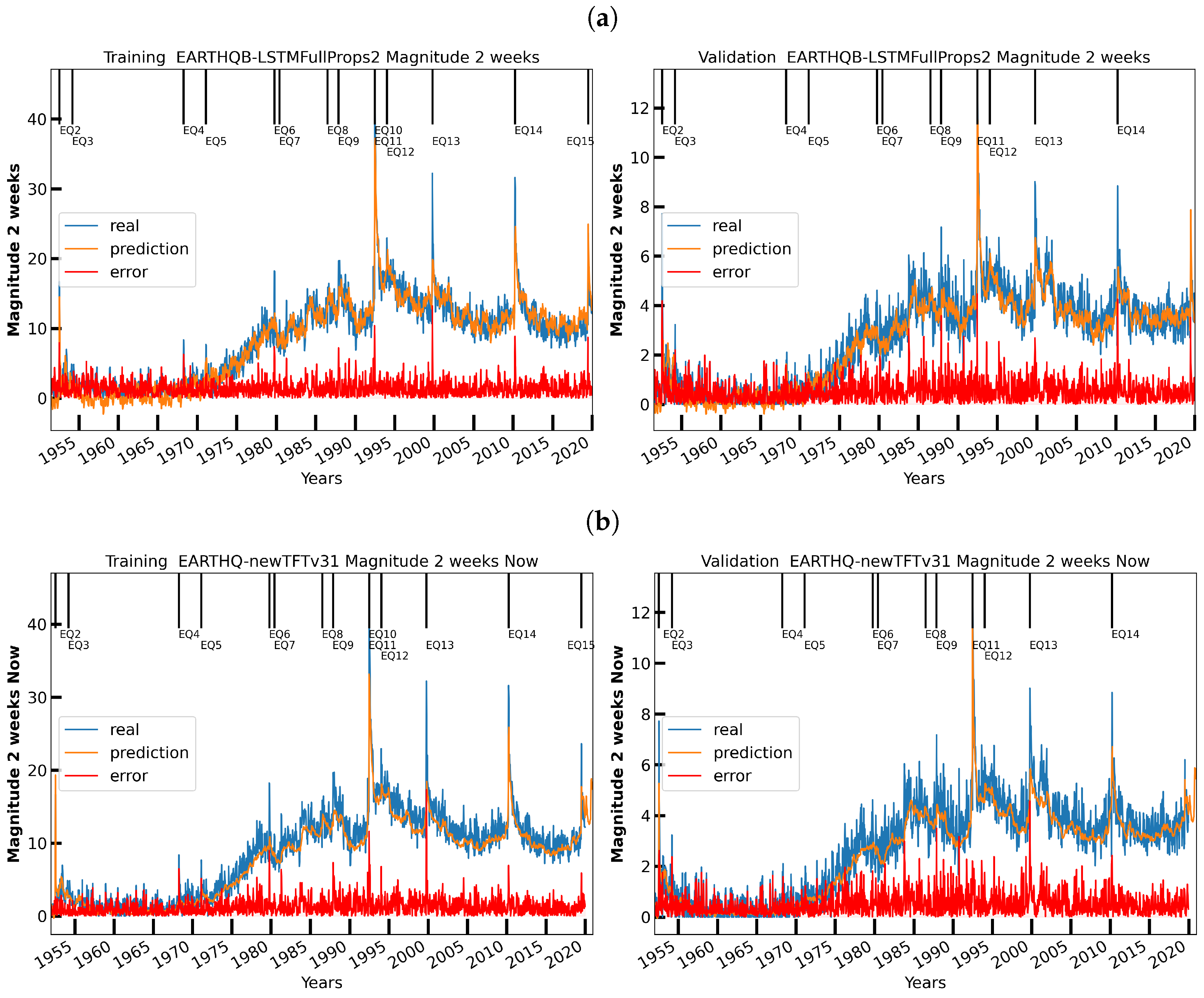
6. Initial Earthquake Nowcasting Results

6.1. Initial Results

These models give very detailed predictions over time and space and we can only illustrate them in this paper. We give a global summary with the Nash Sutcliffe efficiency and a sample of time-dependent results in figures of earthquake activity m b i n ( F : Δ t , t ) .
The NSE is given in Equation (5) where we use the normalized NSE, N N S E = 1 / ( 2 N S E ) , which runs between 0 (bad) and 1 (perfection). Table 6 gives the results for m b i n summed over all 400/100 locations. Note that all time interval bins use the forward m b i n described in Section 3 and Equation (1). Figure 16, Figure 17, Figure 18 and Figure 19 show the nowcasts for training and validation sets for a selection of four of ten prediction time intervals given in Table 4: two weeks, one year, two years, and four years. Each of these plots records the time of prominent earthquakes as a vertical dotted line. The data recorded are summed over all 400 training locations (on the left) and 100 validation locations (on the right). NNSE is not commonly used in the earthquake field and we should look at it in more detail in a range of other datasets/problem areas to understand any weaknesses or biases it might have.
The time period listed corresponds to the forward prediction of that length. The TFT only uses backward prediction but performs this for time steps reaching 26 weeks into the future, so the backward one-year value at t + 26 fortnights is the forward prediction at time t. It is not clear if the detailed 2-week predictions of TFT into the future (not given in other models) are valuable in this problem. We noted before that one cannot use these predictions to calculate cumulative observables as energy averaging and finding mean are not commutative. The current TFT implementation was not set up to nowcast all the time intervals covered by the other models and so this model is absent in some cells of Table 6 and in the later figures for 2-year and 4-year nowcasts. This is not intrinsic to the TFT model, and we will address this in future work, which can use larger memory machines to train networks that predict four years and not one year in the future as in our current TFT implementation. The TFT needs more memory to extrapolate further into the future as it predicts each time interval with a two-week interval in the four-year span, which needs significant memory. The other models have a different approach of viewing the multi time-interval predictions as associated with the initial time, and this leads to a memory use proportional to the number of time intervals predicted (10 here) compared to the number of 2-week time intervals extrapolated (108 for four years) for the TFT.
Turning to the results in Table 6, we find all the models giving results much larger than NNSE = 0.5, corresponding to a simple model that predicts all values to be time-averaged mean. The TFT has significantly better training results than the other two, and this is not surprising as Table 3 shows it has significantly more parameters than the other two models. As noted for Figure 11, one can trade off training and validation by choosing the epoch with which to generate the model. The TFT and science transformer would improve the description of the validation dataset and worsen that of the training dataset by defining the model with a lower epoch count. With the presented choice and the eight time intervals in Table 6, the TFT is best for two, and the LSTM and science transformer best for three each. In training, the TFT is best in the four time intervals predicted, and comparing the other models, the science transformer is best in five and the LSTM three. The superiority of the TFT in training is most pronounced for the smaller time intervals.
Looking at Figure 16, Figure 17, Figure 18 and Figure 19, we depict the observed data ( m b i n energy averaged in each location and summed over locations) in blue, the prediction in orange, and the difference in red. For both training and validation, all three models produce quite good descriptions of the observations with the largest discrepancies associated with the details of the large earthquakes. Note that a single large earthquake event produces a signal m b i n in one time interval in the two-week data but, in the four-year data, one event affects 104 time bins. Of course, preshocks and aftershocks broaden the large earthquake signal over multiple two-week bins.
The low probability of large earthquakes and their sporadic occurrence suggest that the larger time interval predictions, e.g., Figure 19, are especially valuable for nowcasts of the long-term hazard, and in future work, we could look at longer time intervals than four years. In Section 6.2, we address the different problems of anomaly nowcasting—near-term nowcasts of large quakes.
Table 7 summarizes some aspects of the Figure 16, Figure 17, Figure 18 and Figure 19. The table gives the mean square error for each figure separated for the first half (1950–1984) and second half (1985–2019) and it is presented separately for training and validation samples. Strikingly, for the 2-week data, the first half is predicted much better than the second half and all three models give very similar MSE values. The three longer time periods have better predictions for the second half compared to the first. Further, the models are rather different from each other in the quality of results. One might expect prediction quality to improve at later times as one only uses prior data in nowcasting the future and there are certainly more priors for the second half than the first. This table reinforces the slightly surprising conclusion that the smallest and simplest LSTM model performs as well as the more sophisticated transformer architectures in many of the predictions. This needs further study.

6.2. Nowcasting Extreme Events with AE-TCN Joint Model

The AE-TCN joint model is built as described in previous research [59,60] and an overview architecture is shown earlier in Figure 10. This research is an empirical study for predicting extreme shocks as major events controlled by a preconfigured threshold value. Figure 20 illustrates a result from a test set covering around 2000 data points, where each data point is an image-like snapshot of Southern California with pixels representing shock energy. We calculate the loss of the autoencoder as the mean absolute error from the reconstruction to the input. In Figure 20, the top sub-figure is the min–max scaled loss using the test dataset. The bottom sub-figure is the model prediction using the test dataset. A high value in prediction indicates the corresponding event is large. In the joint modeling, an autoencoder is responsible for encoding and decoding image input and a temporal convolutional network takes the differences from the autoencoder and predicts high loss, which indicates large events one step ahead.

7. Discussion and Conclusions

Above, we have presented an initial analysis of the use of deep learning for nowcasting earthquakes. We believe the methods are promising and have broad applicability across Earth science which offers many examples of geospatial time series. We have identified a class—spatial bags—where different space points are linked by different values of static labels and not directly by the geometry, We see very complex networks with from 60,000 to 8 million trainable (unknown) parameters. We use the data to develop the model which then replaces the physics description with these hidden variables.
It is known that the gradient descent optimization can use a redundant parametrization but still converge to a reasonable description. The network will over-train with many parameters, but by comparing training and validation loss one can find a good description, as presented here. This paper is not a definitive study, as it probes somewhat uncharted territory. In particular, we have made several heuristic choices that need further investigation, or in the deep learning parlance, one could say there are many hyperparameters in this problem that need to be explored.
Areas to explore include the choice of time unit (2 weeks here), the many parameters defining the networks, the targets, and the basic variable from m b i n to Energy (E) and its powers. We can also look at derived quantities such as those developed in earlier papers [24,25,26]. The choice of known inputs and the use of Fourier series and Legendre expansions need critical analysis; wavelets are discussed in ref. [76]. We also should explore the choice of the validation and testing sets as stressed in Section 3.2. We should use a full cross-validation and consider separating training and validation by cuts in time as well by dividing in space, as in this paper.
We noted earlier that the TFT had several clever methods that could be used in the LSTM and science transformer examples. The TFT team has recently come up with some interesting new ideas to explore [77]. Further, for the transformer, should one use temporal patterns as in TFT and AE-TCN or the space–time choice made in the science transformer. In doing this, we are looking at different regions including Southern California, Northern California, Washington State, Hawaii, and Alaska; further, we are exploring regions outside the USA. In such a multiregion analysis, we will gain insight into which features of the model and its results are reliable as they are valid in different regions. We are looking at a single model describing all regions as well as region-specific models. We are also examining the cut magnitude > 3.29 of this paper and the time intervals used; the data for some regions do not record small earthquakes, suggesting that a global model should use different data selections. In Section 3.4, we noted that the use of the Nash Sutcliffe efficiency is not well established in this field, and we could gain insight by baselining it in other earthquake models and looking at other activity measures.
The number of areas for further investigation is large partly because the aspects of our approach, discussed in the previous paragraph, have significant innovations. The choice of data follows our earlier papers and recurrent neural networks and transformers have been used in time series analysis. However, all the networks have been modified for this problem and only the LSTM has been used in previous publications [56] but with different types of targets with just a single time period. The use of custom known inputs and multitime period targets in Section 4.4 is a new idea as far as we know.
We intend to build a benchmark set of time series datasets and reference implementations as playing the same role for time series that ImageNet, ILSVRC, and AlexNet played for images. The different implementations establish best practices and can be used in different applications as already identified [78] in finance, networking, security, monitoring of complex systems from Tokamaks [79] to operating systems, and environmental science. This work will be performed in the MLCommons Science Data working group [80]. We intend to combine the open datasets and clean reference implementations available in MLCommons [81] with documentation and tutorials, which will allow MLCommons benchmarks to encourage the broad community to study these examples and use the ideas in other applications as well as improving on our base reference implementations. Of course, the purpose of this paper is “scientific discovery” and, similarly, this will be the main metric of the MLCommons science benchmarks. Here, we differ from other MLCommons benchmarks which largely stress hardware performance; that will be secondary for the science benchmarks.

Author Contributions

Conceptualization, J.B.R., A.D., G.C.F.; methodology, All; software, G.C.F. and B.F.; validation, all; data curation, B.F.; writing—original draft preparation, G.C.F.; writing—review and editing, all; visualization, all; All authors have read and agreed to the published version of the manuscript.

Funding

The work of G.C.F. and B.F. is partially supported by the National Science Foundation (NSF) through awards CIF21 DIBBS 1443054, CINES 1835598, and Global Pervasive Computational Epidemiology 1918626. We are grateful to Cisco University Research Program Fund grant 2020-220491 for supporting this research. Research by J.B.R. has been supported by a grant from the US Department of Energy to the University of California, Davis, DoE grant number DE- SC0017324, and by a grant from the National Aeronautics and Space Administration to the University of California, Davis, number NNX17AI32G. Portions of the research by Andrea Donnellan were carried out at the Jet Propulsion Laboratory, California Institute of Technology, under a contract with the National Aeronautics and Space Administration.

Institutional Review Board Statement

Not applicable.

Informed Consent Statement

Not applicable.

Data Availability Statement

The software is cited in Table 3 and data is from ref. [38].

Acknowledgments

We thank Tony Hey, Jeyan Thiyagalingam, Lijiang Guo, Gregor von Laszewski, Niranda Perera, Javier Toledo, Saumyadipta Pyne, Judy Fox, Xinyuan Huang, Russell Hofmann, Keerat Singh, JCS Kadupitiya, and Vikram Jadhao for great discussions. Sercan Arik and the Google TFT team were very helpful. The inspiration of MLCommons has been essential to guiding our research.

Conflicts of Interest

The authors declare no conflict of interest.

References

  1. Rundle, J.; Fox, G. Computational Earthquake Science. Comput. Sci. Eng. 2012, 14, 7–9. [Google Scholar] [CrossRef]
  2. Fox, G. FFFFWNPF-EARTHQD-Transformer1fromDGX DGX Jupyter Notebook for Science Transformer Forecast. Originally run 7 December 2021 on NVIDIA DGX but rehosted on Google Colab 15 March 2022. Available online: https://colab.research.google.com/drive/18yQ1RomlpHkCjRVwP4x5oBsyJ7WDoWwT?usp=sharing (accessed on 15 March 2022).
  3. Hey, T.; Trefethen, A. The Fourth Paradigm 10 Years On. Inform. Spektrum 2020, 42, 441–447. [Google Scholar] [CrossRef] [Green Version]
  4. Vaswani, A.; Shazeer, N.; Parmar, N.; Uszkoreit, J.; Jones, L.; Gomez, A.N.; Kaiser, Ł.; Polosukhin, I. Attention is all you need. In Advances in Neural Information Processing Systems; Guyon, I., Luxburg, U.V., Bengio, S., Wallach, H., Fergus, R., Vishwanathan, S., Garnett, R., Eds.; Curran Associates, Inc.: Dutchess County, NY, USA, 2017; Volume 30, pp. 5998–6008. [Google Scholar]
  5. Laptev, N.; Yosinski, J.; Li, L.E.; Smyl, S. Time-Series Extreme Event Forecasting with Neural Networks at Uber. In International Conference on Machine Learning. 2017, Volume 34, pp. 1–5. Available online: http://www.cs.columbia.edu/~lierranli/publications/TSW2017_paper.pdf (accessed on 10 April 2022).
  6. Li, Y.; Yu, R.; Shahabi, C.; Liu, Y. Diffusion convolutional recurrent neural network: Data-driven traffic forecasting. In Proceedings of the ICLR 2018 Conference, Vancouver, BC, Canada, 30 April–3 May 2018. [Google Scholar]
  7. Geng, X.; Li, Y.; Wang, L.; Zhang, L.; Yang, Q.; Ye, J.; Liu, Y. Spatiotemporal multi-graph convolution network for ride-hailing demand forecasting. In Proceedings of the AAAI Conference on Artificial Intelligence, Honolulu, HI, USA, 27 January–1 February 2019; Volume 33, pp. 3656–3663. [Google Scholar]
  8. Djuric, N.; Radosavljevic, V.; Cui, H.; Nguyen, T.; Chou, F.C.; Lin, T.H.; Singh, N.; Schneider, J. Uncertainty-aware short-term motion prediction of traffic actors for autonomous driving. In Proceedings of the IEEE/CVF Winter Conference on Applications of Computer Vision, Snowmass, CO, USA, 1–5 March 2020; IEEE Xplore 2020. pp. 2095–2104. Available online: https://arxiv.org/pdf/1808.05819.pdf (accessed on 7 December 2021).
  9. Ye, J.; Zhao, J.; Ye, K.; Xu, C. How to Build a Graph-Based Deep Learning Architecture in Traffic Domain: A Survey. IEEE Trans. Intell. Transp. Syst. 2020, 1–21. [Google Scholar] [CrossRef]
  10. Shen, C.; Penn State University. D2 2020 AI4ESS Summer School: Recurrent Neural Networks and LSTMs. Available online: https://www.youtube.com/watch?v=vz11tUgoDZc (accessed on 1 July 2020).
  11. Kratzert, F. CAMELS Extended Maurer Forcing Data. Available online: https://www.hydroshare.org/resource/17c896843cf940339c3c3496d0c1c077/ (accessed on 14 July 2020).
  12. Kratzert, F. Catchment-Aware LSTMs for Regional Rainfall-Runoff Modeling GitHub. Available online: https://github.com/kratzert/ealstm_regional_modeling (accessed on 14 July 2020).
  13. Kratzert, F.; Klotz, D.; Shalev, G.; Klambauer, G.; Hochreiter, S.; Nearing, G. Towards learning universal, regional, and local hydrological behaviors via machine learning applied to large-sample datasets. Hydrol. Earth Syst. Sci. 2019, 23, 5089–5110. [Google Scholar] [CrossRef] [Green Version]
  14. Addor, N.; Newman, A.J.; Mizukami, N.; Clark, M.P. The CAMELS data set: Catchment attributes and meteorology for large-sample studies. Hydrol. Earth Syst. Sci. 2017, 21, 21. [Google Scholar] [CrossRef] [Green Version]
  15. Sit, M.A.; Demiray, B.Z.; Xiang, Z.; Ewing, G.; Sermet, Y.; Demir, I. A Comprehensive Review of Deep Learning Applications in Hydrology and Water Resources. 2020. Available online: https://arxiv.org/ftp/arxiv/papers/2007/2007.12269.pdf (accessed on 7 December 2021).
  16. Liu, Y. Artificial Intelligence for Smart Transportation Video. Available online: https://slideslive.com/38917699/artificial-intelligence-for-smart-transportation (accessed on 8 August 2019).
  17. Yao, H.; Wu, F.; Ke, J.; Tang, X.; Jia, Y.; Lu, S.; Gong, P.; Ye, J.; Li, Z. Deep multi-view spatial-temporal network for taxi demand prediction. In Proceedings of the Thirty-Second AAAI Conference on Artificial Intelligence, New Orleans, LA, USA, 2–7 February 2018; AAAI: Menlo Park, CA, USA, 2018. [Google Scholar]
  18. Wu, Y.; Tan, H. Short-term traffic flow forecasting with spatial-temporal correlation in a hybrid deep learning framework. arXiv 2016, arXiv:1612.01022. [Google Scholar]
  19. Fox, G.C. Deep Learning for Spatial Time Series. Available online: https://www.researchgate.net/publication/346012611_DRAFT_Deep_Learning_for_Spatial_Time_Series?channel=doi&linkId=5fb5c04a92851c933f3d4ef1&showFulltext=true (accessed on 17 November 2020).
  20. Fox, G.; Rundle, J.; Feng, B. Study of Earthquakes with Deep Learning. Frankfurt Institute for Advanced Study Seismology & Artificial Intelligence Kickoff Workshop (Virtual). 2021. Available online: https://docs.google.com/presentation/d/1nTM-poaFzrT_KBB1J7BlZdOMEIMTu-s48mcBA5DeP30/edit#slide=id.g7a25695c64_0_0 (accessed on 7 December 2021).
  21. Guan, H.; Mokadam, L.K.; Shen, X.; Lim, S.H.; Patton, R. FLEET: Flexible Efficient Ensemble Training for Heterogeneous Deep Neural Networks. In Proceedings of Machine Learning and Systems. 2020; pp. 247–261. Available online: https://proceedings.mlsys.org/paper/2020/hash/ed3d2c21991e3bef5e069713af9fa6ca-Abstract.html (accessed on 1 December 2021).
  22. Scholz, C.H. The Mechanics of Earthquakes and Faulting; Cambridge University Press: Cambridge, UK, 2019. [Google Scholar]
  23. Rundle, J.B.; Stein, S.; Donnellan, A.; Turcotte, D.L.; Klein, W.; Saylor, C. The complex dynamics of earthquake fault systems: New approaches to forecasting and nowcasting of earthquakes. Rep. Prog. Phys. 2021, 84, 076801. [Google Scholar] [CrossRef]
  24. Rundle, J.B.; Donnellan, A. Nowcasting earthquakes in southern California with machine learning: Bursts, swarms, and aftershocks may be related to levels of regional tectonic stress. Earth Space Sci. 2020, 7, e2020EA001097. [Google Scholar] [CrossRef]
  25. Rundle, J.B.; Donnellan, A. Nowcasting earthquakes in southern California with machine learning: Bursts, swarms and aftershocks may reveal the regional tectonic stress. Earth Space Sci. Open Arch. 2020. [Google Scholar] [CrossRef]
  26. Rundle, J.B.; Donnellan, A.; Fox, G.; Crutchfield, J.P. Nowcasting Earthquakes by Visualizing the Earthquake Cycle with Machine Learning: A Comparison of Two Methods. Surv. Geophys. 2021. [Google Scholar] [CrossRef]
  27. Rundle, J.B.; Turcotte, D.L.; Donnellan, A.; Grant Ludwig, L.; Luginbuhl, M.; Gong, G. Nowcasting earthquakes. Earth Space Sci. 2016, 3, 480–486. [Google Scholar] [CrossRef]
  28. Savage, J.C. Principal component analysis of geodetically measured deformation in Long Valley caldera, eastern California, 1983-1987. J. Geophys. Res. 1988, 93, 13297–13305. [Google Scholar] [CrossRef]
  29. Tiampo, K.F.; Rundle, J.B.; McGinnis, S.; Gross, S.J.; Klein, W. Eigenpatterns in southern California seismicity. J. Geophys. Res. 2002, 107, ESE 8-1–ESE 8-17. [Google Scholar] [CrossRef]
  30. Rundle, J.B.; Donnellan, A.; Fox, G.; Crutchfield, J.P.; Granat, R. Nowcasting Earthquakes: Imaging the Earthquake Cycle in California with Machine Learning. Earth Space Sci. 2021, 8, e2021EA001757. [Google Scholar] [CrossRef]
  31. Kane, M.J.; Price, N.; Scotch, M.; Rabinowitz, P. Comparison of ARIMA and Random Forest time series models for prediction of avian influenza H5N1 outbreaks. BMC Bioinform. 2014, 15, 276. [Google Scholar] [CrossRef]
  32. Hochreiter, S.; Schmidhuber, J. Long Short-Term Memory. Neural Comput. 1997, 9, 1735–1780. Available online: http://xxx.lanl.gov/abs/https://direct.mit.edu/neco/article-pdf/9/8/1735/813796/neco.1997.9.8.1735.pdf (accessed on 7 December 2021). [CrossRef]
  33. Romero, R.A.C. Generative Adversarial Network for Stock Market Price Prediction. Available online: http://cs230.stanford.edu/projects_fall_2019/reports/26259829.pdf (accessed on 9 December 2021).
  34. Brownlee, J. A Gentle Introduction to Generative Adversarial Networks (GANs). Available online: https://machinelearningmastery.com/what-are-generative-adversarial-networks-gans/ (accessed on 9 December 2021).
  35. Wikipedia. Generative Adversarial Network. Available online: https://en.wikipedia.org/wiki/Generative_adversarial_network (accessed on 9 December 2021).
  36. Quinlan, J.R. Induction of decision trees. Mach. Learn. 1986, 1, 81–106. [Google Scholar] [CrossRef] [Green Version]
  37. Wikipedia. ID3 Algorithm. Available online: https://en.wikipedia.org/wiki/ID3_algorithm (accessed on 7 December 2021).
  38. Earthquake Hazards Program of United States Geological Survey. USGS Search Earthquake Catalog Home Page. Available online: https://earthquake.usgs.gov/earthquakes/search/ (accessed on 1 December 2020).
  39. Fox, G. Earthquake Data Used in Study “Earthquake Forecasting with Deep Learning”. Available online: https://drive.google.com/drive/folders/1wz7K2R4gc78fXLNZMHcaSVfQvIpIhNPi?usp=sharing (accessed on 1 December 2020).
  40. Field, E.H. Overview of the Working Group for the Development of Regional Earthquake Likelihood Models (RELM). Seismol. Res. Lett. 2007, 78, 7–16. [Google Scholar] [CrossRef]
  41. Quaternary Fault and Fold Database of the United States. Available online: https://www.usgs.gov/programs/earthquake-hazards/faults (accessed on 7 December 2021).
  42. Hanks, T.C.; Kanamori, H. A moment magnitude scale. J. Geophys. Res. Solid Earth 1979, 84, 2348–2350. [Google Scholar] [CrossRef]
  43. Benioff, H. Global strain accumulation and release as revealed by great earthquakes. GSA Bull. 1951, 62, 331–338. [Google Scholar] [CrossRef]
  44. Rundle, J.B.; Klein, W.; Turcotte, D.L.; Malamud, B.D. Precursory Seismic Activation and Critical-point Phenomena. In Microscopic and Macroscopic Simulation: Towards Predictive Modelling of the Earthquake Process; Mora, P., Matsu’ura, M., Madariaga, R., Minster, J.B., Eds.; Birkhäuser Basel: Basel, Switzerland, 2001; pp. 2165–2182. [Google Scholar]
  45. Ben-Zion, Y.; Lyakhovsky, V. Accelerated Seismic Release and Related Aspects of Seismicity Patterns on Earthquake Faults. In Earthquake Processes: Physical Modelling, Numerical Simulation and Data Analysis Part II; Matsu’ura, M., Mora, P., Donnellan, A., Yin, X.C., Eds.; Birkhäuser Basel: Basel, Switzerland, 2002; pp. 2385–2412. [Google Scholar]
  46. Newman, W.I.; Turcotte, D.L.; Gabrielov, A.M. log-periodic behavior of a hierarchical failure model with applications to precursory seismic activation. Phys. Rev. E Stat. Phys. Plasmas Fluids Relat. Interdiscip. Top. 1995, 52, 4827–4835. [Google Scholar] [CrossRef] [PubMed]
  47. Kadupitiya, J.C.S.; Fox, G.C.; Jadhao, V. Simulating Molecular Dynamics with Large Timesteps using Recurrent Neural Networks. arXiv 2020, arXiv:2004.06493. [Google Scholar]
  48. CIG Computational Infrastructure for Geodynamics. Virtual Quake Model for Earthquakes (Originally Virtual California). Available online: https://geodynamics.org/resources/1614/download/vq-1.1.0.tar.gz (accessed on 13 February 2022).
  49. Richards-Dinger, K.; Dieterich, J.H. RSQSim Earthquake Simulator. Seismol. Res. Lett. 2012, 83, 983–990. [Google Scholar] [CrossRef]
  50. Gilchrist, J.J.; Jordan, T.H.; Milner, K.R. Probabilities of Earthquakes in the San Andreas Fault System: Estimations from RSQSim Simulations. 2018, p. S41D-0569. Available online: https://www.scec.org/publication/8237 (accessed on 7 December 2021).
  51. Meyer, H.; Reudenbach, C.; Wöllauer, S.; Nauss, T. Importance of spatial predictor variable selection in machine learning applications—Moving from data reproduction to spatial prediction. Ecol. Model. 2019, 411, 108815. [Google Scholar] [CrossRef] [Green Version]
  52. Nash, J.; Sutcliffe, J. River flow forecasting through conceptual models part I—A discussion of principles. J. Hydrol. 1970, 10, 282–290. [Google Scholar] [CrossRef]
  53. Nossent, J.; Bauwens, W. Application of a normalized Nash-Sutcliffe efficiency to improve the accuracy of the Sobol’sensitivity analysis of a hydrological model. In EGU General Assembly Conference Abstracts. 2012, p. 237. Available online: https://meetingorganizer.copernicus.org/EGU2012/EGU2012-237.pdf (accessed on 7 December 2021).
  54. Patil, S.; Stieglitz, M. Modelling daily streamflow at ungauged catchments: What information is necessary? Hydrol. Process. 2014, 28, 1159–1169. [Google Scholar] [CrossRef] [Green Version]
  55. Feng, D.; Fang, K.; Shen, C. Enhancing streamflow forecast and extracting insights using long-short term memory networks with data integration at continental scales. Water Resour. Res. 2019, 56, e2019WR026793. [Google Scholar] [CrossRef]
  56. Fox, G.C.; von Laszewski, G.; Wang, F.; Pyne, S. AICov: An Integrative Deep Learning Framework for COVID-19 Forecasting with Population Covariates. J. Data Sci. 2021, 19, 293–313. [Google Scholar] [CrossRef]
  57. Lim, B.; Arık, S.Ö.; Loeff, N.; Pfister, T. Temporal fusion transformers for interpretable multi-horizon time series forecasting. Int. J. Forecast. 2021, 37, 1748–1764. [Google Scholar] [CrossRef]
  58. Kafritsas, N. Temporal Fusion Transformer: Time Series Forecasting with Interpretability Google’s State-of-the-Art Transformer Has It All. Available online: https://towardsdatascience.com/temporal-fusion-transformer-googles-model-for-interpretable-time-series-forecasting-5aa17beb621 (accessed on 7 December 2021).
  59. Feng, B.; Fox, G.C. TSEQPREDICTOR: Spatiotemporal Extreme Earthquakes Forecasting for Southern California. arXiv 2020, arXiv:2012.14336. [Google Scholar]
  60. Feng, B.; Fox, G.C. Spatiotemporal Pattern Mining for Nowcasting Extreme Earthquakes in Southern California. In Proceedings of the 2021 IEEE 17th International Conference on eScience, Innsbruck, Austria, 20–23 September 2021; pp. 99–107. [Google Scholar]
  61. TFT For PyTorch. Available online: https://catalog.ngc.nvidia.com/orgs/nvidia/resources/tft_for_pytorch (accessed on 7 December 2021).
  62. Fox, G. Study of Earthquakes with Deep Learning (Earthquakes for Real); Lectures in Class on AI First Engineering. Available online: https://docs.google.com/presentation/d/1ykYnX0uvxPE-M-c-Tau8irU3IqYuvj8Ws8iUqd5RCxQ/edit?usp=sharing (accessed on 30 September 2021).
  63. Fox, G. Deep Learning Based Time Evolution. Available online: http://dsc.soic.indiana.edu/publications/Summary-DeepLearningBasedTimeEvolution.pdf (accessed on 8 June 2020).
  64. Fox, G. FFFFWNPF-EARTHQB-LSTMFullProps2 Google Colab for LSTM Forecast. Available online: https://colab.research.google.com/drive/16DjDXv8wjzNm7GABNMCGiE-Q0gFAlNHz?usp=sharing (accessed on 7 December 2021).
  65. Fox, G. FFFFWNPFEARTHQ-newTFTv29 Google Colab for TFT Forecast. Available online: https://colab.research.google.com/drive/12zEv08wvwRhQEwYWy641j9dLSDskxooG?usp=sharing (accessed on 7 December 2021).
  66. Galassi, A.; Lippi, M.; Torroni, P. Attention in Natural Language Processing. arXiv 2019, arXiv:1902.02181. [Google Scholar] [CrossRef] [PubMed]
  67. Kaji, D.A.; Zech, J.R.; Kim, J.S.; Cho, S.K.; Dangayach, N.S.; Costa, A.B.; Oermann, E.K. An attention based deep learning model of clinical events in the intensive care unit. PLoS ONE 2019, 14, e0211057. [Google Scholar] [CrossRef] [PubMed] [Green Version]
  68. Gangopadhyay, T.; Tan, S.Y.; Jiang, Z.; Meng, R.; Sarkar, S. Spatiotemporal Attention for Multivariate Time Series Prediction and Interpretation. In Proceedings of the 2021 IEEE International Conference on Acoustics, Speech and Signal Processing (ICASSP), Toronto, ON, Canada, 6–11 June 2021; pp. 3560–3564. [Google Scholar] [CrossRef]
  69. Xu, N.; Shen, Y.; Zhu, Y. Attention-Based Hierarchical Recurrent Neural Network for Phenotype Classification. In Advances in Knowledge Discovery and Data Mining; Springer International Publishing: Berlin/Heidelberg, Germany, 2019; pp. 465–476. [Google Scholar]
  70. Kodialam, R.S.; Boiarsky, R.; Sontag, D. Deep Contextual Clinical Prediction with Reverse Distillation. In Proceedings of the 35th AAAI Conference on Artificial Intelligence, Vancouver, BC, Canada, 2–9 February 2021; pp. 249–258. [Google Scholar]
  71. Gao, J.; Wang, X.; Wang, Y.; Yang, Z.; Gao, J.; Wang, J.; Tang, W.; Xie, X. CAMP: Co-Attention Memory Networks for Diagnosis Prediction in Healthcare. In Proceedings of the 2019 IEEE International Conference on Data Mining (ICDM), Beijing, China, 8–11 November 2019; pp. 1036–1041. [Google Scholar]
  72. Sen, R.; Yu, H.F.; Dhillon, I. Think Globally, Act Locally: A Deep Neural Network Approach to High-Dimensional Time Series Forecasting. Available online: https://assets.amazon.science/44/a7/9f453036411b93f79f1fe3e933ff/think-globally-act-locally-a-deep-neural-network-approach-to-high-dimensional-time-series-forecasting.pdf (accessed on 7 December 2021).
  73. Song, H.; Rajan, D.; Thiagarajan, J.J.; Spanias, A. Attend and diagnose: Clinical time series analysis using attention models. In Proceedings of the Thirty-Second AAAI Conference on Artificial Intelligence, New Orleans, LA, USA, 2–7 February 2018. [Google Scholar]
  74. Zeyer, A.; Bahar, P.; Irie, K.; Schlüter, R.; Ney, H. A Comparison of Transformer and LSTM Encoder Decoder Models for ASR. In Proceedings of the 2019 IEEE Automatic Speech Recognition and Understanding Workshop (ASRU), Sentosa, Singapore, 14–18 December 2019; pp. 8–15. [Google Scholar]
  75. Zeng, Z.; Pham, V.T.; Xu, H.; Khassanov, Y.; Chng, E.S.; Ni, C.; Ma, B. Leveraging Text Data Using Hybrid Transformer-LSTM Based End-to-End ASR in Transfer Learning. In Proceedings of the 12th International Symposium on Chinese Spoken Language Processing (ISCSLP), Piscataway Township, NJ, USA, 24–26 January 2021. [Google Scholar]
  76. Rhif, M.; Ben Abbes, A.; Farah, I.R.; Martínez, B.; Sang, Y. Wavelet Transform Application for/in Non-Stationary Time-Series Analysis: A Review. Appl. Sci. 2019, 9, 1345. [Google Scholar] [CrossRef] [Green Version]
  77. Arik, S.O.; Yoder, N.C.; Pfister, T. Self-Adaptive Forecasting for Improved Deep Learning on Non-Stationary Time-Series. arXiv 2022, arXiv:2202.02403. [Google Scholar]
  78. Huang, X.; Fox, G.C.; Serebryakov, S.; Mohan, A.; Morkisz, P.; Dutta, D. Benchmarking Deep Learning for Time Series: Challenges and Directions. In Proceedings of the 2019 IEEE International Conference on Big Data (Big Data), Los Angeles, CA, USA, 9–12 December 2019; pp. 5679–5682. [Google Scholar]
  79. Kates-Harbeck, J.; Svyatkovskiy, A.; Tang, W. Predicting disruptive instabilities in controlled fusion plasmas through deep learning. Nature 2019, 568, 526–531. [Google Scholar] [CrossRef]
  80. Fox, G.; Hey, T.; Thiyagalingam, J. Science Data Working Group of MLCommons. Available online: https://mlcommons.org/en/groups/research-science/ (accessed on 3 December 2020).
  81. MLCommons Homepage: Machine Learning Innovation to Benefit Everyone. Available online: https://mlcommons.org/en/ (accessed on 7 December 2021).
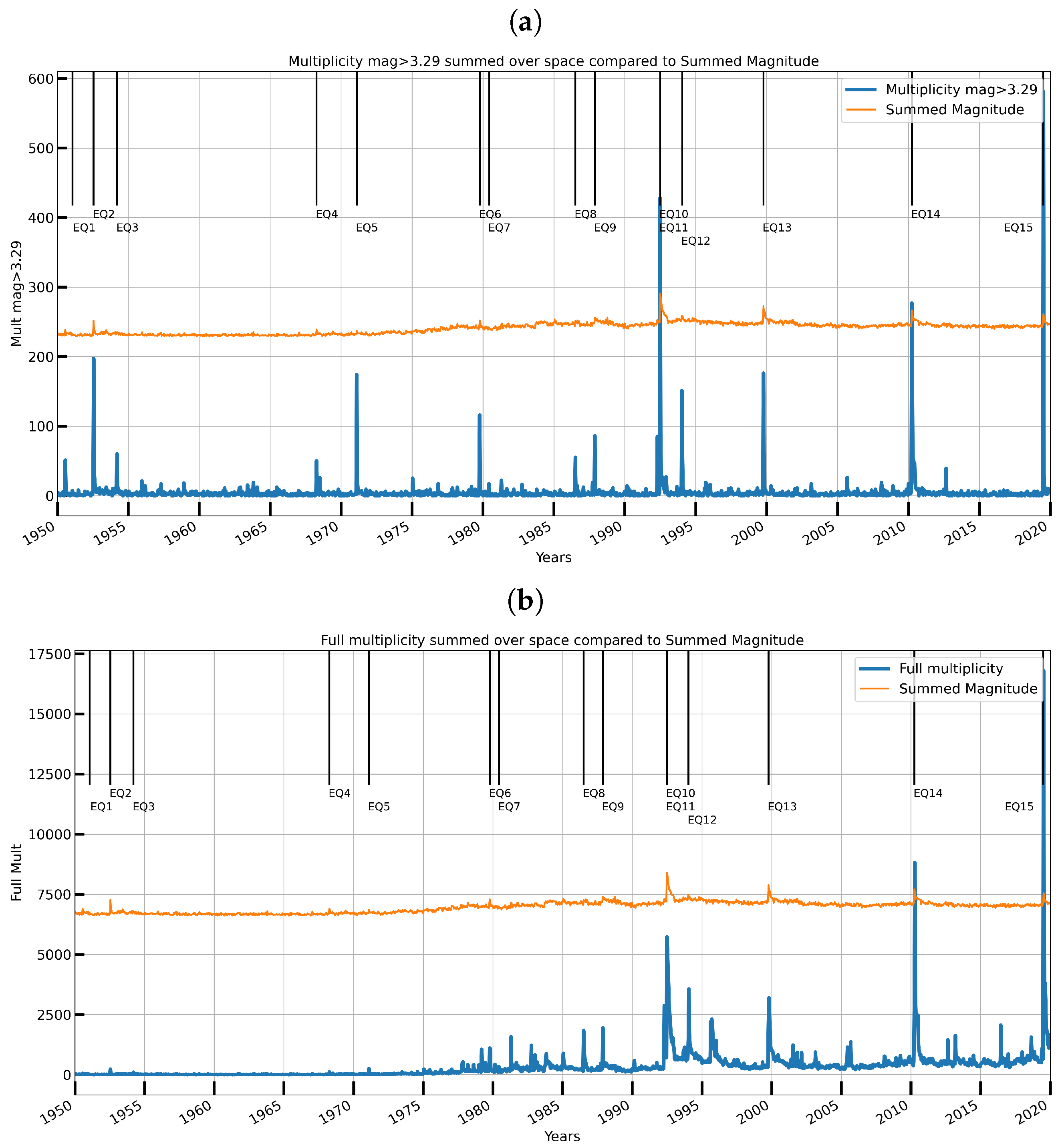
Figure 1. Comparison of traditional theory-driven analysis (left) with the data-driven ideas (right).
Geohazards 03 00011 g001
Figure 2. Example of a nowcast for M6 earthquakes near Los Angeles.
Geohazards 03 00011 g002
Figure 3. Earthquake burst nowcasting.
Geohazards 03 00011 g003
Figure 4. An example of a time series prediction using the RFC method.
Geohazards 03 00011 g004
Figure 5. Comparisons of time dependence of four different measures of earthquake activity with m b i n . The earthquakes marked are listed in Table 1. (a) Time dependence of Multiplicity > 3.29 events compared to m b i n of Equation (1). (b) Time dependence of Multiplicity of all events compared to m b i n of Equation (1). (c) Time dependence of E n e r g y 0.25 in fortnightly bins compared to m b i n of Equation (1). Note the suppressed zero in plot. (d) Time dependence of E n e r g y 0.25 in fortnightly bins compared to m b i n of Equation (1).
Geohazards 03 00011 g005aGeohazards 03 00011 g005b
Figure 6. The 500 spatial regions (pixels) used in the analysis are divided randomly into 400 red training and 100 green validation/testing pixels with the remaining 1900 regions in shades of gray.
Geohazards 03 00011 g006
Figure 7. Region studied showing earthquake activity (a,b); raw faults in (c); and grouped fault regions in (d). (a) Region studied as a standard map; the redder regions represent earthquakes of higher magnitude. (b) Region studied on a satellite map; the redder regions represent earthquakes of higher magnitude. (c) Fault lines [41] grouped together in (d). (d) Fault regions [41] after fault grouping together with a particular space-filling label for each of the 2400 pixels.
Geohazards 03 00011 g007
Figure 8. Illustration of a spatial bag with associated time sequences. t labels time and x location. The Seq2Seq and forecast modes are illustrated as well as the structure of input data and predictions.
Geohazards 03 00011 g008
Figure 9. LSTM deep learning network used in this analysis. The 2 LSTM layers are sophisticated compound networks illustrated on the left. B is batch size (400), W is window size (13); InProp is the number of input time series (27) and OutPred the number of predicted time series (24).
Geohazards 03 00011 g009
Figure 10. High-level architectures of four deep learning networks.
Geohazards 03 00011 g010
Figure 11. Epoch dependence of training and validation loss for LSTM (left) and TFT (right).
Geohazards 03 00011 g011
Figure 12. Modified TFT description of 500 most populous counties in the USA for COVID-19 daily infection and fatality data showing strong weekly periodic structure from early 2020 to November. Individual counties are scaled so all lie between 0 and 1 and the figure shows the sum of the square root of the number of recorded daily events in 2021.
Geohazards 03 00011 g012
Figure 13. (a) Pure LSTM and (b) science transformer models discussed in this paper. The former just uses a two-layer recurrent neural network while the latter has an attention-based encoder and an LSTM-based final decoder.
Geohazards 03 00011 g013
Figure 14. The Q, K, V layers of the attention mechanism.
Geohazards 03 00011 g014
Figure 15. Three search strategies discussed in this paper. N = N A is the number of items considered in attention search—each labeled with a location and starting time—and each has a window of length W. W = 5 in the diagram. N A = N B = N l o c here. (a) Temporal: At each location, look over time window O ( N W 2 ) . (b) Spatial: Look across items at fixed position in time window O ( N 2 W ) . (c) Full: Look over all space time windows in batch O ( N 2 W 2 ) .
Geohazards 03 00011 g015
Figure 16. Two-week m b i n ( F : Δ t , t ) results for Δ t = 2 weeks (training on left, validation on the right) are given for 3 methods. The earthquakes marked are listed in Table 1. (a) Two-week LSTM results for m b i n ( F : Δ t , t ) for Δ t = 2 weeks. (b) Two-week TFT results for m b i n ( F : Δ t , t ) for Δ t = 2 weeks. (c) Two-week science transformer results for m b i n ( F : Δ t , t ) for Δ t = 2 weeks.
Geohazards 03 00011 g016aGeohazards 03 00011 g016b
Figure 17. One-year m b i n ( F : Δ t , t ) results for Δ t = 52 weeks (training on left, validation on the right) are given for 3 methods. The earthquakes marked are listed in Table 1. (a) One-year LSTM results for m b i n ( F : Δ t , t ) for Δ t = 52 weeks. (b) One-year TFT results for m b i n ( F : Δ t , t ) for Δ t = 52 weeks. Note TFT results are formed using m b i n ( F : Δ t , t ) = m b i n ( B : Δ t , t + Δ t ) . (c) One-year science transformer results for m b i n ( F : Δ t , t ) for Δ t = 52 weeks.
Geohazards 03 00011 g017aGeohazards 03 00011 g017b
Figure 18. Two-year m b i n ( F : Δ t , t ) results for Δ t = 104 weeks (training on left, validation on the right) are given for 2 methods (TFT not available). The earthquakes marked are listed in Table 1. (a) Two-year LSTM results for m b i n ( F : Δ t , t ) for Δ t = 104 weeks. (b) Two-year science transformer results for m b i n ( F : Δ t , t ) for Δ t = 104 weeks.
Geohazards 03 00011 g018
Figure 19. Four-year m b i n ( F : Δ t , t ) results for Δ t = 208 weeks (training on left, validation on the right) are given for 2 methods (TFT not available). The earthquakes marked are listed in Table 1. (a) Four-year LSTM results for m b i n ( F : Δ t , t ) for Δ t = 208 weeks. (b) Four-year science transformer results for m b i n ( F : Δ t , t ) for Δ t = 208 weeks.
Geohazards 03 00011 g019
Figure 20. An empirical study with the autoencoder (AE)–temporal convolutional network (TCN) joint model.
Geohazards 03 00011 g020
Table 1. Fifteen earthquakes from the earthquake catalog data [38] shown in plots.
LabelDateMagnitudeLocation
EQ124 January 19516.014 km WNW of Tecolots, B.C., MX
EQ221 July 19527.56 km WNW of Grapevine, CA
EQ319 March 19546.412 km W of Salton City, CA
EQ49 April 19686.65 km NNE of Ocotillo Wells, CA
EQ59 February 19716.610 km SSW of Agua Dulce, CA
EQ615 October 19796.410 km E of Mexicali, B.C., MX
EQ79 June 19806.35 km SE of Alberto Oviedo Mota, B.C., MX
EQ89 July 19866.06 km SSW of Morongo Valley, CA
EQ924 November 19876.622 km W of Westmorland, CA
EQ1028 June 19927.3Landers, California Earthquake
EQ1128 June 19926.37 km SSE of Big Bear City, CA
EQ1217 January 19946.71 km NNW of Reseda, CA
EQ1316 October 19997.1Hector Mine, CA Earthquake
EQ144 April 20107.212 km SW of Delta, B.C., MX
EQ154 July 20196.4Ridgecrest Earthquake Sequence
Table 2. Ratios of mean to the maximum of potential observables.
Ratio Mean/Max for Observables m bin Full MultiplicityMultiplicity m > 3.29 E 0.25 E 0.5
Individual pixels0.110.00000460.0000220.00320.000016
Summed over space0.830.0120.00790.530.025
Table 3. Some features of the 3 models. The # layers are only for the highest level and nearly all of them are composite, so the full count is much higher.
Network# Layers# Trainable ParametersWindow SizeInternal Label and Online Link
LSTM666,59013EARTHQB-LSTMFullProps2 [64]
TFT738,005,33426EARTHQ-newTFTv29 [65]
Science Transformer142,339,32826FFFFWNPF-EARTHQD-Transformer1fromDGX [2]
Table 4. Input and output variables for the LSTM and science transformer.
Static Known Inputs (5)Four space-filling curve labels of fault grouping, linear label of pixel
Targets (24) m b i n ( F : Δ t , t ) for Δ t = 2, 4, 8, 14, 26, 52, 104, 208 weeks. Additionally, for skip 52 weeks and predict next 52 weeks; skip 104 weeks and predict next 104 weeks. With relative weight 0.25, all the Known Inputs and linear label of pixel
Dynamic Known Inputs (13) P l ( cos θ F u l l ) for l = 0 to 4
cos θ p e r i o d ( t ) , sin θ p e r i o d ( t ) for period = 8, 16, 32, 64
Dynamic Unknown Inputs (9)Energy-averaged Depth, Multiplicity, Multiplicity m > 3.29 events m b i n ( B : Δ t , t ) for Δ t = 2, 4, 8, 14, 26, 52 weeks
Table 5. Input and output variables for the modified temporal fusion transformer.
Static Known Inputs (5)Four space-filling curve labels of fault grouping, linear label of pixel
Targets (4) m b i n ( F : Δ t , t ) for Δ t = 2, 14, 26, 52 weeks. Calculated for t-52 to t for encoder and t to t + 52 weeks for decoder in 2 week intervals. One hundred and four predictions per sequence
Dynamic Known Inputs (13) P l ( cos θ F u l l ) for l = 0 to 4
cos θ p e r i o d ( t ) , sin θ p e r i o d ( t ) for period = 8, 16, 32, 64
Dynamic Unknown Inputs (9)Energy-averaged Depth, Multiplicity, Multiplicity m > 3.29 events m b i n ( B : Δ t , t ) for Δ t = 2, 4, 8, 14, 26, 52 weeks
Table 6. Summary of nowcasting results in terms of predicted Nash Sutcliffe efficiencies.
Normalized Nash Sutcliffe Efficiency (NNSE)
Time PeriodLSTM TrainTFT TrainScience Transformer TrainLSTM ValidationTFT ValidationScience Transformer Validation
2 weeks0.9030.9150.8930.8680.8750.856
4 weeks0.895 0.9160.867 0.884
8 weeks0.886 0.9130.866 0.881
14 weeks0.9240.9630.9190.8930.9050.881
26 weeks0.9460.9560.9540.8970.8920.896
52 weeks0.9190.9570.9550.8610.8710.876
104 weeks0.923 0.9370.853 0.83
208 weeks0.935 0.9210.811 0.77
Table 7. Mean square error over first and second 35-year periods of data averaged over location and two-week time interval.
Time PeriodMSELSTMTFTScience Transformer
First HalfSecond HalfFirst HalfSecond HalfFirst HalfSecond Half
Two weeksTraining0.00260.00350.00250.00350.00250.0035
Validation0.00290.00370.00290.00370.00290.0037
One yearTraining0.00960.00630.00700.00360.00830.0053
Validation0.0110.00730.0130.00850.0110.0074
Two yearsTraining0.0110.0069N/AN/A0.00950.0058
Validation0.0140.0086N/AN/A0.0160.012
Four yearsTraining0.0110.0079N/AN/A0.00950.0058
Validation0.0150.011N/AN/A0.0160.012
Publisher’s Note: MDPI stays neutral with regard to jurisdictional claims in published maps and institutional affiliations.

