Article

Correlation Dimension in Sumatra Island Based on Active Fault, Earthquake Data, and Estimated Horizontal Crustal Strain to Evaluate Seismic Hazard Functions (SHF)

1
Faculty of Mining and Petroleum Engineering, Bandung Institute of Technology, Bandung 40132, Indonesia
2
Faculty of Earth Sciences and Technology ITB, Bandung Institute of Technology, Bandung 40132, Indonesia
3
National Research and Innovation Agency (BRIN), Jakarta 10340, Indonesia
*
Author to whom correspondence should be addressed.
GeoHazards 2022, 3(2), 227-241; https://doi.org/10.3390/geohazards3020012
Submission received: 6 January 2022 / Revised: 14 April 2022 / Accepted: 19 April 2022 / Published: 22 April 2022
(This article belongs to the Topic Natural Hazards and Disaster Risks Reduction)

Abstract

:
This study intends to evaluate the possible correlation between the correlation dimension (DC) and the seismic moment rate for different late Quaternary active fault data, shallow crustal earthquakes, and GPS on the island of Sumatra Probabilistic Seismic Hazard Analysis (PSHA). The seismicity smoothing was applied to estimate the DC of active faults (DF) and earthquake data (DE) and then to correlate that with the b-value, which will be used to identify seismic hazard functions (SHF) along with the Sumatra Fault Zone (SFZ). The seismicity based on GPS data was calculated by the seismic moment rate that is estimated based on pre-seismic horizontal surface displacement data. The correlation between DF, DE, and the b-value was analyzed, and a reasonable correlation between the two seismotectonic parameters, DF-b, and DE-b, respectively, could be found. The relatively high DC coincides with the high seismic moment rate model derived from the pre-seismic GPS data. Furthermore, the SHF curve of total probability of exceedance versus the mean of each observation point’s peak ground acceleration (PGA) shows that the relatively high correlation dimension coincides with the high SHF. The results of this study might be very beneficial for seismic mitigation in the future.

1. Introduction

Sumatra Island, Indonesia, is located in the convergent plate zone. It accounts for the high concurrent rate and the oblique NE-ward geometry between the subduction of the Indian–Australian Plates and the overriding southeastern Eurasian Plate [1,2,3]. This high convergence rate causes Sumatra Island to have many earthquakes annually, implying a high-stress level. The five most significant earthquakes support the large historical catalog of shallow earthquakes along the Sumatran megathrust over the last 250 years, Mw ≥ 8.0. As explained by references [3,4], the active fault on Sumatra Island has been termed the 1700 km long Sumatran Fault Zone (SFZ). The Sumatran seismotectonic map depicting the Sumatran Subduction Zone, SFZ, and plot of the historical shallow large earthquake data can be seen in Figure 1. Consistent with [1,5], the dominant right-lateral shear fault zone accommodates most of the parallel components of the convergence of the sloping plate between the Indian-Australian and the Sunda Plates and has an average slip rate of ~15–16 mm per annum along some of its length [6,7,8]. The Sumatra Fault Zone (SFZ) within the mainland of Sumatra suggests that the released megathrust strain directly influences it.
McCloskey et al. [10] pointed out the effect of change in stress due to the 2004 Sumatra-Andaman earthquake on the adjacent rupture zone in the Nias segment, which was eventually quaked in March 2005 northern part of the SFZ, which has not yet produced M7 onshore earthquake. Qiu et al. [11] and Cattin et al. [12] suggest that there exists the effect of megathrust earthquakes on the SFZ. Sumatra Island was chosen as a master model because of the large body of complete historical earthquake and active fault data of the Northwestern Sunda Arc that can be found there.
Based on the previous study [13], late quaternary active faults in seismic hazard assessments allowed us to capture the recurrence of large magnitude events and, therefore, increase the reliability of the Probabilistic Seismic Hazard Analysis (PSHA). From a seismic hazard point of view, the first step would be to identify a potentially active fault and then evaluate the earthquake rate that each fault might generate. Swan et al. [14] and others [15,16] proposed the various features of the potential factors controlling the location and length of failure (i.e., rules for segmentation). Meng et al. [17] found that the largest strike-slip and intraplate earthquake ever recorded offshore Sumatra has resulted from the combination of deep extent, high-stress drop, and rupture of multiple faults. Using geometrical constraints to identify persistent segment boundaries (where most or all of a propagating rupture is arrested event after event) provided an important framework for quantifying fault-based PSHA [18,19,20].
Sieh and Natawidjaja [3] and others [7,8,21] acknowledge that the Sumatran Fault is very segmented. The SFZ has often been divided into 12–19 segments separated by a ~3 to 12 km wide stepover [3], limiting the break area that will break in one event [22,23]. Burton and Hall [21] studied clustering by applying k-means analysis along the SFZ using shallow earthquake data with a strike-slip mechanism. Burton and Hall [21] suggested that about 16 clusters partition the seismicity, and eight significant segments dominate the SFZ. The results of Burton and Hall [21] may improve the previous seismic hazard study [7,24] from the viewpoint of the probabilistic method.
According to Mandelbrot [25], fractal analysis can be used to describe the geometry of objects naturally. Many shreds of evidence of phenomena in space-time, such as seismicity, can be characterized and interpreted by fractal models using power laws (e.g., Refs. [26,27,28,29,30,31,32,33,34,35]).
Studies on the possible correlation between earthquake seismicity and the distribution of active faults are limited. Sukmono et al. [30,31] studied the fractal geometry of the Sumatran active fault system, the data used were active fault data, and the correlation with the earthquake seismicity was not discussed very clearly. Pailoplee and Choowong [34] studied the earthquake frequency-magnitude distribution and fractal dimension; however, they only focused on using the earthquake catalog data. In this study, we use integrated data of active fault, shallow earthquake catalog, and the GPS to understand better the possible correlation between an earthquake and active fault seismicity based on the correlation dimension (DC) and its correlation with the b-value to estimate the seismic hazard.
Based on previous study results, the b-value in time and space can be related to the phenomenon of stress levels before the occurrence of a large earthquake in a seismotectonic area [26,28,32,33]. Wyss et al. [36] acknowledge that the application of earthquake statistics, frequency-magnitude distribution (FMD) [37], and the correlation dimension (DC) may be a convenient approach for understanding local seismotectonic activities. Both the b-values of FMD and DC values are significantly and directly associated with the stress and earthquake phenomena. Pailoplee and Choowong [34] studied the FMD and DC in mainland Southeast Asia, and their results suggest that the northern part of Sumatra Island has a high-stress level.
Moreover, Bayrak and Ozturk [38] show that a low b-value is closely related to high stress and strain loading. Therefore, it implies that we can expect to find a low b-value area coinciding with a high seismic moment rate; thus, characterizing a correlation between the DC values and the b-value could help better understand the possible seismic hazards by identifying earthquake hazard functions (SHF). Furthermore, it might be very beneficial for earthquake mitigation efforts, as these areas could be interpreted as having high-stress levels.
Triyoso et al. [39,40] applied the least-square prediction method (LSC) over the entire gridded area using pre-seismic GPS data. Their purpose was to estimate the horizontal surface displacement in each grid or cell of the coastal area of Sumatra Island. The horizontal crustal strain was calculated using the horizontal surface displacement estimated by LSC in the entire study area of each cell. Furthermore, the horizontal crustal strain was used as the input to calculate the seismic moment rate [41,42,43,44]. The stress level could then be characterized based on the seismic moment rate; thus, it is possible to better correlate the DC values and the b-values with the seismic moment rate to understand the stress level [35,45].
This study aims to find the relationship between seismic b-values and the correlation dimension (DC) based on Sumatran Island’s earthquake and active fault data. Since relatively high Dc is often directly associated with the stress level and earthquake phenomena [34,35,45], finding seismic hazard function (SHF) with high Dc at several observation points will be interpreted as areas with high-stress levels; thus, characterizing a correlation between the Dc value and the b-value could help better understand the possible seismic hazard.
The SHF is calculated based on an integrated seismic model of the earthquake catalog, active fault data, and the estimated seismic moment rate. These are taken into consideration to understand better the possible hazard that might occur. The analysis of seismic moments around Sumatra Island refers to references [39,40], in which the approximation made by reference [41] and others, such as Refs. [42,43,44], was adopted.
This study evaluated the correlation dimension for data from the late Quaternary active fault and the shallow crustal earthquakes. First, the correlation between DF, DE, and the b-value was analyzed using a cross-plot and then compared with the seismic moment rate to estimate the SHF. In addition, the algorithm of the seismic smoothing based on the previous study [39,46,47] is used to estimate the correlation dimension, as it is supposed to obtain a more robust result.

2. Data and Methods

The data utilized in this study are supported by Natawidjaja and Triyoso [7] and others [8,9,39,48]. Pre-seismic GPS data refer to Ref. [49] and others [2,6,50,51,52,53,54]. The earthquake seismic data used in this study are based on earthquake data with a magnitude of Mw ≥ 4.7 and a maximum depth of 50 km selected from 1963 to 2020 (Figure 2A). This study adopts the 5 km starting locking depth and 20 km of the seismogenic thickness or 25 km of the maximum seismogenic depth by referring to Ref. [39]; thus, the maximum depth of earthquake catalog of 50 km or twice the maximum seismogenic depth is used. Seismic zoning is based on the modified clustering of Burton and Hall [21]. The active fault data are based on the newly revised results of the PuSGeN Team [48] for the Updated Indonesia Seismic Hazard Map with new slip rates from recent geological and geodetical (GPS) studies [8,48]. Based on previous studies [47], the MATLAB subroutine is used to realize seismology and geological data modeling. The FORTRAN and MATLAB subroutine based on Refs. [39,40] is used in the case of the GPS data. Mapping and plotting tools are developed using MATLAB subroutine based on previous studies [39,40,47]. The summarizing data used in this study can be found in the Supplementary Materials. They are shallow earthquake catalog data, the boundary zone based on Ref. [20], the grid in MAT file format LSQR 152 GPS data, and active fault data of SFZ.

2.1. Earthquake Frequency-Magnitude Distribution (FMD)

Frequency-magnitude distribution (FMD) is usually parameterized by using the Gutenberg-Richter (G-R) power-law relationship [37]; such a frequency-magnitude relationship is as follows:
log 10 N ( M ) = a b ( M M c )
where N(M) is the number of earthquakes with a magnitude greater than or equal to Mc (magnitude completeness or minimum magnitude), a is a constant, and b describes the slope of the size distribution of events. It is proportional to the productivity of the seismic volume or the rate of earthquake production.
The b-value is an important statistical parameter and is correlated with the possible size of the scaling properties of seismicity. Generally, b-values are in the range of 0.3 to 2.0, depending on different regions. According to Ref. [55], the average b-value on a regional scale is usually equal to 1. Lower b-values are often interpreted as possible regions that are subjected to higher applied shear stress after the mainshock. In contrast, areas having higher b-values are areas that have experienced slip. Based on the previous study, high b-values are often found in areas with increased geological complexity, indicating multi-fracture areas. The critical findings of an earlier study [38] show that a low b-value is closely related to the low degree of heterogeneity of the cracked medium, enormous stress and strain, high deformation rates, large faults, and thus, seismic moment rates. The most robust method for calculating the b-value is maximum likelihood [56]. The formula can be written as follows:
b = log 10 ( e ) ( M ¯ M c + 0.05 )  
where M ¯ is the average magnitude value greater or equal to Mc, and Mc is the minimum magnitude or the magnitude completeness. The 0.05 in Equation (2) is a correction constant [38]. The standard deviation of the b-value with 95% of the confidence limit can be estimated based on the equation suggested by Ref. [56] as ≈ (1.96b/ n ), where n is the number of earthquakes used to estimate the b-value of each zone.

2.2. Correlation Dimension (Dc) of Earthquake and Active Fault Data

In the chaos theory [57], the correlation dimension (DC) is a measure of the dimension of the space occupied by a set of random points. It is often referred to as a type of fractal dimension. Using a two-point correlation dimension (DC), the spatial and temporal distribution patterns of fault and earthquake seismicity were shown to be fractal [32,33,34,35,36]. Analysis of the correlation dimension is a powerful tool for quantifying a geometrical object of self-similarity, following Ref. [57], which defined Dc and correlation sum C(r), as follows:
D c = lim r ( log C ( r ) log ( r ) )
in which C(r) is the correlation function, r is the distance between two epicenters, and supposing N is the number of pairs of events separated by distance R < r. If the epicenter distribution has a fractal structure, the following relationship would be obtained:
C ( r ) = ( 2 N R < r N ( N 1 ) )
C ( r )   ~   r D c
where Dc is the fractal dimension (more strictly, the correlation dimension). Distance r between two earthquakes could be calculated (in degrees) using:
r = cos 1 ( cos θ i cos θ j +   sin θ i   sin θ j cos ( ϕ i ϕ j ) )
where (θi,ϕi) and (θj,ϕj) are the latitudes and longitudes of the ith and jth events, respectively [26]. In this study, the algorithm of the box counting [58] is adopted to estimate Dc, in which the binary image of the object is successively divided into finer equivalent sub-regions (4, 16, 64, and more) by the ratio (r = 2, 4, 8, and so on) on both horizontal and vertical axis, respectively. Following the box counting algorithm, in which the object pixel value is represented by logical 1 and the background pixel value is represented by logical 0, then the Equation (3) could be written as follows,
D c = lim r ( log N ( r ) log ( r ) )
in which N(r) is the number of the same size squared sub-regions containing one or more pixels of value 1.
By plotting log r and log N(r), the fractal dimension, DC, could be obtained from the slope of the graph’s line of least squares (LLS).

2.3. Seismicity Smoothing

In keeping with the previous study, the seismicity smoothing algorithm using the Gaussian function approach, for example, was implemented [23,39,46,47]. To realize the seismic smoothing algorithm, we first gridded the study area, then counted the number (ni) of earthquake events with a magnitude greater than or equal to the reference (Mref) in each cell or grid. The counting result of ni represents the maximum likelihood estimate of 10a or A-value for earthquakes with a magnitude larger than or equal to Mref in each cell [59]. The ni values in each cell were then smoothed spatially by applying a Gaussian function. The correlation distance c was used during smoothing. The following equation obtained the smoothed value in each cell:
n ˜ i = j n i e Δ ij 2 c 2 j e Δ ij 2 c 2
in which ñi is normalized and addressed to preserve the total number of events, ∆ij is the distance between the i-th and j-th cells, and c is the correlation distance. In Equation (7), the sum is taken from cell j within a distance of 3c from cell i. When applying seismicity smoothing in this study, a correlation distance of 50 km was used to estimate the A-value.
To derive the correlation dimension based on shallow earthquake data, denoted by DE, in this study, we first apply the seismicity algorithm using a distance correlation of 25 km. The DE is then estimated by application of the box-counting algorithm using (7).

2.4. Active Fault Modeling

To derive the correlation dimension based on active fault data, denoted by DF, in this study, we first create the synthetic epicenter of an earthquake using fault distribution data. The synthetic catalog algorithm is based on Refs. [47,60]. First, the fault earthquake epicenter positions were distributed uniformly along with the active fault positions, with each interval at a distance range of about 5 to 10 km. Subsequent synthetic epicenter distribution data were smoothed with a distance correlation of 10 km. The DF is then estimated by application of the box counting algorithm using (7).
Furthermore, fault seismicity, or the A-values for active fault data, were modeled by integrating shallow earthquake data from Ref. [9] of the (Mw ≥ 4.7, H ≤ 50 km from 1963 to 2016) and GCMT catalog from 2017 to 2020 around the active fault zone and the synthetic catalog data model. For shallow earthquake data around the active fault zone and the synthetic catalog data model, we followed Ref. [60] by applying the seismic smoothing algorithm based on [46] and using a correlation distance of 50 km and 25 km. The integration between the two models was done by weighting the A-value model from the earthquake catalog with normalized smoothed seismicity obtained from active fault data.

2.5. Geodetic Modeling

To obtain the geodetic modeling data, we assumed that the horizontal displacement field of each observation point over the entire seismogenic depth is homogeneous and isotropic. Furthermore, the horizontal displacement components of u and v are in E-W N-S directions. Therefore, an assumption is needed to determine which signals of u and v are not correlated [61,62]. The study area was gridded into 10 km × 10 km cell sizes to estimate the surface strain rate based on GPS data. Basing our procedures on previous studies [39,40], we calculated the horizontal crustal strain rate of each cell by applying the LSC method. In keeping with previous studies around the Sumatra Islands [39,40], we applied the least-square prediction method, which uses the horizontal surface displacement data to estimate the horizontal surface displacement of each cell in the study area. Furthermore, the horizontal crustal strain was used as the input to estimate the seismic moments around Sumatra Island. The following equation to calculate the scalar moment was adopted using the formulation done by Refs. [41,42,43,44]:
M ˙ 0 = 2 μ HA   max ( | e 1 | , | e 2 | )
where µ is the rigidity, H is the seismogenic thickness, A is the unit area, and e1 and e2 are the principal strain rates.
Finally, the annual seismicity rate model around the SFZ is estimated based on the integrated annual A-value of the earthquake and active fault data as described in Section 2.4 and is weighted by the normalized seismic moment rate based on GPS data. This annual seismicity rate model is then used to estimate seismic hazards.

2.6. Seismicity Rate Model: Earthquake Rate Formulation

In reference to Refs. [39,40,60], the rate of earthquake occurrence with a magnitude above or equal to magnitude completeness as the magnitude reference (Mref) could be expressed as:
v i ( M ref )   N i T
where Ni is the number of earthquakes with a magnitude greater than or equal to magnitude completeness (≥Mc), T is the period of observation, and vi, based on Ref. [60]’s research, represents the likelihood of the A-value (10a) of the earthquake with a magnitude greater than or equal to the reference magnitude (Mref). The Mref could be greater than or equal to Mc.
Furthermore, by substituting 10a of Equation (9) in the frequency-magnitude of the Guttenberg–Richter equation [37], the following equation is obtained:
v i ( m ) n ˜ i ( M ref ) Tbln ( 10 ) 10 bm ( 1 10 b ( m M max ) )
where ni(≥Mref) is the estimated number of earthquakes above or equal to magnitude completeness, T is a period of observation, and b is the b-value.
The annual seismic rate model around the SFZ is used to estimate seismic hazards based on the result as described in Section 2.5.

2.7. Seismic Hazard Function (SHF) Estimation: Ground Motion Prediction Equation (GMPE) and Probability Exceedance (PE)

In reference to Refs. [39,40,60], the probability of exceedance (PE) of the annual earthquake rate with magnitudes greater than or equal to Mc, which can be converted into the estimated ground motion (PGA) using Ground Motion Prediction Equation (GMPE) at point of observation, can be expressed as:
P ( a a o ) = P k ( m m ( a o , R k ) ) = 1 e ( v i ( m ( a o , R k ) ) )
where Pk (m ≥ m(ao, Rk)) is the annual PE of earthquakes in the kth cell, m(ao, Rk) is the magnitude in the kth source cell that could produce an estimated PGA of ao or larger at the observation point, and Rk is the distance between the site and the source cell. The calculation of the SHF parameter is based on [60]. The function m(ao, Rk) is estimated based on the GMPE relation. The GMPE used is based on the results of [7], in which the GMPE of Ref. [63] is used. In this study, the GMPE of Ref. [63] is updated with the GMPE of [64]. The total PE distribution of PGA at the site was estimated based on a given radius of the influences of the surrounding source cells, which can be expressed as:
P ( a a o ) = 1 P k ( m m ( a o , R k ) )
By substituting the GMPE in (13), we can obtain the annual PE of the particular PGA or PGV as follows:
P ( a a o ) = 1 e ( v i ( m ( a o , R k ) ) ) = 1 e Σ v i ( m ( a o , R k ) )
Furthermore, for a given time duration T, the PE could be estimated as follows:
P ( a a o ) = 1 e ( Tv i ( m ( a o , R k ) ) ) = 1 e Σ Tv i ( m ( a o , R k ) )
Thus, each grid’s annual PE of specified ground motion is calculated using (14). Then, for a given time duration of T, the PE of a given value of the ground motion is computed using Equation (15).

3. Result and Discussion

The motivation of this study is to determine the relationship between seismic b-values and the correlation dimension (DC) based on earthquake and active fault data in the Sumatra Islands. The purpose of using both the shallow earthquake catalog data and the active faults to estimate the correlation dimension (DE and DF) is to find a better correlation with the b-value, which will be used to identify earthquake hazard functions (SHF) as a function of DC along with SFZ. The SHF is calculated based on an integrated seismic model of the earthquake catalog, active fault data, and the estimated seismic moment rate. These are addressed to produce an annual seismic rate model based on the combined data sources for probabilistic seismic hazard analysis. In addition, the pre-seismic GPS data are used to estimate the seismic moment rate model based on the estimated horizontal crustal strain. The estimation of the seismic moment around the Sumatra Islands refers to Refs. [39,40], in which the approximation made by Ref. [41] and others, such as Refs. [42,43,44], was adopted.
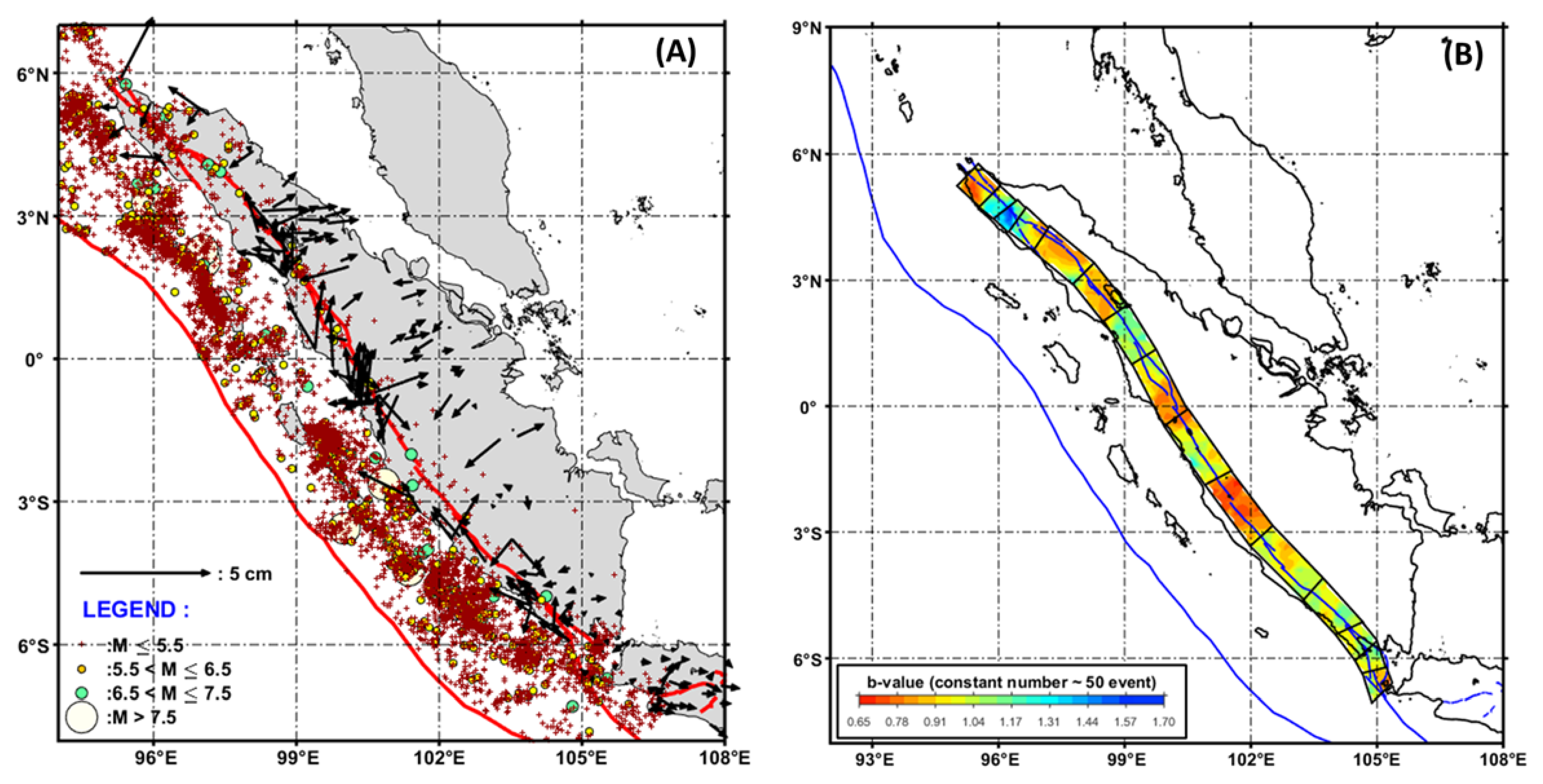
The shallow earthquake catalog data from 1963 to 2020 with Mw ≥ 4.7 and a maximum depth of 50 km [9] of 1963–2016 and GCMT catalog of 2017–2020, the active fault and pre-seismic GPS data are used in this study (Figure 2A). The active fault data are based on the newly revised [9] and recent studies [8,48]. The pre-seismic GPS data are based on [2,6,49,50,51,52,53,54]. The zonation based on the clustering study of [21] is adopted for estimating DC and the b-value. In this study, about 15 zones around SFZ are used by following their suggestion [21] to merge the zonations 15th and 16th.
First, to estimate the b-value, we grid the study area based on 15 zones around the SFZ by 10 km × 10 km. Furthermore, the b-value is calculated based on the maximum likelihood (2) using a constant number of 50 events on each grid. The result can be found in Figure 2B.
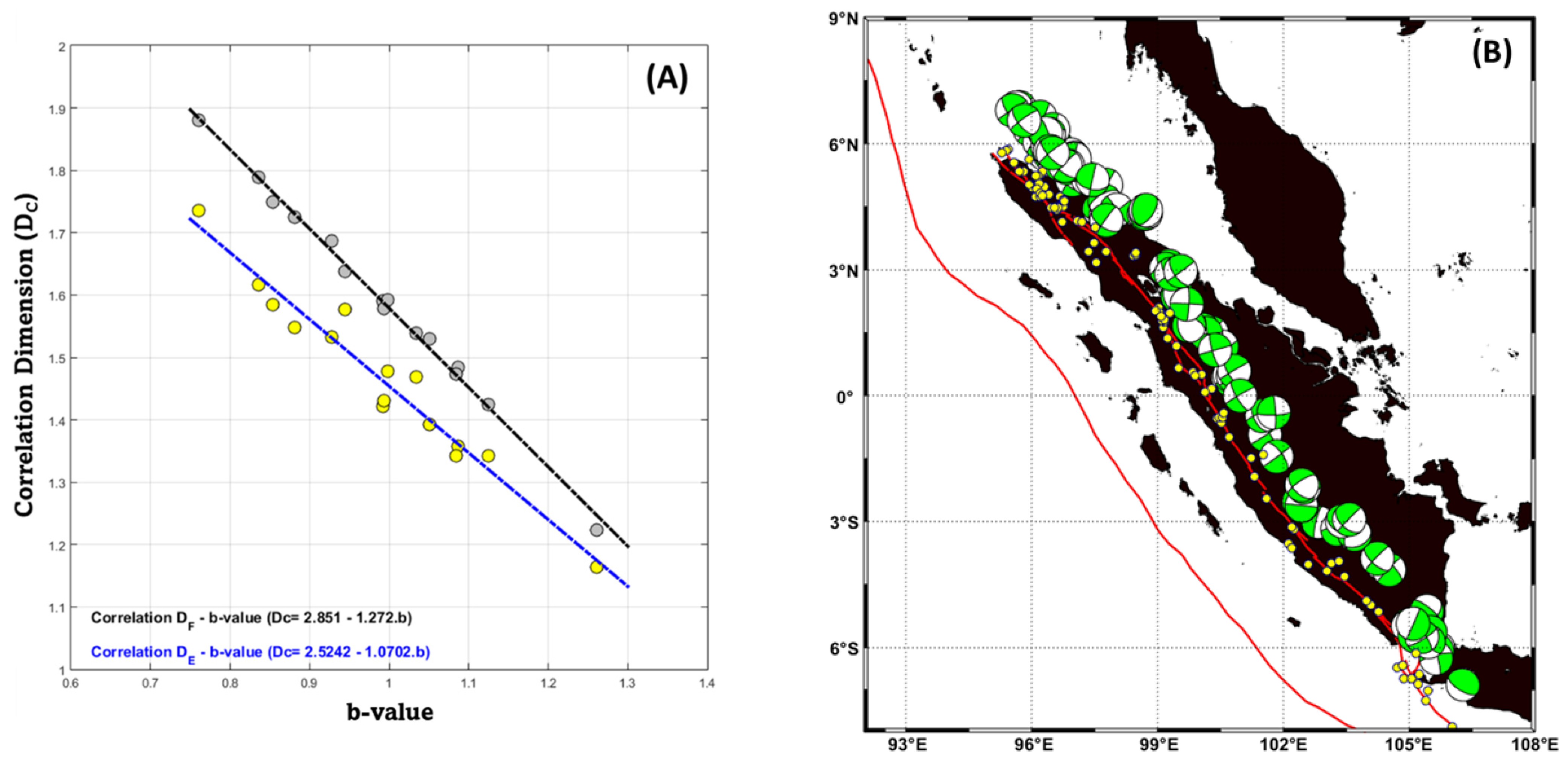
Based on the result of Figure 2B, the mean b-value of each zone is calculated, and the DE and DF are estimated using (7) based on the box-counting algorithm. Furthermore, the cross plotting between DE or DF with the mean b-value is constructed. The result can be seen in Figure 3A. In this study, the purpose of evaluating both DE and DF is to find a better correlation between the correlation dimension and the b-value utilized to estimate the SHF of the SFZ or the sites in the SFZ selected zone.
The correlation between DF, DE, and the b-value was then evaluated by referring to the previous studies [34,35,38] in which linear regression was applied. Based on Figure 3A, a reasonable correlation between two seismotectonic parameters, DF-b, and DE-b, for Sumatra Island can be found. It appears that the relationship of DF-b seems better compared to DE-b. It is probably related to the certainty of the distribution of the geometry data. The surface break of the late quaternary active fault is better than the distribution of the epicenter of the earthquake data. Next, to better understand the focal mechanism of the GCMT earthquake catalog in the depth range of 10 to 50 km around the SFZ depicts the strike-slip with a right lateral mechanism, as shown in Figure 3B.
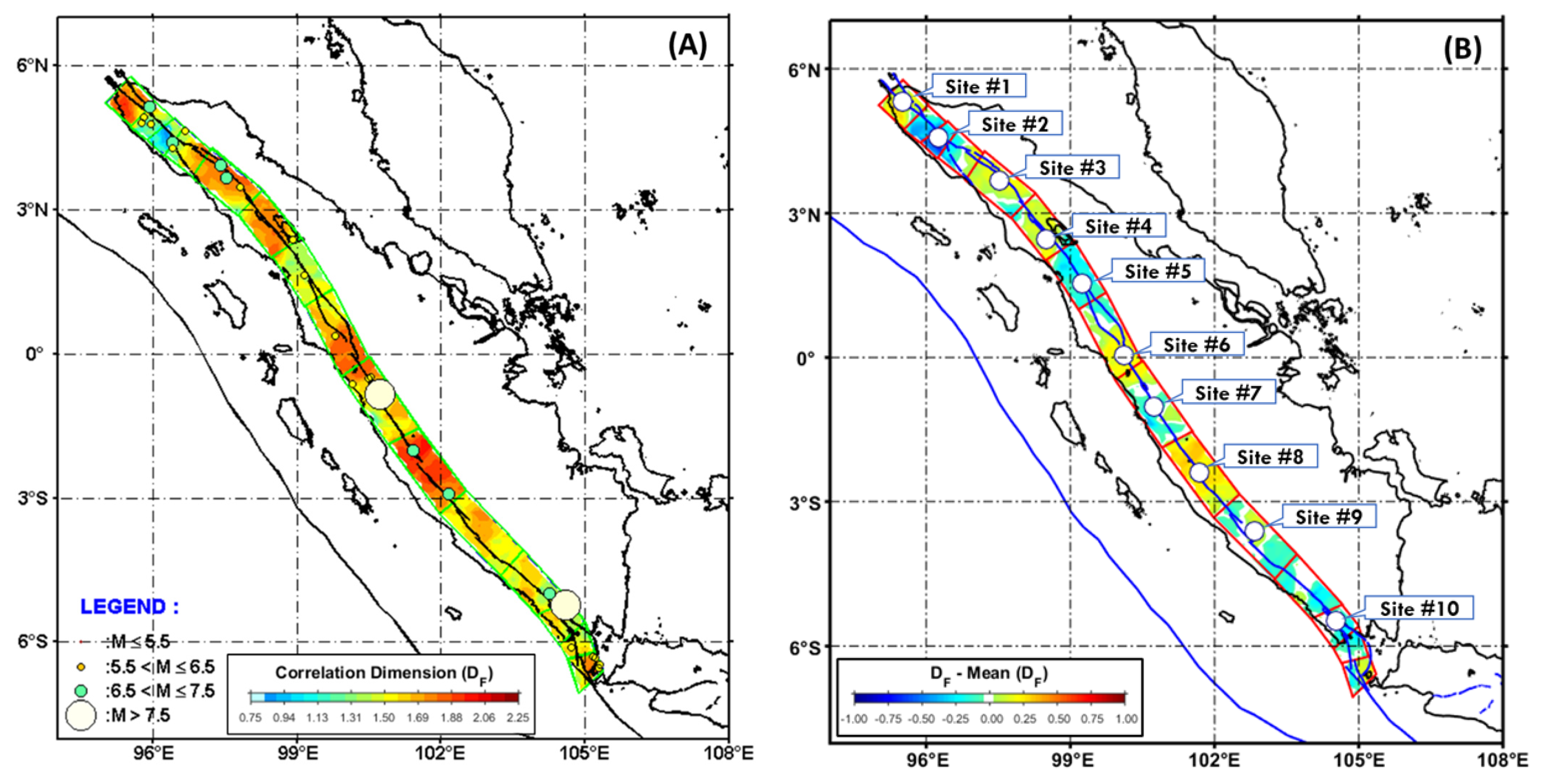
The next step calculates the DF over the entire area of the 15 zones using the equation DF = 2.851 – 1.272b with the input of the b-value map of Figure 2B. The result can be found in Figure 4A. Figure 4A shows the map of the estimated DF overlay with the historical large earthquake catalog around the SFZ. The relatively high DC coincides with the historical data of the large earthquakes with a maximum depth of less than 50 km from 1925 to 2014. To enhance the contrast of DF, we then constructed the map of DF subtracted by the mean of DF over the entire area of the 15 zones. Furthermore, we selected about ten sites to evaluate the SHF. The result can be found in Figure 4B. Referring to Figure 4B, relatively high DC (DC > the mean of DF) is distributed along zone 1, zone 5, zone 6, zone 8, zone 10, and part of zone 11; most of the previous historical large earthquakes are found.
The reliable annual seismicity rate model needs to be constructed to estimate the SHF on each site we selected. To assess the reliability of the annual seismicity rate model in this study is developed by integrating shallow earthquake catalog, active fault, and the pre-seismic GPS data. The summarized workflow in this study based on Section 2.3, Section 2.4, Section 2.5 and Section 2.6 could be described as follows. First, we smoothed the shallow earthquake catalog data around the study area using a 50 km correlation distance. Next, the synthetic catalog data model based on active fault data are smoothed using a correlation distance of 25 km. The integration between the two models was done by weighting the A-value model from the earthquake catalog with normalized smoothed seismicity obtained from active fault data. Furthermore, the shallow crustal dynamic data are incorporated in this study by following [39]; it is used GPS data.
The algorithm for constructing the model using the GPS data are as follows. First, we developed the seismic moment rate is based on Sumatran Island’s horizontal crustal strain model. In this step, the least-square prediction method [39,40,47,61,62,67] was applied to calculate the horizontal crustal strain based on each cell’s horizontal surface displacement estimation over the entire study area. Furthermore, each cell’s seismic moment could be calculated using Equation (8) [41,42,43,44]. We assumed the rigidity (μ) and the seismogenic thickness (H) to be 3.4 × 10¹¹ dyne·cm−2 and 20 km, respectively [39,40]. The result of the seismic moment rate model can be found in Figure 4A. Figure 4A shows that the areas with relatively high correlation dimensions (DF) coincide with high seismic moment loading rates, implying high tectonic stress loading that could pose the risk of producing significant earthquake hazards. The result of this study is aligned with the previous study [34,35]; however, the advantage result of this study is that we could understand the correlation between the high DC with the possible present-day strain loading since we incorporate the present-day shallow crustal movement data. It is suggested that the algorithm of this study is applicable in the other active tectonic area as far as the data are available.
Finally, the annual seismicity rate model around the SFZ is estimated based on the integrated annual A-value of an earthquake and active fault data as described in Section 2.4 and is weighted by the normalized seismic moment rate based on GPS data as is shown in Figure 5A. The result can be found in Figure 5B. Figure 5B shows the annual seismicity rate model that we propose as the most reliable model to estimate seismic hazards along SFZ. In addition, the model is suggested to have a better certainty in geometrical source and rate distribution.
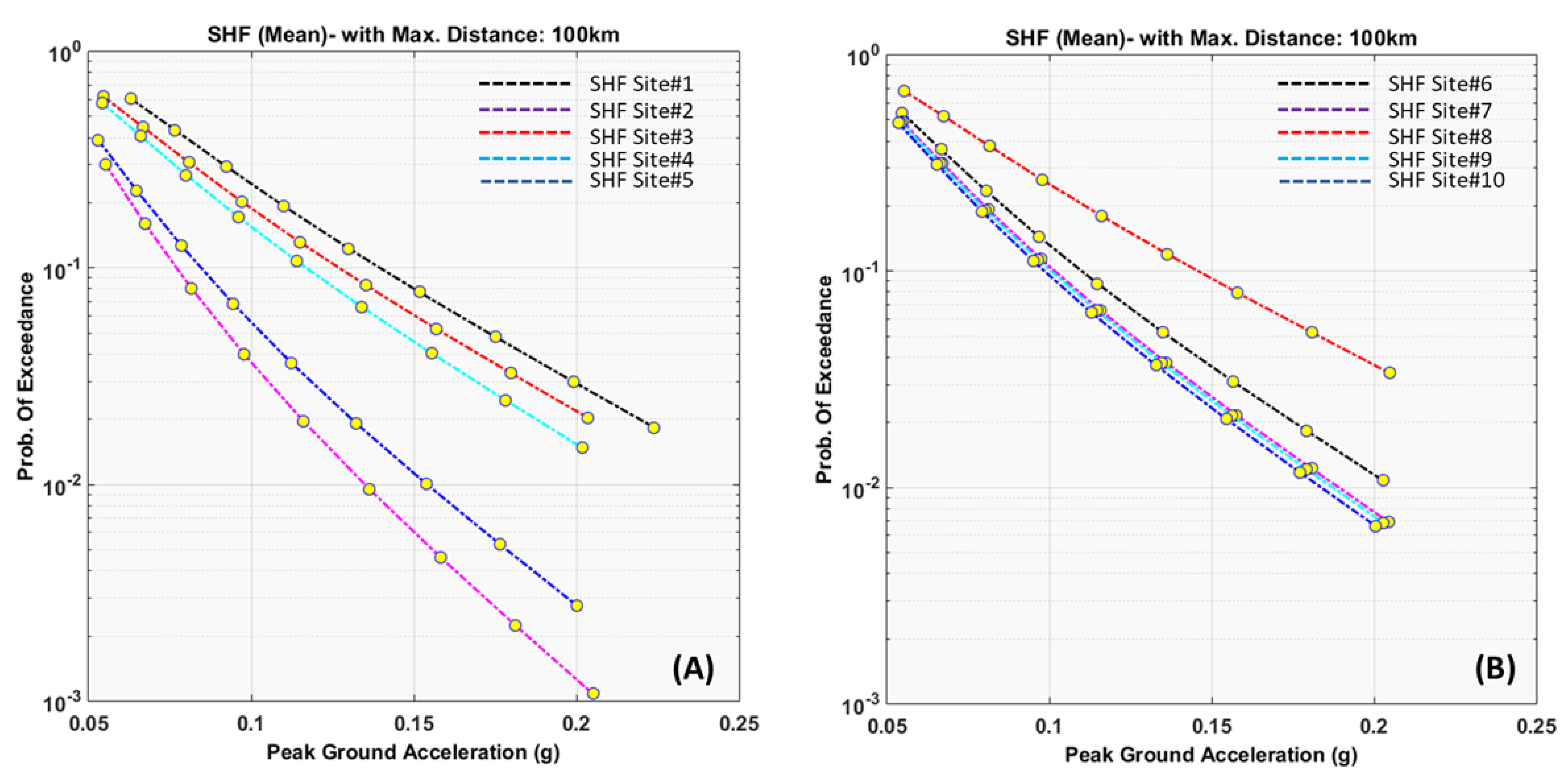
Furthermore, the SHF curve of the total probability of exceedance versus the mean of the peak ground acceleration of each observation point (sites #1 to #10) was constructed using the maximum radius distance of about 100 km with a magnitude range of 6.0–8.0. Since seismicity smoothing was used, the point source model was applied, and the source depth was placed at about half of the seismogenic thickness (about 20 km), with the starting locking depth being 5 km [39]; thus, a source depth of 15 km was used. The period of the SHF evaluation was set at about 50 years. The result of the SHF curve can be seen in Figure 6A,B. Another critical finding in this study is that the relatively high correlation dimension coincides with a high SHF curve, and it could be summarized that the areas with a relatively high correlation dimension (DF) overlap with high seismic moment loading rates, which may imply high tectonic stress loading that could pose the risk of producing significant earthquake hazards in the future.

4. Conclusions

This study could characterize a reasonable correlation between two seismotectonic parameters, DF-b and DE-b, for Sumatra Island, especially around SFZ. The relationships are DF-b and DE-b, respectively (DF = 2.851 − 1.272b) and (DE = 2.5242 − 1.0702b). It is found that the relationship of DF-b seems better compared to DE-b. The result leads to the fundamental understanding that the certainty of the source geometry distribution based on the surface break of the late quaternary active fault is better than the distribution of the epicenter of the earthquake data.
The correlation dimension map in this study concludes that the relatively high DC coincides with the historical data of large earthquakes from 1925 to 2014. The most critical finding in this study is that the areas with relatively high DC coincide with high seismic moment loading rates, implying high tectonic stress loading that could pose the risk of producing significant earthquake hazards in the future. The advantage of this study compared to the previous research is that we could understand the correlation between the high DC with the possible present-day strain loading since we incorporate the present-day shallow crustal dynamic data.
In this study, we have proposed the algorithm to construct the most reliable annual seismicity rate model along the SFZ. The model is estimated based on the integrated annual A-value of the shallow earthquake, active fault, and seismic moment rate derived from the GPS data. We suggest that the annual seismicity rate model tends to have better certainty in geometrical source and rate distribution.
Another critical finding of this study leads us to conclude that the relatively high correlation dimension coincides with a high SHF curve. Therefore, it could be summarized that the areas with relatively high DC overlap with high seismic moment loading rates, which may imply high tectonic stress loading that could pose the risk of producing significant earthquake hazards in the future. This study also led us to the understanding that the high correlation dimension is closely related to the possibility of high seismic hazards in the future.

Supplementary Materials

The following supporting information can be downloaded at: https://www.mdpi.com/article/10.3390/geohazards3020012/s1, They contain shallow earthquake catalog data (combined of PUSGEN catalog of 1963–2016 and GCMT catalog of 2017–2020), estimated b-value based on a constant number of 50 events, the boundary zone based on Ref. [21], and grid in MAT file format, LSQR GPS data, active fault data of SFZ and other materials related to the estimation results in this manuscript.

Author Contributions

W.T. developed the main idea and algorithm, analysed, and prepared the figures and the manuscript. D.A.S. helped to collect the GPS data based on several manuscripts. D.P.S. and S.S. helped in the manuscript preparation and discussion. Finally, D.H.N. helped support the most recent active fault data of Sumatra Island and in the discussion. All authors have read and agreed to the published version of the manuscript.

Funding

Funding was supported in part by the Institute of Research and Community Services (LPPM), Bandung Institute of Technology (ITB), Indonesia.

Institutional Review Board Statement

Not applicable.

Informed Consent Statement

Not Applicable.

Data Availability Statement

The authors declare that the materials and data used in this manuscript will be made available promptly to the Editorial Board Members and Referees upon request. The earthquake catalog and historical data are based on the PUSGEN2017 [9] and GCMT of 2017 to 2020 catalog, public domain data. The active fault data are based on the newly revised PUSGEN 2017 and recent studies [8,48]. The pre-seismic GPS data are based on the studies of [2,49,50,51,52,53,54].

Acknowledgments

The authors wish to thank the Global Geophysics Group and the Faculty of Mining and Petroleum Engineering, Bandung Institute of Technology, for their help in publishing this paper.

Conflicts of Interest

The authors declare that they have no competing interests.

References

  1. Fitch, T.J. Plate convergence, transcurrent faults, and internal deformation adjacent to southeast Asia and the western Pacific. J. Geophys. Res. 1972, 77, 4432–4460. [Google Scholar] [CrossRef]
  2. Prawirodirdjo, L.; McCaffrey, R.; Chadwell, C.D.; Bock, Y.; Subarya, C. Geodetic observations of an earthquake cycle at the Sumatra subduction zone: Role of interseismic strain segmentation. J. Geophys. Res. Solid Earth 2010, 115, B03414. [Google Scholar] [CrossRef] [Green Version]
  3. Sieh, K.; Natawidjaja, D.H. Neotectonics of the Sumatran fault, Indonesia. J. Geophys. Res. 2000, 105, 28295–28326. [Google Scholar] [CrossRef] [Green Version]
  4. Genrich, J.F.; Bock, Y.; McCaffrey, R.; Prawirodirdjo, L.; Stevens, C.W.; Puntodewo, S.S.O. Distribution of slip at the northern Sumatran fault system. J. Geophys. Res. 2000, 105, 28327–28341. [Google Scholar] [CrossRef]
  5. McCaffrey, R. Slip vectors and stretching of the Sumatran forearc. Geology 1991, 19, 881–884. [Google Scholar] [CrossRef]
  6. Bradley, K.E.; Feng, L.; Hill, E.M.; Natawidjaja, D.H.; Sieh, K. Implications of the diffuse deformation of the Indian Ocean lithosphere for slip partitioning of oblique plate convergence in Sumatra. J Geophys. Res. Solid Earth 2017, 122, 572–591. [Google Scholar] [CrossRef] [Green Version]
  7. Natawidjaja, D.H.; Triyoso, W. The Sumatran fault zone—From source to hazard. J. Earthq. Tsunami 2007, 1, 21–47. [Google Scholar] [CrossRef]
  8. Natawidjaja, D.H. Updating active fault maps and slip rates along the Sumatran Fault Zone, Indonesia. IOP. Conf. Ser. Earth Environ. Sci. 2018, 118, 012001. [Google Scholar] [CrossRef] [Green Version]
  9. Tim Pusat Studi Gempa Nasional-2017 (The 2017 PuSGen). Peta Sumber dan Bahaya Gempa Indonesia Tahun 2017; Kementrian Pekerjaan Umum dan Perumahan Rakyat: Jakarta, Indonesia, 2017. (In Indonesian) [Google Scholar]
  10. McCloskey, J.T.; Nalbant, S.S.; Steacy, S. Earthquake risk from co-seismic stress. Nature 2005, 434, 291. [Google Scholar] [CrossRef]
  11. Qiu, Q.; Chan, C.-H. Coulomb stress perturbation after great earthquakes in the Sumatran subduction zone: Potential impacts in the surrounding region. J. Southeast Asian Earth Sci. 2019, 180, 103869. [Google Scholar] [CrossRef]
  12. Cattin, R.; Chamot-Rooke, N.; Pubellier, M.; Rabaute, A.; Delescluse, M.; Vigny, C.; Fleitout, L.; Dubernet, P. Stress change and effective friction coefficient along the Sumatra-Andaman-Sagaing fault system after the 26 December 2004 (Mw= 9.2) and the 28 March 2005 (Mw= 8.7) earthquakes. Geochem. Geophys. Geosystems 2009, 10, 1–22. [Google Scholar] [CrossRef] [Green Version]
  13. Visini, F.; Valentini, A.; Chartier, T.; Scotti, O.; Pace, B. Computational Tools for Relaxing the Fault Segmentation in Probabilistic Seismic Hazard Modelling in Complex Fault Systems. Pure Appl. Geophys. 2019, 177, 1855–1877. [Google Scholar] [CrossRef]
  14. Swan, F.H.; Schwartz, D.P.; Cluff, L.S. Recurrence of moderate to large magnitude earthquakes produced by surface faulting on the Wasatch Fault Zone, Utah. Bull. Seismol. Soc. Am. 1980, 70, 1431–1462. [Google Scholar]
  15. Schwartz, D.P.; Coppersmith, K.J. Fault behavior and characteristic earthquakes: Examples from the Wasatch and San Andreas Fault Zones. J. Geophys. Res. Earth Surf. 1984, 89, 5681–5698. [Google Scholar] [CrossRef]
  16. King, G.; Nabelek, J. Role of fault bends in the initiation and termination of earthquake rupture. Science 1985, 228, 984–987. [Google Scholar] [CrossRef] [PubMed]
  17. Meng, L.; Ampuero, J.P.; Stock, J.; Duputel, Z.; Luo, Y.; Tsai, V.C. Earthquake in a Maze: Compressional Rupture Branching During the 2012 Mw 8.6 Sumatra Earthquake. Science 2012, 337, 724–726. [Google Scholar] [CrossRef]
  18. Field, E.H.; Dawson, T.E.; Felzer, K.R.; Frankel, A.D.; Gupta, V.; Jordan, T.H.; Parsons, T.; Petersen, M.D.; Stein, R.S.; Weldon, R.J.; et al. Uniform California Earthquake Rupture Forecast, Version 2 (UCERF 2). Bull. Seism. Soc. Am. 2009, 99, 2053–2107. [Google Scholar] [CrossRef] [Green Version]
  19. Stirling, M.; McVerry, G.; Gerstenberger, M.; Litchfield, N.; Van Dissen, R.; Berryman, K.; Barnes, P.; Wallace, L.; Villamor, P.; Langridge, R.; et al. National Seismic Hazard Model for New Zealand: 2010 Update. Bull. Seism. Soc. Am. 2012, 102, 1514–1542. [Google Scholar] [CrossRef] [Green Version]
  20. Peruzza, L.; Pace, B.; Visini, F. Fault-based earthquake rupture forecast in Central Italy: Remarks after the L’Aquila Mw 6.3 Event. Bull. Seism. Soc. Am. 2011, 101, 404–412. [Google Scholar] [CrossRef]
  21. Burton, P.W.; Hall, T.R. Segmentation of the Sumatran fault. Geophys. Res. Lett. 2014, 41, 4149–4158. [Google Scholar] [CrossRef] [Green Version]
  22. Segall, P.; Pollard, D.D. Mechanics of discontinuous faults. J. Geophys. Res. 1980, 85, 4337–4350. [Google Scholar] [CrossRef]
  23. Wesnousky, S.G. Predicting the endpoints of earthquake ruptures. Nature 2006, 444, 358–360. [Google Scholar] [CrossRef] [PubMed]
  24. Petersen, M.D.; Dewey, J.; Hartzell, S.; Mueller, C.; Harmsen, S.; Frankel, A.; Rukstales, K. Probabilistic seismic hazard analysis for Sumatra, Indonesia and across the Southern Malaysian Peninsula. Tectonophysics 2004, 390, 141–158. [Google Scholar] [CrossRef]
  25. Mandelbrot, B.B. The Fractal Geometry of Nature; Freeman Press: San Francisco, CA, USA, 1982. [Google Scholar]
  26. Hirata, T. Correlation between the b-value and the fractal dimension of earthquakes. J. Geophys. Res. 1989, 94, 7507–7514. [Google Scholar] [CrossRef]
  27. Henderson, J.; Main, I.G.; Meredith, P.G.; Sammonds, P.R. The evolution of seismicity-observation, experiment, and a fracture—Mechanical interpretation. J. Struct. Geol. 1992, 14, 905–913. [Google Scholar] [CrossRef]
  28. Öncel, A.O.; Alptekin, Ö.; Main, I. Temporal variations of the fractal properties of seismicity in the western part of the north Anatolian fault zone: Possible artifacts due to improvements in station coverage. Nonlinear Process. Geophys. 1995, 2, 147–157. [Google Scholar] [CrossRef] [Green Version]
  29. Oncel, A.O.; Wilson, T. Anomalous seismicity preceding the 1999 Izmit event, NW Turkey. Geophys. J. Int. 2007, 169, 259–270. [Google Scholar] [CrossRef] [Green Version]
  30. Sukmono, S.; Zen, M.T.; Kadir, W.G.A.; Hendrajaya, L.; Santoso, D.; Dubois, J. Fractal pattern of the Sumatra fault seismicity and its possible application to earthquake prediction. Bull. Seismol. Soc. Am. 1997, 87, 1685–1690. [Google Scholar] [CrossRef]
  31. Sukmono, S.; Zen, M.T.; Kadir, W.G.A.; Hendrajaya, L.; Santoso, D.; Dubois, J. Fractal geometry of the Sumatra active fault system and its geodynamical implications. J. Geodyn. 1996, 22, 1–9. [Google Scholar] [CrossRef]
  32. Caneva, A.; Smirnov, V. Using the Fractal Dimension of Earthquake Distributions and Slope of the Recurrence Curve to Forecast Earthquakes in Colombia. Earth Sci. Res. J. 2004, 8, 3–9. [Google Scholar]
  33. Roy, S.; Ghosh, U.; Hazra, S.; Kayal, J.R. Fractal dimension and b-value mapping in the Andaman-Sumatra subduction zone. Nat. Hazards 2011, 57, 27–37. [Google Scholar] [CrossRef]
  34. Pailoplee, S.; Choowong, M. Earthquake frequency-magnitude distribution and fractal dimension in mainland Southeast Asia. Earth Planets Space 2014, 66, 8. [Google Scholar] [CrossRef] [Green Version]
  35. Goebell, T.H.W.; Kwiatek, G.; Becker, T.W.; Brodsky, E.E.; Dresen, G. What allows seismic events to grow big?: Insights from b-value and fault roughness analysis in laboratory stick-slip experiments. Geology 2017, 45, 815–818. [Google Scholar] [CrossRef] [Green Version]
  36. Wyss, M.; Sammis, C.G.; Nadeau, R.M.; Wiemer, S. Fractal Dimension and b-Value on Creeping and Locked Patches of the San Andreas Fault near Parkfield, California. Bull. Seism. Soc. Am. 2004, 94, 410–421. [Google Scholar] [CrossRef]
  37. Gutenberg, R.; Richter, C.F. Frequency of earthquakes in California. Bull. Seism. Soc. Am. 1944, 34, 185–188. [Google Scholar] [CrossRef]
  38. Bayrak, Y.; Ozturk, S. Spatial and temporal variations of the aftershock sequences of the 1999 İzmit and Düzce earthquakes. Earth Planets Space 2004, 56, 933–944. [Google Scholar] [CrossRef] [Green Version]
  39. Triyoso, W.; Suwondo, A.; Yudistira, T.; Sahara, D.P. Seismic Hazard Function (SHF) study of coastal sources of Sumatra Island: SHF evaluation of Padang and Bengkulu cities. Geosci. Lett. 2020, 7, 1–7. [Google Scholar] [CrossRef]
  40. Triyoso, W.; Sahara, D.P. Seismic hazard function mapping using estimated horizontal crustal strain off West Coast Northern Sumatra. Front. Earth Sci. 2021, 9, 1–11. [Google Scholar] [CrossRef]
  41. Ward, S.N. A multidisciplinary approach to seismic hazard in southern California. Bull. Seism. Soc. Am. 1994, 84, 1293–1309. [Google Scholar] [CrossRef]
  42. Molnar, P. Earthquake recurrence intervals and plate tectonics. Bull. Seism. Soc. Am. 1979, 69, 115–133. [Google Scholar] [CrossRef]
  43. Savage, J.C.; Simpson, R.W. Surface strain accumulation and the seismic moment tensor. Bull. Seism. Soc. Am. 1997, 87, 1345–1353. [Google Scholar] [CrossRef]
  44. Field, E.H.; Jackson, D.D.; Dolan, J.F. A mutually consistent seismic-hazard source model for southern California. Bull. Seism. Soc. Am. 1999, 89, 559–578. [Google Scholar]
  45. Scholz, C.H. The frequency-magnitude relation of microfracturing in rock and its relation to earthquakes. Bull. Seism. Soc. Am. 1968, 58, 399–415. [Google Scholar] [CrossRef]
  46. Frankel, A. Mapping Seismic Hazard in the Central and Eastern United States. Seism. Res. Lett. 1995, 66, 8–21. [Google Scholar]
  47. Triyoso, W.; Shimazaki, K. Testing various seismic potential models for hazard estimation against a historical earthquake catalog in Japan. Earth Planets Space 2012, 64, 673–681. [Google Scholar] [CrossRef] [Green Version]
  48. Natawidjaja, D.H.; Bradley, K.; Daryono, M.R.; Aribowo, S.; Herrin, J. Late Quaternary eruption of the Ranau Caldera and new geological slip rates of the Sumatran Fault Zone in Southern Sumatra, Indonesia. Geosci. Lett. 2017, 4, 21. [Google Scholar] [CrossRef] [Green Version]
  49. Bird, P. An updated digital model of plate boundaries. Geochem. Geophys. Geosyst. 2003, 4, 1027. [Google Scholar] [CrossRef]
  50. Chlieh, M.; Avouac, J.-P.; Hjorleifsdottir, V.; Song, T.-R.A.; Ji, C.; Sieh, K.; Sladen, A.; Hebert, H.; Prawirodirdjo, L.; Bock, Y.; et al. Coseismic Slip and Afterslip of the Great Mw 9.15 Sumatra-Andaman Earthquake of 2004. Bull. Seism. Soc. Am. 2007, 97, S152–S173. [Google Scholar] [CrossRef] [Green Version]
  51. Shearer, P.; Bürgmann, R. Lessons Learned from the 2004 Sumatra-Andaman Megathrust Rupture. Annu. Rev. Earth Planet. Sci. 2010, 38, 103–131. [Google Scholar] [CrossRef] [Green Version]
  52. Susilo; Meilano, I.; Abidin, H.Z.; Sapie, B.; Efendi, J.; Wijanarto, A.B. Preliminary Results of Indonesian Strain Map Based on Geodetic Measuremnts. AIP Conf. Proc. 2016, 1730, 040004. [Google Scholar] [CrossRef]
  53. Khaerani, D.; Meilano, I.; Sarsito, D.A.; Susilo, D. Deformation of West Sumatra Due to the 2016 Earthquake (M7.8) Based on Continuous GPS Data. In Proceedings of the 2018 IEEE Asia-Pacific Conference on Geoscience, Electronics and Remote Sensing Technology (AGERS), Jakarta, Indonesia, 18–19 September 2018. [Google Scholar]
  54. Qiu, Q.; Feng, L.; Hermawan, I.; Hill, E.M. Coseismic and Postseismic Slip of the 2005 Mw 8.6 Nias-Simeulue Earthquake: Spatial Overlap and Localized Viscoelastic Flow. J. Geophys. Res. Solid Earth 2019, 124, 7445–7460. [Google Scholar] [CrossRef] [Green Version]
  55. Frohlich, C.; Davis, S. Teleseismic b-values: Or, much ado about 1.0. J. Geophys. Res. 1993, 98, 631–644. [Google Scholar] [CrossRef]
  56. Aki, K. Maximum likelihood estimate of b in the formula log N = a bM and its confidence limits. Bull. Earthq. Res. Inst. Tokyo Univ. 1965, 43, 237–239. [Google Scholar]
  57. Grassberger, P.; Procaccia, I. Measuring the strangeness of strange attractors. Physica 1983, D9, 189–208. [Google Scholar]
  58. Popescu, A.L.; Popescu, D.; Ionescu, R.T.; Angelescu, N.; Romeo Cojocaru, R. Efficient fractal method for texture classification. In Proceedings of the 2nd International Conference on Systems and Computer Science (ICSCS), Villeneuve d’Ascq, France, 26–27 August 2013. [Google Scholar] [CrossRef]
  59. Bender, B. Maximum likelihood estimation of b values for magnitude grouped data. Bull. Seism. Soc. Am. 1983, 73, 831–851. [Google Scholar] [CrossRef]
  60. Triyoso, W.; Suwondo, A.; Naibaho, Z.Y.X. Earthquake Potential Hazard Analysis of Palembang City, Sumatra Island. Indones. J. Geosci. 2020, 8, 1–9. [Google Scholar] [CrossRef]
  61. El-Fiky, G.S.A.; Kato, T. Continuous distribution of the horizontal strain in the Tohoku district, Japan, predicted by least-squares collocation. Geodynamics 1999, 27, 213–236. [Google Scholar] [CrossRef]
  62. El-Fiky, G.S.; Kato, T.; Oware, E.N. Crustal deformation and interplate coupling in the Shikoku district, Japan, as seen from continuous GPS observation. Tectonophysics 1999, 314, 387–399. [Google Scholar] [CrossRef]
  63. Fukushima, Y.; Tanaka, T. Reply to T. Masuda and M. Ohtake’s “Comment on ‘A new attenuation relation for peak horizontal acceleration of strong earthquake ground motion in Japan’”. Bull. Seism. Soc. Am. 1992, 82, 523. [Google Scholar] [CrossRef]
  64. Fukushima, Y.; Tanaka, H. The revision of “A new attenuation relation for peak horizontal acceleration of strong earthquake ground motion in Japan”. Abstr. Seismol. Soc. Jpn. 1992, B18, 116. (In Japanese) [Google Scholar]
  65. Dziewonski, A.M.; Chou, T.-A.; Woodhouse, J.H. Determination of earthquake source parameters from waveform data for studies of global and regional seismicity. J. Geophys. Res. Earth Surf. 1981, 86, 2825–2852. [Google Scholar] [CrossRef]
  66. Ekström, G.; Nettles, M.; Dziewoński, A. The global CMT project 2004–2010: Centroid-moment tensors for 13,017 earthquakes. Phys. Earth Planet. Inter. 2012, 200–201, 1–9. [Google Scholar] [CrossRef]
  67. Kato, T.; El-Fiky, G.S.; Oware, E.N.; Miyazaki, S. Crustal strains in the Japanese Islands as deduced from dense GPS array. Geophys. Res. Lett. 1998, 25, 3445–3448. [Google Scholar] [CrossRef]
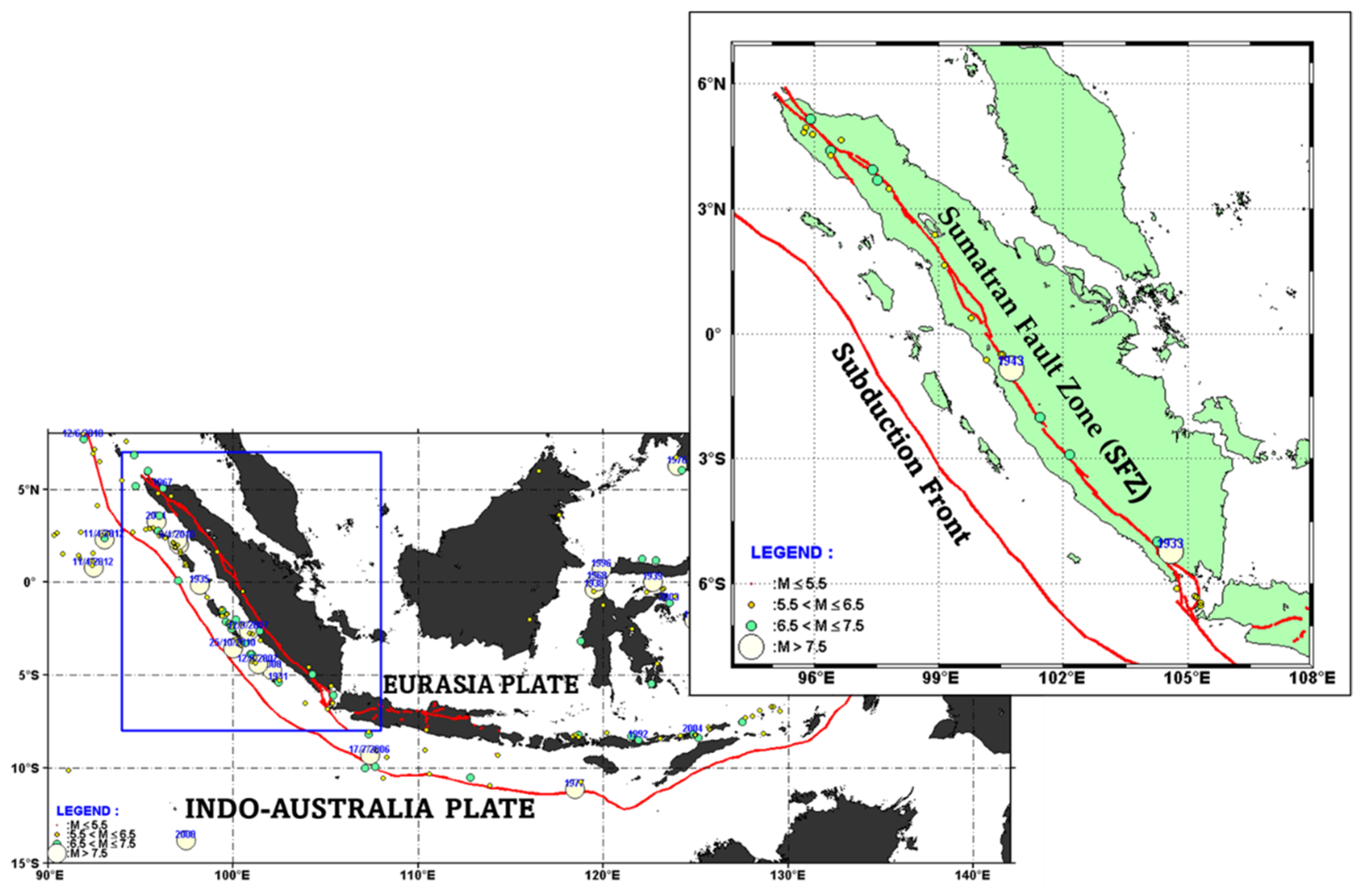
Figure 1. The Sumatran seismotectonic map depicting the Sumatran Subduction Zone and Sumatran Fault Zone (SFZ) overlays with the historical shallow large earthquake data of 1925–2014 with a magnitude (Mw) larger than or equal to 6.0. Historical earthquake data are based on Ref. [9].
Geohazards 03 00012 g001
Figure 2. The shallow earthquake catalog data from 1963 to 2020 with the magnitude of Mw ≥ 4.7 and a maximum depth of 50 km [9] of 1963–2016 and the GCMT catalog of 2017–2020, the active fault, and pre-seismic GPS data (A). The b-value map overlays with the 15 zones area (B). The b-value is estimated based on the maximum likelihood (2) using a constant number of 50 events on each grid.
Geohazards 03 00012 g002
Figure 3. The cross-plot DF, DE, and the mean b-values are estimated based on the 15 zones (A). The focal mechanism plot is based on the GCMT catalog of shallow earthquake data for earthquakes at depths less than or equal to 50 km with a magnitude larger than or equal to 4.7 in the earthquake period between January 1976 to December 2020 [65,66] (B).
Geohazards 03 00012 g003
Figure 4. The map of DF overlay with the historical earthquake catalog with the Mw ≥ 6.0 around the SFZ (A). DF is calculated using equation DF = 2.851 – 1.272b with the input of the b-value map of Figure 2B. The map of (DF—mean of DF) over the entire clustered zone boundary of Burton and Hall [21] and selected about ten sites to evaluate the SHF starting from the North-West to South-East (B). The relatively high DC coincides with the historical shallow large earthquakes data of Ref. [9] from 1925 to 2014.
Geohazards 03 00012 g004
Figure 5. The estimated seismic moment rate is based on the horizontal crustal strain model around Sumatra Island (A). The annual seismic rate model for the SHF calculation was constructed based on the seismic smoothing of the earthquake catalog weighted by the normalized fault seismic model and the normalized seismic moment rate model based on the GPS data (B).
Geohazards 03 00012 g005
Figure 6. The graphs show the SHF curve of each observation point (A,B). The SHF curve of total probability of exceedance versus the mean of the peak ground acceleration of each observation point (sites #1 to #10) was constructed using the maximum radius distance of about 100 km with a magnitude range of 6.0–8.0. The source depth was set at half of the seismogenic thickness, which was about 20 km, and the starting locking depth of 5 km was used; thus, 15 km of the source depth was used. The period of the SHF evaluation was set at about 50 years.
Geohazards 03 00012 g006
Publisher’s Note: MDPI stays neutral with regard to jurisdictional claims in published maps and institutional affiliations.