Mathematical Modeling and Solution of the Moving-Boundary Problem Related to Substrate Diffusion and Reaction in Enzymatic Catalytic Particles

Abstract

This study presents a transient mathematical model and its numerical solution for the moving-boundary problem related to substrate diffusion and reaction in enzymatic catalytic particles. The main focus is on bioreactor startup, where the initial substrate concentration inside the particles is zero, forming a dead core that shrinks over time and makes the catalytic effectiveness factor time-dependent. The substrate mass balance leads to a partial differential equation with a moving boundary, solved using the method of lines coupled with Newton’s method (MLN), implemented in Wolfram Mathematica (WM). The proposed approach was validated for zero- and first-order kinetics at steady state, whose analytical solutions are available. Compared to the method of orthogonal collocation on finite elements, the MLN offers advantages such as not requiring an initial concentration profile and simple implementation in WM. The results demonstrate that the proposed method provides accurate and physically consistent solutions, contributing to a better understanding of dead-core dynamics and supporting the design of heterogeneous bioreactors with immobilized enzymes.

1. Introduction

The development of bioprocesses involving cells and enzymes encompasses the production of new materials, improvements in product quality, minimization of environmental impacts, and overall cost reduction [1,2,3,4,5]. In these processes, cells and enzymes convert raw materials (substrates) into products inside bioreactors, and the selection of the appropriate operation mode requires an evaluation of the advantages and limitations associated with each configuration [6,7,8].

Immobilized enzymes are widely employed in industrial processes for the production of pharmaceuticals, chemicals, food and beverages, biofuels, and other biotechnological products [9,10,11]. The use of free enzymes in continuous reactors generally leads to biocatalyst loss at the reactor outlet. Since enzyme cost is a major constraint in industrial applications, immobilizing enzymes on solid supports can significantly reduce overall process expenses, as catalyst separation and reuse are simpler than in systems with free enzymes [7,12]. These advantages have increased the use of heterogeneous enzymatic reactors [13,14].

Mathematical models are essential for the design, optimization, and control of heterogeneous biocatalytic reactors. These models are commonly based on simplifying assumptions, such as isothermal operation, negligible external diffusional resistance at the particle surface, and uniform catalyst properties [15,16,17,18]. Under some operating conditions, the heterogeneous nature of immobilized systems may lead to significant substrate diffusion limitations within the particle, resulting in the formation of a time-dependent dead core, whose evolution can be described by classical diffusion–reaction models [16,17,18,19].

Modeling the startup of heterogeneous enzymatic reactors requires the transient description of substrate concentration profiles inside the particles. This transient analysis is crucial to estimate the duration of the startup period and also to determine the catalytic effectiveness factor at both transient and stationary periods [20,21,22].

The time-dependent diffusion–reaction process in biocatalyst particles is governed by a nonlinear partial differential equation. Since many nonlinear or partially linear differential equations do not admit analytical solutions, alternative approaches are required, such as numerical methods [18,21,22,23,24,25,26,27], approximate analytical techniques [16,20,28,29,30,31,32,33,34], and artificial intelligence-based methods [35,36,37,38,39]. Among these, numerical methods have been reported as the most accurate and are frequently used as reference solutions for evaluating alternative methodologies with lower computational effort [16,18].

In this context, the present study proposes a numerical methodology to analyze dead-core shrinkage in biocatalyst particles in which occur enzymatic reactions governed by Michaelis–Menten (MM) kinetics. The Method of Lines coupled with Newton’s method (MLN) is employed to solve the governing partial differential equation describing combined diffusion and reaction processes inside the particle. To evaluate the performance of the numerical methodology, simplified forms of the MM kinetics, corresponding to zero-order and first-order kinetics, are initially considered. For these simplified kinetics, analytical steady-state solutions are available for the three classical particle geometries (slab, cylindrical, and spherical), enabling direct comparison with the numerical results. Once validated, the proposed method is further compared with the approach using the method of orthogonal collocation on finite elements under steady-state conditions.

The methodology presented here enables accurate and efficient analysis of both transient and steady-state regimes for various particle geometries, providing a modeling framework whose applicability can be guided by the reactor’s operational strategy, particularly in situations where startup and other transient conditions are relevant to reactor design and performance assessment.

2. Methods

2.1. Dead-Core Shrinkage Representation

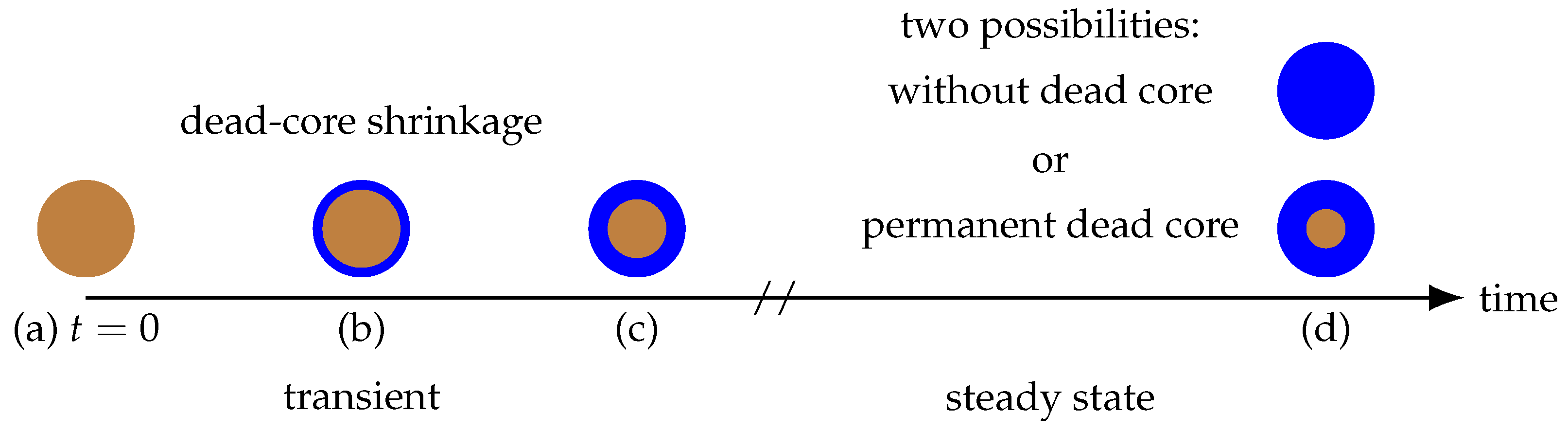
Figure 1 illustrates the transient substrate diffusion and enzymatic consumption inside a spherical biocatalyst particle, which may lead to the formation of a permanent dead core depending on the reaction and mass transport rates.

In Figure 1, the blue region denotes zones where the substrate concentration ($C_S$) is strictly greater than zero ($C_S>0$), while the brown region identifies the domain that does not contain substrate ($C_S=0$), in which reaction cannot proceed due to the absence of this reagent, here defined as the “dead core” [18,40]. At time $t=0$, before substrate addition to the bioreactor, the concentration within the immobilized-enzyme particles is zero (Figure 1a). After substrate is fed, it diffuses into the particle while being simultaneously consumed by the enzymatic reaction, leading to a moving interface that may delimit a dead core (Figure 1b,c). Once steady state is reached, two outcomes are possible: (i) diffusion is sufficient to sustain $C_S>0$ across the entire particle, yielding a “steady state without dead core” or (ii) diffusion is insufficient to overcome consumption, and a “permanent dead core”, where $C_S=0$ persists (Figure 1d).

2.2. Chemical Kinetics and the Michaelis–Menten Equation

For the accurate design of enzymatic reactors, it is necessary to know how the reaction rate is influenced by reaction conditions such as substrate, product, and enzyme concentrations. In the case of enzymes immobilized on supports, in addition to the variables already mentioned, other inherent variables from heterogeneous catalytic systems, related to external and internal transport phenomena to the particle, must be considered [41].

The derivation of a rate equation for an enzymatic reaction follows the principles of chemical kinetics. Firstly, a mechanism composed by a series of elementary steps is proposed for the reaction considered. Secondly, from key assumptions, a rate equation is derived, which is validated with kinetic data from the reaction obtained free from mass transfer effects to ensure that the measured reaction rate exclusively reflects the chemical kinetics, providing intrinsic rather than apparent kinetic parameters.

There are two different approaches to derive the Michaelis–Menten rate equation: one based on the hypothesis of rapid equilibrium and the other based on the hypothesis of pseudo-steady state [41,42]. For both hypotheses, the general mechanism for the simple enzymatic reaction $\mathrm{S}\stackrel{\mathrm{E}}{\to }\mathrm{P}$ consists of the binding of the substrate to the enzyme, forming an intermediate complex that subsequently decomposes, generating product by modifying the substrate at the enzyme’s active site and regenerating the enzyme, according to Equation (1), where $k_1$, $k_2$, and $k_3$ are the rate constants of the respective reactions.

$$\mathrm{S}+\mathrm{E}\underset{k_2}{\overset{k_1}{\rightleftharpoons }}\mathrm{ES}\stackrel{k_3}{\to }\mathrm{P}+\mathrm{E}$$

(1)

The rapid equilibrium hypothesis assumes the establishment of an equilibrium between $\mathrm{E}$, $\mathrm{S}$, and $\mathrm{ES}$, which implies that the rates of formation of the $\mathrm{ES}$ complex and its decomposition into $\mathrm{S}$ and $\mathrm{E}$ are much greater than the rate of decomposition into $\mathrm{E}$ and $\mathrm{P}$. In turn, the pseudo-steady-state hypothesis assumes that after a very brief initial transient state, a pseudo-steady state is reached for the $\mathrm{ES}$ concentration. Thus, for both approaches, it is clear that the second reaction of the scheme is the controlling step of the overall reaction rate (v), given by Equation (2):

$$v={\displaystyle \frac{d{C}_P}{dt}}=-{\displaystyle \frac{d{C}_S}{dt}}=k_3{C}_{ES}$$

(2)

In Equation (2): v is the reaction rate, $C_P$ is the product concentration, t is the time, $C_S$ is the substrate concentration, and $C_{ES}$ is the concentration of enzyme–substrate complex.

The chemical equilibrium constant (K) for the formation of the $\mathrm{ES}$ complex is given by Equation (3), where $C_{E_0}$ is the total enzyme concentration and $C_E$ is the free enzyme concentration.

$$K={\displaystyle \frac{C_{ES}}{C_S·C_E}}={\displaystyle \frac{C_{ES}}{C_S\left(C_{E_0}-C_E\right)}}={\displaystyle \frac{k_1}{k_2}}$$

(3)

A total mass balance of enzyme gives Equation (4):

$$C_{E_0}=C_E+C_{ES}$$

(4)

From Equations (3) and (4), Equation (5) can be obtained:

$$C_{ES}={\displaystyle \frac{C_{E_0}·C_S}{\left(k_2/k_1\right)+C_S}}$$

(5)

Substituting Equation (5) into Equation (2) results in the reaction rate equation, the well-known Michaelis–Menten equation (Equation (6)):

$$v=k_3 {\displaystyle \frac{C_{E_0}·C_S}{\left(k_2/k_1\right)+C_S}}={\displaystyle \frac{v_{max}·C_S}{K_M+C_S}}$$

(6)

In Equation (6), $v_{max}=k_3{C}_{E_0}$ is the maximum reaction rate, and $K_M=\left(k_2/k_1\right)$ is the Michaelis–Menten constant, a relevant kinetic parameter that indicates the enzyme–substrate affinity.

Another way to derive the Michaelis–Menten equation is by using the pseudo-steady-state hypothesis, starting from a mass balance of the enzyme–substrate complex and approximating it to zero, as shown in Equation (7):

$${\displaystyle \frac{d{C}_{ES}}{dt}}=k_1·C_S·C_E-k_2·C_{ES}-k_3·C_{ES}\cong 0$$

(7)

The total mass balance of enzyme (Equation (4)) is again used in Equation (7) to write $C_E$ as a function of $C_{E_0}$ and $C_{ES}$, giving Equation (8):

$$C_{ES}={\displaystyle \frac{C_{E_0}·C_S}{\left(k_2+k_3\right)/k_1+C_S}}$$

(8)

Equation (8) is then substituted into Equation (2) to obtain the Michaelis–Menten equation, now with a different meaning for $K_M$, i.e., $K_M=\left(\left(k_2+k_3\right)/k_1\right)$.

$$v=k_3 {\displaystyle \frac{C_{E_0}·C_S}{\left(\left(k_2+k_3\right)/k_1\right)+C_S}}={\displaystyle \frac{v_{max}·C_S}{K_M+C_S}}$$

(9)

An analysis of the Michaelis–Menten equation shows that the reaction rate (v) is proportional to $C_S$ for $C_S\ll K_M$, characterizing it as first-order kinetics, i.e., $v={\displaystyle \frac{v_{max}}{K_M}}·C_S$. Otherwise, when $C_S\gg K_M$, the rate is constant and does not depend on $C_S$, i.e., $v=v_{max}$, which behaves as zero-order kinetics.

2.3. Mathematical Modeling

Equation (10) describes the transient mass balance of substrate within a porous particle under isothermal conditions and without external mass transfer resistances [18,43]:

$${\displaystyle \frac{\partial C_S}{\partial t}}=D_{ef}·\left({\displaystyle \frac{{\partial }^2{C}_S}{\partial X^2}}+{\displaystyle \frac{\left(\alpha -1\right)}{X}}{\displaystyle \frac{\partial C_S}{\partial X}}\right)-{\displaystyle \frac{v_{max}·C_S}{K_M+C_S}}$$

(10)

In Equation (10), X is the spatial coordinate, $D_{ef}$ is the effective diffusivity of the substrate within the particle, and $\alpha$ is the geometric shape factor ($\alpha =1$ for slab, $\alpha =2$ for cylinder, and $\alpha =3$ for sphere). These geometries were chosen because they are widely used in experimental studies and admit steady-state analytical solutions for the simplified Michaelis–Menten kinetics (zero- and first-order), thereby enabling rigorous validation of the numerical method.

Rewriting Equation (10) in terms of dimensionless variables and parameters [18] and applying L’Hôpital’s rule to avoid an indeterminate 0/0 at the particle center for cylindrical and spherical geometries [44] lead to Equation (11):

$${\displaystyle \frac{\partial s}{\partial \tau }}=\left\{\begin{array}{cc}{\displaystyle \frac{{\partial }^{2}s}{\partial x^2}}-{\displaystyle \frac{{\alpha }^2·{\varphi }^2·\left(1+\beta \right)·s}{\beta +s}},\hfill & \alpha =1 \mathrm{and} 0\le x\le 1\hfill \\ \alpha ·{\displaystyle \frac{{\partial }^{2}s}{\partial x^2}}-{\displaystyle \frac{{\alpha }^2·{\varphi }^2·\left(1+\beta \right)·s}{\beta +s}},\hfill & (\alpha =2 \mathrm{or} \alpha =3) \mathrm{and} x=0\hfill \\ {\displaystyle \frac{{\partial }^{2}s}{\partial x^2}}+{\displaystyle \frac{\left(\alpha -1\right)}{x}}{\displaystyle \frac{\partial s}{\partial x}}-{\displaystyle \frac{{\alpha }^2·{\varphi }^2·\left(1+\beta \right)·s}{\beta +s}},\hfill & (\alpha =2 \mathrm{or} \alpha =3) \mathrm{and} 0<x\le 1\hfill \end{array}\right.$$

(11)

Equation (11) is complemented by the definitions in Equations (12)–(16):

$$\tau ={\displaystyle \frac{t·D_{ef}}{X_L^2}}$$

(12)

$$x={\displaystyle \frac{X}{X_L}}$$

(13)

$$s={\displaystyle \frac{C_S}{C_{S_s}}}$$

(14)

$$\beta ={\displaystyle \frac{K_M}{C_{S_s}}}$$

(15)

$${\varphi }^2={\displaystyle \frac{X_L^2·v_{max}}{{\alpha }^2·D_{ef}·C_{S_s}·\left(\beta +1\right)}}$$

(16)

In Equations (12)–(16), $\tau$ is the dimensionless time, x is the dimensionless spatial coordinate, s is the dimensionless substrate concentration, $X_L$ is half the slab thickness or the radius (cylinder/sphere), $C_{S_s}$ is the substrate concentration at the particle surface, $\beta$ is the dimensionless MM constant, and $\varphi$ is the Thiele modulus (dimensionless). Dimensionless variables and parameters have been widely used in engineering system analysis to simplify complex, high dimensional problems by reducing the number of key variables and parameters. However, without a clear mapping of the involved physical scales, the interpretation of such dimensionless numbers may become ambiguous and lead to uninformative conclusions. Addressing this issue requires a thorough understanding of the relevant time scales, characteristic lengths, system size, temperature, and other physical variables involved in the phenomenon under study.

Equation (11) is subject to the boundary conditions (Equations (17) and (18)) [8,45]:

$${\displaystyle \frac{\partial s}{\partial x}}=0,\mathrm{at}x=b$$

(17)

$$s=1,\mathrm{at}x=1$$

(18)

In Equation (17), b is the dimensionless position of the moving-boundary (dead-core interface).

The initial condition (Equation (19)) is:

$$s=\left\{\begin{array}{cc}0,\hfill & 0\le x<1\hfill \\ 1,\hfill & x=1\hfill \end{array}\right.,\mathrm{at}\tau =0$$

(19)

which reflects a particle initially depleted of substrate, with the particle surface instantaneously set to $s=1$ upon contact with the substrate contained in the reacting medium.

The catalytic effectiveness factor ($\eta$) quantifies the effect of internal diffusion on the overall reaction rate. It is defined as the ratio between the average rate of substrate consumption within the biocatalyst and the rate evaluated at the surface concentration. From this definition, one obtains Equation (20):

$$\eta =\alpha ·\left(1+\beta \right){\int }_b^1\left({\displaystyle \frac{x^{\alpha -1}·s}{\beta +s}}\right)\mathrm{d}x$$

(20)

The effectiveness factor ($\eta$) characterizes the influence of internal diffusion on the reaction rate within a catalytic particle. Values of $\eta$ approaching 1 correspond to the absence of internal diffusional limitations, while smaller values indicate significant internal concentration gradients and the possible formation of inactive core regions. Consequently, $\eta$ serves as a key parameter for evaluating catalytic efficiency and guiding the design of heterogeneous enzymatic reactors.

The MLN proposed is validated by comparing it with analytical steady-state solutions for the limiting cases of zero-order kinetics ($s\gg \beta$) and first-order kinetics ($\beta \gg s$).

For zero-order kinetics, the solutions of Equation (11) (Equations (21)–(23)) are [18,46]:

$$s=1+{\displaystyle \frac{1}{2}}[x^2-1-2·b·(x-1)]·{\varphi }^2\hspace{1em}\left(\mathrm{slab}\right)$$

(21)

$$s=1+(x^2-1)·{\varphi }^2-2·b^2·{\varphi }^2·ln\left(x\right)\hspace{1em}\left(\mathrm{cylinder}\right)$$

(22)

$$s=1-{\displaystyle \frac{3·[2·b^3·(x-1)+x-x^3]·{\varphi }^2}{2·x}}\hspace{1em}\left(\mathrm{sphere}\right)$$

(23)

and the corresponding effectiveness factor (Equation (24)) is [18,46]:

$$\eta =1-b^{\alpha }\hspace{1em}(\mathrm{three} \mathrm{geometries})$$

(24)

For first-order kinetics, the solutions (Equations (25)–(27)) are [18,44,46]:

$$s={\displaystyle \frac{cosh(\varphi ·x)}{cosh\left(\varphi \right)}}\hspace{1em}\left(\mathrm{slab}\right)$$

(25)

$$s={\displaystyle \frac{{\mathrm{I}}_0(2·\varphi ·x)}{{\mathrm{I}}_0(2·\varphi )}}\hspace{1em}\left(\mathrm{cylinder}\right)$$

(26)

$$s={\displaystyle \frac{sinh(3·\varphi ·x)}{x·sinh\left(3·\varphi \right)}}\hspace{1em}\left(\mathrm{sphere}\right)$$

(27)

The corresponding effectiveness factors are (Equations (28)–(30)):

$$\eta ={\displaystyle \frac{tanh\left(\varphi \right)}{\varphi }}\hspace{1em}\left(\mathrm{slab}\right)$$

(28)

$$\eta ={\displaystyle \frac{{\mathrm{I}}_1(2·\varphi )}{\varphi ·{\mathrm{I}}_0(2·\varphi )}}\hspace{1em}\left(\mathrm{cylinder}\right)$$

(29)

$$\eta ={\displaystyle \frac{1}{\varphi ·tanh(3·\varphi )}}-{\displaystyle \frac{1}{3·{\varphi }^2}}\hspace{1em}\left(\mathrm{sphere}\right)$$

(30)

In Equations (26) and (29), I₀ and I₁ are the modified Bessel functions of the first kind of orders zero and one, respectively.

2.4. Software and Numerical Procedures

To solve the transient diffusion–reaction equation (Equation (11)) under the boundary and initial conditions given in Equations (17)–(19), the ParametricNDSolve function of Wolfram Mathematica (WM) [47] was employed. For time-dependent partial differential equations (PDEs), this function automatically performs a spatial discretization followed by time integration, which is equivalent to the numerical method of lines. In practice, the software returns an interpolation function for the substrate concentration inside the particle for a given set of parameters $(\varphi ,\alpha ,\beta ,\tau )$ and for an assumed position of the internal boundary b.

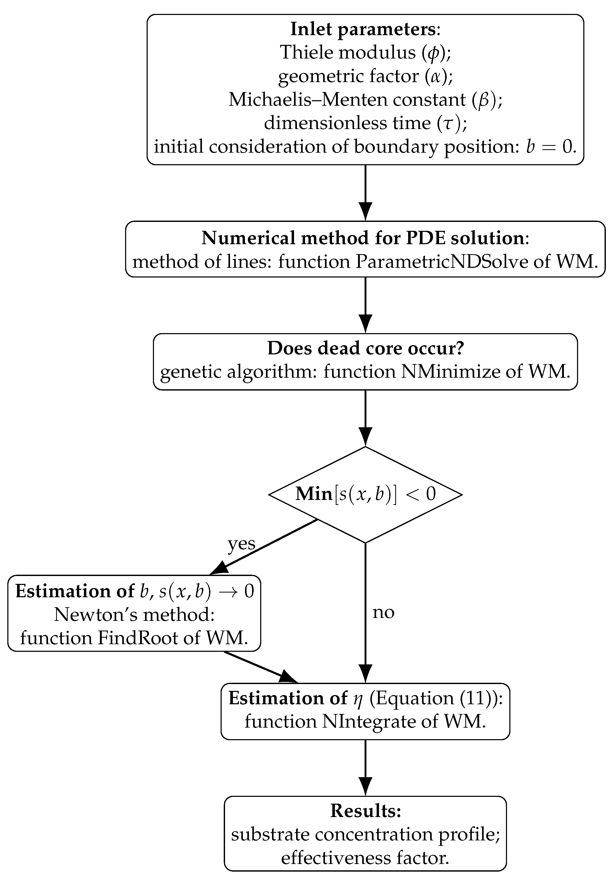
Figure 2 presents the flowchart of the numerical procedure used to compute (i) the concentration profile inside the particle, (ii) the catalytic effectiveness factor, and (iii) the position of the moving boundary associated with a possible dead core.

As depicted in Figure 2, the PDE is solved first to obtain the substrate concentration profile. Next, the solution is checked to determine whether any region within the particle is completely depleted of substrate (dead core), which is assessed by identifying the minimum concentration in the domain. If the concentration remains non-negative throughout the particle, the calculation of the effectiveness factor $\eta$ (Equation (20)) follows directly. If a negative value is detected, the presence of a dead core is indicated, and the internal boundary position is subsequently re-estimated.

Finally, note that the internal boundary is estimated with Newton’s method (function FindRoot of WM) only at the final simulation time $\tau$. Because the particle starts fully depleted and substrate diffuses inwards over time, ensuring a physically meaningful (non-negative) profile is most restrictive at the final time. Therefore, it is unnecessary to embed Newton updates inside each intermediate time step of the method-of-lines solver, which keeps the numerical procedure simpler and more robust. As an additional consistency check, this choice is validated for a large value of $\tau$ (practically steady state) by comparing the numerically estimated effectiveness factor ($\eta$) with the corresponding analytical steady-state expressions for the zero-order and first-order kinetics (Equations (24) and (28)–(30)). The agreement confirms the correctness of the proposed procedure.

2.5. Simulation of a Continuous Stirred Tank Reactor (CSTR) Using Literature-Based Parameters

The practical application of the MLN is illustrated through the simulation of a CSTR performing the enzymatic hydrolysis of sucrose using cell-based invertase immobilized in calcium alginate, a chemically relevant and widely studied catalytic system. Kinetic parameters and operating conditions were adopted from the literature [48,49].

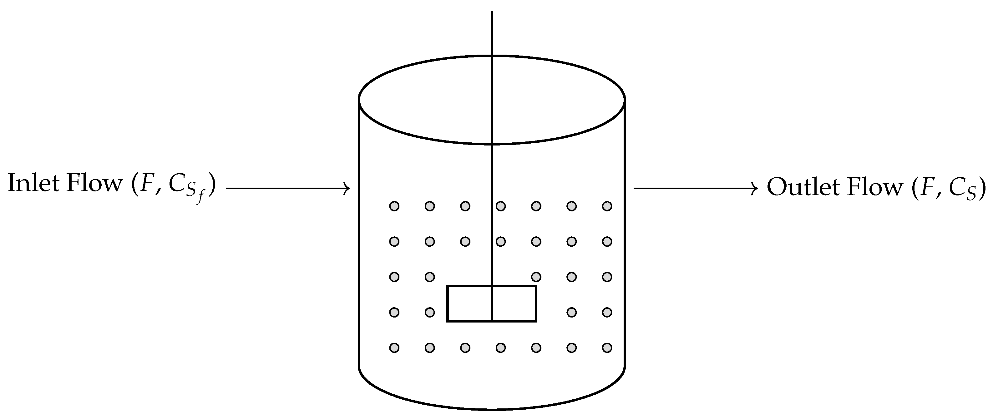
Figure 3 shows a schematic representation of the CSTR simulated in this study.

The substrate mass balance in the CSTR is given by Equation (31), where $C_{S_f}$ is the concentration of substrate in the feed, F is the volumetric flow rate, $V_L$ is the working volume of the reactor, $\gamma$ represents the effective catalyst loading per unit reactor volume (factor required to convert the intrinsic reaction rate defined per unit mass of biocatalyst into a volumetric reaction rate based on $V_L$).

$${\displaystyle \frac{d{C}_S}{dt}}={\displaystyle \frac{F}{V_L}}(C_{S_f}-C_S)-\gamma ·\eta ·v_{max}·{\displaystyle \frac{C_S}{K_M+C_S}}$$

(31)

The initial condition to solve Equation (31) is $C_S=C_{S_f}$ at $t=0$, which represents a reactor initially charged with feed medium.

The simulations were performed using the operating conditions, kinetic parameters and diffusion coefficient given in

Table 1. Operating conditions and kinetic/transport parameters used in the CSTR simulation [48,49].

Condition/Parameter	Value	Units
F	$0.001$	L/min
$C_{S_f}$	10	g/L
$V_L$	$0.01$	L
$\gamma$	15	Dimensionless
$v_{max}$	0.085	g/(L·min)
$K_M$	$19.0$	g/L
$D_{ef}$	$4.1\times {10}^{-6}$	cm2/s

[48,49].

This simulation was performed to evaluate the accuracy and practical implications of the proposed method; two different approaches for calculating the effectiveness factor were compared in the simulation of substrate consumption by immobilized enzymes. The method developed in this study explicitly accounts for the transient intraparticle concentration profile, yielding a time-dependent effectiveness factor that captures the dynamic evolution of mass transfer and reaction within the catalytic particle. In contrast, the conventional approach widely adopted in the literature assumes an instantaneous attainment of the intraparticle steady state, calculating a steady-state effectiveness factor at each time step of the reactor simulation [50]. While this approximation simplifies the mathematical treatment, it neglects the transient diffusion–reaction phenomenon that is particularly relevant during non-steady operating conditions.

3. Results and Discussion

The proposed method was applied to solve problems involving catalytic particles with classical geometries (planar, cylindrical, and spherical) under the following conditions: (i) Thiele modulus ($\varphi$) ranging from 0.01 to 100; (ii) dimensionless MM constant ($\beta$) varying from zero (zero-order kinetics) to ∞ (first-order kinetics); and (iii) dimensionless time ($\tau$) from zero to 10. For all cases analyzed, the numerical method provided phenomenologically consistent solutions.

3.1. Transient Profiles of Substrate Concentration Intraparticle

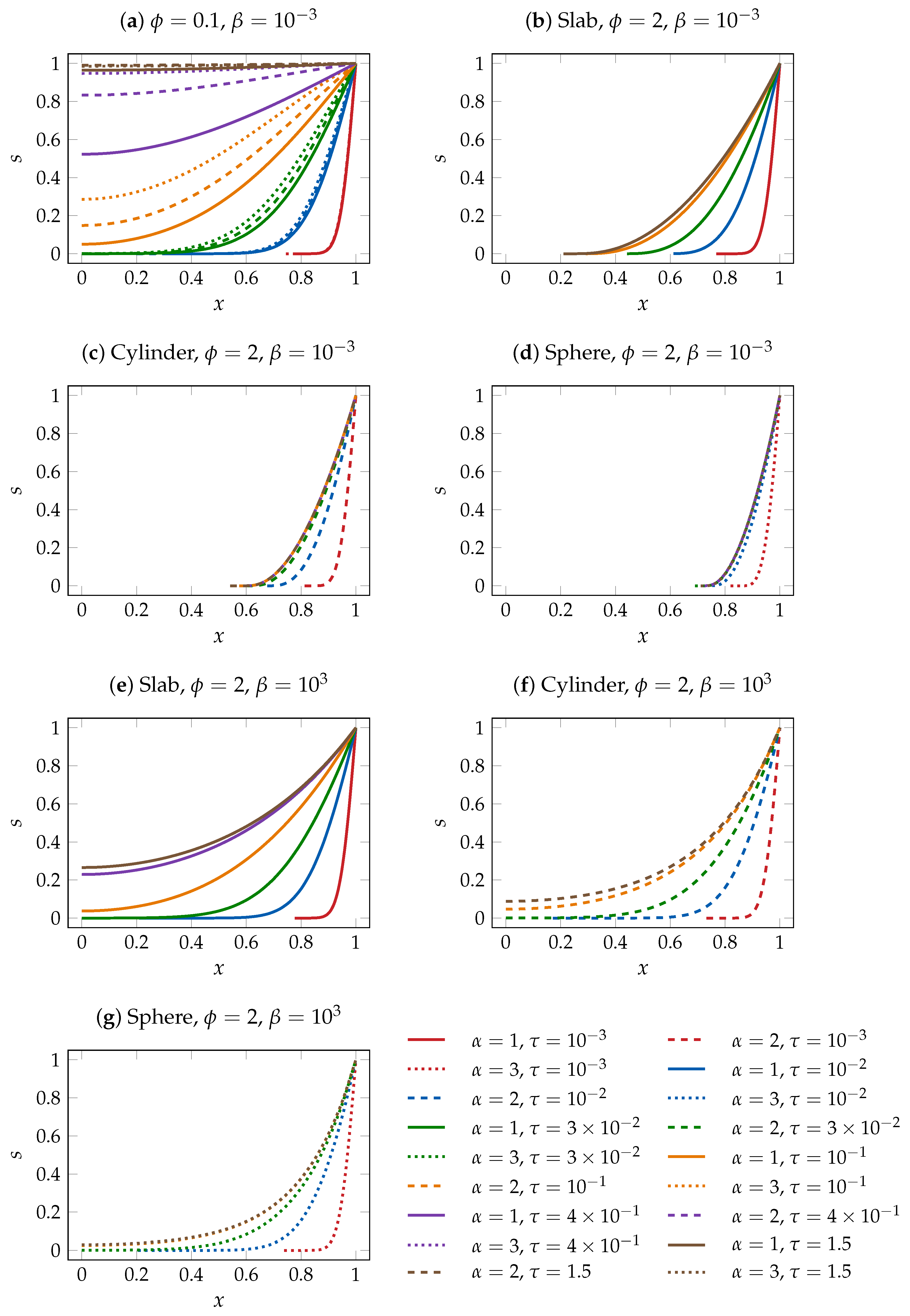
Typical transient profiles of substrate concentration within the particle were obtained, as shown in Figure 4, where the dimensionless time ranged from $\tau =0$ (initial contact between the immobilized enzyme particle and the reaction medium containing substrate) to $\tau =10$. This value was assumed as the practical steady-state criterion, since the concentration profiles approach a quasi-steady state around $\tau \approx 3$ and remain essentially constant thereafter.

Figure 4a–d compare the transient concentration profiles for different values of the Thiele modulus ($\varphi$) at a low value of the dimensionless MM constant ($\beta ={10}^{-3}$). For low $\varphi$ (Figure 4a), a transient dead-core shrinkage is observed only at very small $\tau$ values. In this case, the substrate easily penetrates the inner regions of the particle, reaching concentrations close to those at the surface throughout the catalyst, which is consistent with the physical phenomenon since low $\varphi$ values correspond to a smaller ratio between reaction rate and diffusion rate.

For higher $\varphi$ values and low $\beta$ values (Figure 4b–d), the dead core shrinks as $\tau$ increases, and a permanent dead core may occur at steady state. To illustrate this phenomenon, the $\varphi$ and $\beta$ values in Figure 4a–d were intentionally chosen because for low $\beta$, the MM kinetics approaches zero-order behavior. In this case, the critical $\varphi$ values (above which a permanent dead core is observed at steady state) are $\sqrt{2}$ for slab particles, one for cylindrical particles, and $\sqrt{6}/3$ for spherical particles.

All curves described in the legend of Figure 4 were plotted in Figure 4a–g. Curves not visible in the figures are overlapped at steady state. Considering this overlap and focusing on Figure 4b–d (high $\varphi$ values and low $\beta$ values, where a permanent dead core may occur), steady state is reached faster for spherical particles, followed by cylindrical, and finally slab particles. This trend is explained by the size of the permanent dead core: larger for spheres (lower critical $\varphi$), intermediate for cylinders, and smaller for slabs (higher critical $\varphi$).

The effect of the $\beta$ parameter becomes evident when comparing Figure 4b–d ($\beta ={10}^{-3}$) with Figure 4e–g ($\beta ={10}^3$): a low $\beta$, associated with pseudo–zero-order kinetics, renders the reaction rate independent of the substrate concentration, so that the solution of the diffusion–reaction problem may reach zero substrate concentration within the particle, leading to the establishment of a permanent dead core; in contrast, a high $\beta$, corresponding to pseudo–first-order kinetics, causes the reaction rate to decrease linearly with the substrate concentration, thereby avoiding the establishment of a permanent dead core.

Several simulations were performed for different values of $\varphi$, $\beta$, and $\tau$, consistently yielding behaviors in agreement with the expected reaction–diffusion phenomenon under transient conditions, within the limitations imposed by the assumptions (isothermal system and negligible external diffusion resistance). The proposed methodology produced smooth and physically consistent concentration profiles without numerical noise. Based on these reliable profiles, it was possible to proceed with the analysis of the dynamic behavior of the effectiveness factor and, subsequently, to compare the effectiveness factor values obtained in this study with those reported in previous works using the method of orthogonal collocation on finite elements and with analytical solutions for zero- and first-order kinetics at steady state.

3.2. Transient Effectiveness Factor

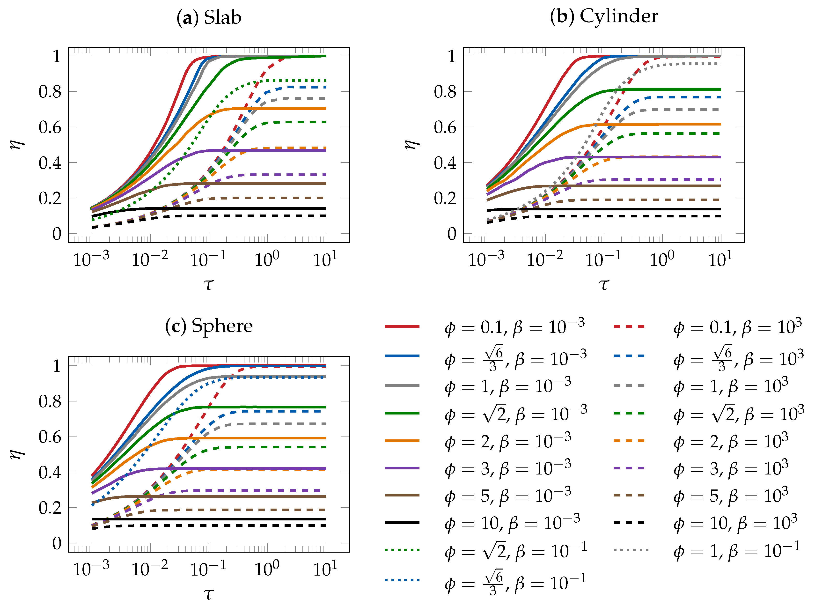
In general, the transient behavior of the effectiveness factor exhibited the trend shown in Figure 5. In Figure 5a–c, the Thiele modulus was selected based on its critical values ($\sqrt{2}$ for slabs, 1 for cylinders, and $\sqrt{6}/3$ for spheres), as well as values below and above these thresholds, in order to generate distinct curves. Additionally, three values of the dimensionless MM constant were considered: $\beta ={10}^{-3}$ (approaching zero-order kinetics, solid lines), $\beta ={10}^3$ (approaching first-order kinetics, dashed lines), and $\beta ={10}^{-1}$ (intermediate behavior, dotted lines).

According to Figure 5a–c, the rate of change of $\eta$ with respect to $\tau$ (i.e., d$\eta$/d$\tau$) is greater for smaller values of $\varphi$, since under these conditions the substrate diffusion rates are higher than those for larger $\varphi$ values. Consequently, the time required for the effectiveness factor to reach steady state depends on both the diffusion rate and the difference, in terms of substrate concentration, between the initial condition (always zero) and the steady-state value.

Figure 5a–c show a clear trend: the effectiveness factor increases as $\beta$ decreases (for the same $\varphi$ and $\tau$). This behavior reflects the shift in the apparent order of the MM kinetics as $\beta$ varies. Lower $\beta$ values (e.g., ${10}^{-3}$) correspond to conditions approaching zero-order kinetics, where the reaction rate is less dependent on substrate concentration and less affected by internal diffusional limitations. Conversely, higher $\beta$ values (e.g., ${10}^3$) approach first-order kinetics, making the reaction rate strongly dependent on substrate concentration and more influenced by intraparticle diffusion resistance.

Considering that the observed behavior of the effectiveness factor is consistent with the expected reaction–diffusion mechanism described in this study, with smooth profiles and absence of numerical noise, and given that analytical solutions exist for the limiting cases where MM kinetics approaches the zeroth order (low $\beta$ values) and first order (high $\beta$ values) at steady state, it was possible to assess the proposed method in terms of its ability to provide reliable effectiveness factor values.

Physical Interpretation: Pore Structure, Transport Pathways, and Dead-Core Dynamics

A mechanistic viewpoint of dead-core dynamics and of the transient evolution of the effectiveness factor emerges when the dimensionless parameters are interpreted in terms of pore-scale transport. The Thiele modulus $\varphi$ measures the capacity of a reaction to deplete substrate relative to the capacity of diffusion to replenish it; microscopically, a large $\varphi$ is consistent with narrower or more tortuous pores, reduced effective diffusivity, or higher enzyme loading along pore walls, all of which limit penetration depth and favor a depleted inner region [8,45]. In our results, this manifests as a thicker reacting shell and persistent dead core for the high-$\varphi$ cases in Figure 4b–d ($\varphi =2$, $\beta ={10}^{-3}$), with a slower approach of $\eta$ to its plateau in Figure 5, when diffusion limits substrate replenishment.

The parameter $\beta$ links directly to the order from the simplified MM kinetics: at low $\beta$ values the kinetics behaves closer to the zeroth order (enzyme saturated), sustaining a reaction rate along deeper pores and sharpening the transition between active and depleted regions. For high $\beta$ values the MM kinetics approaches the first-order kinetics (unsaturated), reducing the reaction rate in low-substrate-concentration zones and enabling deeper penetration with smoother gradients [44,45]. This shift is visible when comparing Figure 4b–d ($\beta ={10}^{-3}$) with Figure 4e–g ($\beta ={10}^3$). Figure 4e–g ($\beta ={10}^3$) do not show a permanent dead core and exhibit smooth profiles, a behavior that also explains the faster rise of $\eta$ for high $\beta$ values in Figure 5 (dashed lines).

Geometric factors further modulate the intraparticle substrate concentration profiles by altering the local balance between diffusive supply and internal consumption: slab, cylindrical, and spherical particles exhibit progressively different diffusion path lengths and surface-to-volume ratios, which directly shape substrate penetration and depletion patterns [8]. Consistent with this phenomenological interpretation, Figure 4 shows that spherical particles, due to shorter diffusion path lengths and more favorable surface-to-volume ratios, develop intraparticle substrate concentration profiles with faster inward penetration, leading to a more pronounced and earlier decline of the substrate concentration profile (for the same values of $(\varphi ,\beta )$) and to a faster approach to a quasi-steady regime of $\eta \left(\tau \right)$ in Figure 5, whereas slab-type geometries sustain broader regions of substrate depletion and longer transients as a direct consequence of their less favorable diffusion pathways. Critical behaviors reported for limiting kinetics (e.g., zero-order thresholds for dead-core formation) are also consistent with classical analyses of catalytic pellets.

Taken together, the phenomenological trends previously discussed establish a direct link between the diffusion–reaction parameters $(\varphi ,\beta )$, the geometry index $\alpha$, and physical characteristics of the catalytic material, such as pore size, tortuosity, accessible diffusion pathways, and the saturation degree of active sites thereby providing a consistent physical explanation for the dead-core shrinkage observed in Figure 4 and for the corresponding trajectories of $\eta$ in Figure 5.

3.3. Steady-State Approximation (SSA)

The transient behavior of the effectiveness factor shown in Figure 5 indicates that steady state is fully reached for $\tau$ values greater than three. To ensure this condition, a value of $\tau =10$ was adopted for evaluating the steady-state approximation (SSA) errors generated by the proposed numerical method. The effectiveness factor values calculated under the steady-state assumption (${\eta }_{ss}$) were then compared with the corresponding analytical solutions (${\eta }_a$) derived from the simplified MM kinetics for zero- and first-order cases. Additionally, the values of $\eta$ obtained using the method of orthogonal collocation on finite elements (${\eta }_{oc}$) [18] were also compared with the analytical values (${\eta }_a$) to assess the accuracy of the proposed method relative to a previously developed approach.

Table 2. Comparison between steady-state approximation and the method of orthogonal collocation on finite elements.

Order	$\mathit{\alpha }$	$\mathit{\varphi }$	b	$\mathit{\eta }$	${\mathit{\epsilon }}_{\mathbf{oc}}$	${\mathit{\epsilon }}_{\mathbf{ss}}$
0	1	0.5	0	1	$5.7\times {10}^{-11}$	$8.9\times {10}^{-16}$
0	1	1	0	1	$1.1\times {10}^{-11}$	$8.9\times {10}^{-16}$
0	1	2	0.2929	0.7071	$2.6\times {10}^{-11}$	$4.4\times {10}^{-11}$
0	1	4	0.6464	0.3536	$2.7\times {10}^{-11}$	$6.3\times {10}^{-11}$
0	1	8	0.8232	0.1768	$2.8\times {10}^{-11}$	$3.0\times {10}^{-10}$
0	2	0.5	0	1	$9.0\times {10}^{-12}$	$8.9\times {10}^{-16}$
0	2	1	0	1	$2.0\times {10}^{-12}$	$1.1\times {10}^{-15}$
0	2	2	0.6184	0.6176	$3.6\times {10}^{-11}$	$1.1\times {10}^{-8}$
0	2	4	0.8173	0.332	$3.3\times {10}^{-11}$	$7.9\times {10}^{-10}$
0	2	8	0.9102	0.1715	$3.8\times {10}^{-11}$	$2.1\times {10}^{-10}$
0	3	0.5	0	1	$2.9\times {10}^{-12}$	$1.1\times {10}^{-15}$
0	3	1	0.3869	0.9421	$8.8\times {10}^{-14}$	$8.6\times {10}^{-8}$
0	3	2	0.7402	0.5934	$1.1\times {10}^{-12}$	$3.2\times {10}^{-8}$
0	3	4	0.8769	0.3255	$7.7\times {10}^{-12}$	$2.8\times {10}^{-10}$
0	3	8	0.9398	0.1698	$3.0\times {10}^{-11}$	$2.8\times {10}^{-10}$
1	1	0.5	0	0.9242	$5.1\times {10}^{-11}$	$2.2\times {10}^{-10}$
1	1	1	0	0.7616	$8.4\times {10}^{-12}$	$2.4\times {10}^{-10}$
1	1	2	0	0.482	$8.5\times {10}^{-13}$	$3.7\times {10}^{-10}$
1	1	4	0	0.2498	$7.6\times {10}^{-14}$	$3.1\times {10}^{-9}$
1	1	8	0	0.125	$1.1\times {10}^{-12}$	$2.5\times {10}^{-8}$
1	2	0.5	0	0.8928	$7.0\times {10}^{-12}$	$2.6\times {10}^{-12}$
1	2	1	0	0.6978	$1.1\times {10}^{-12}$	$1.3\times {10}^{-10}$
1	2	2	0	0.4318	$1.2\times {10}^{-13}$	$2.6\times {10}^{-9}$
1	2	4	0	0.2338	$2.1\times {10}^{-12}$	$3.1\times {10}^{-8}$
1	2	8	0	0.121	$8.5\times {10}^{-10}$	$2.2\times {10}^{-7}$
1	3	0.5	0	0.8762	$2.0\times {10}^{-12}$	$1.1\times {10}^{-11}$
1	3	1	0	0.6716	$2.3\times {10}^{-13}$	$4.1\times {10}^{-10}$
1	3	2	0	0.4167	$2.4\times {10}^{-13}$	$9.3\times {10}^{-9}$
1	3	4	0	0.2292	$1.0\times {10}^{-10}$	$1.1\times {10}^{-7}$
1	3	8	0	0.1198	$3.3\times {10}^{-8}$	$4.7\times {10}^{-7}$

presents the errors in the effectiveness factor calculated by the SSA (${\epsilon }_{ss}=|{\eta }_{ss}-{\eta }_a|$) and by the method of orthogonal collocation on finite elements (${\epsilon }_{oc}=|{\eta }_{oc}-{\eta }_a|$).

The data in Table 2 demonstrate that the SSA method proposed in this study provides highly accurate solutions to the reaction–diffusion problem in biocatalytic particles. Compared to the method of orthogonal collocation on finite elements, the main advantages of the proposed approach are its ease of implementation in WM software and the absence of any requirement for an initial estimate of the substrate concentration profile within the particle.

3.4. Sensitivity and Numerical Uncertainty

The sensitivity and numerical robustness of the MLN during transient regime were assessed by combining information from Figure 4 and Figure 5 and Table 2.

In agreement with the trends shown in Figure 4 and Figure 5, the sensitivity of $\eta$ to the Thiele modulus ($\varphi$) is pronounced in diffusion-limited conditions ($\varphi \gtrsim 1$) and weak in reaction-limited conditions ($\varphi \lesssim 0.1$). The dependence on $\beta$ parameter reflects the expected shift in the order of the apparent kinetic: zero-order kinetics, for lower $\beta$ values, favors the formation of a permanent dead core, particularly at higher values of $\varphi$, while for high $\beta$ values, first-order kinetics prevents the occurrence of a permanent dead core, leading to smoother concentration profiles and milder changes in $\eta$.

To evaluate the numerical uncertainty of the MLN method in calculating a zero substrate concentration at the moving-boundary position $x=b$,

Table 3. Numerical uncertainty associated with the MLN method in obtaining a zero substrate concentration at the moving-boundary position for $\varphi =2$ and $\beta ={10}^{-3}$.

Geometry	$\mathit{\tau }$	b	${\mathit{s}}_{\mathit{x}=\mathit{b}}$
slab	${10}^{-3}$	0.8	$5\times {10}^{-9}$
Slab	${10}^{-2}$	0.6	$7\times {10}^{-4}$
Slab	$3\times {10}^{-2}$	0.4	$1\times {10}^{-4}$
Slab	${10}^{-1}$	0.3	$1\times {10}^{-4}$
Slab	$4\times {10}^{-1}$	0.2	$7\times {10}^{-12}$
Slab	$1.5$	0.2	$1\times {10}^{-11}$
Cylinder	${10}^{-3}$	0.8	$2\times {10}^{-6}$
Cylinder	${10}^{-2}$	0.7	$4\times {10}^{-5}$
Cylinder	$3\times {10}^{-2}$	0.6	$8\times {10}^{-5}$
Cylinder	${10}^{-1}$	0.6	$3\times {10}^{-11}$
Cylinder	$4\times {10}^{-1}$	0.6	$1\times {10}^{-4}$
Cylinder	$1.5$	0.5	$7\times {10}^{-16}$
Sphere	${10}^{-3}$	0.8	$4\times {10}^{-7}$
Sphere	${10}^{-2}$	0.8	$6\times {10}^{-4}$
Sphere	$3\times {10}^{-2}$	0.7	$2\times {10}^{-12}$
Sphere	${10}^{-1}$	0.7	$1\times {10}^{-4}$
Sphere	$4\times {10}^{-1}$	0.7	$1\times {10}^{-4}$
Sphere	$1.5$	0.7	$3\times {10}^{-10}$

presents, for each curve shown in Figure 4b–d, which ones display dead-core shrinkage data for $\varphi =2$ and $\beta ={10}^{-3}$.

Overall, the data presented in Table 3 support both the numerical robustness and the physical consistency of the MLN in tracking dead-core shrinkage. The substrate concentration at the boundary $x=b$ is close to zero for all geometries during the transient period, confirming that the moving-boundary condition is satisfied. The substrate concentrations calculated at the moving-boundary position ($x=b$) range between $7\times {10}^{-16}$ and $1\times {10}^{-4}$ for all cases reported in Table 3. These values can be regarded as practically zero. From a physical viewpoint, these numerical uncertainties do not affect the determination of either b or $\eta$.

3.5. Simulation of CSTR

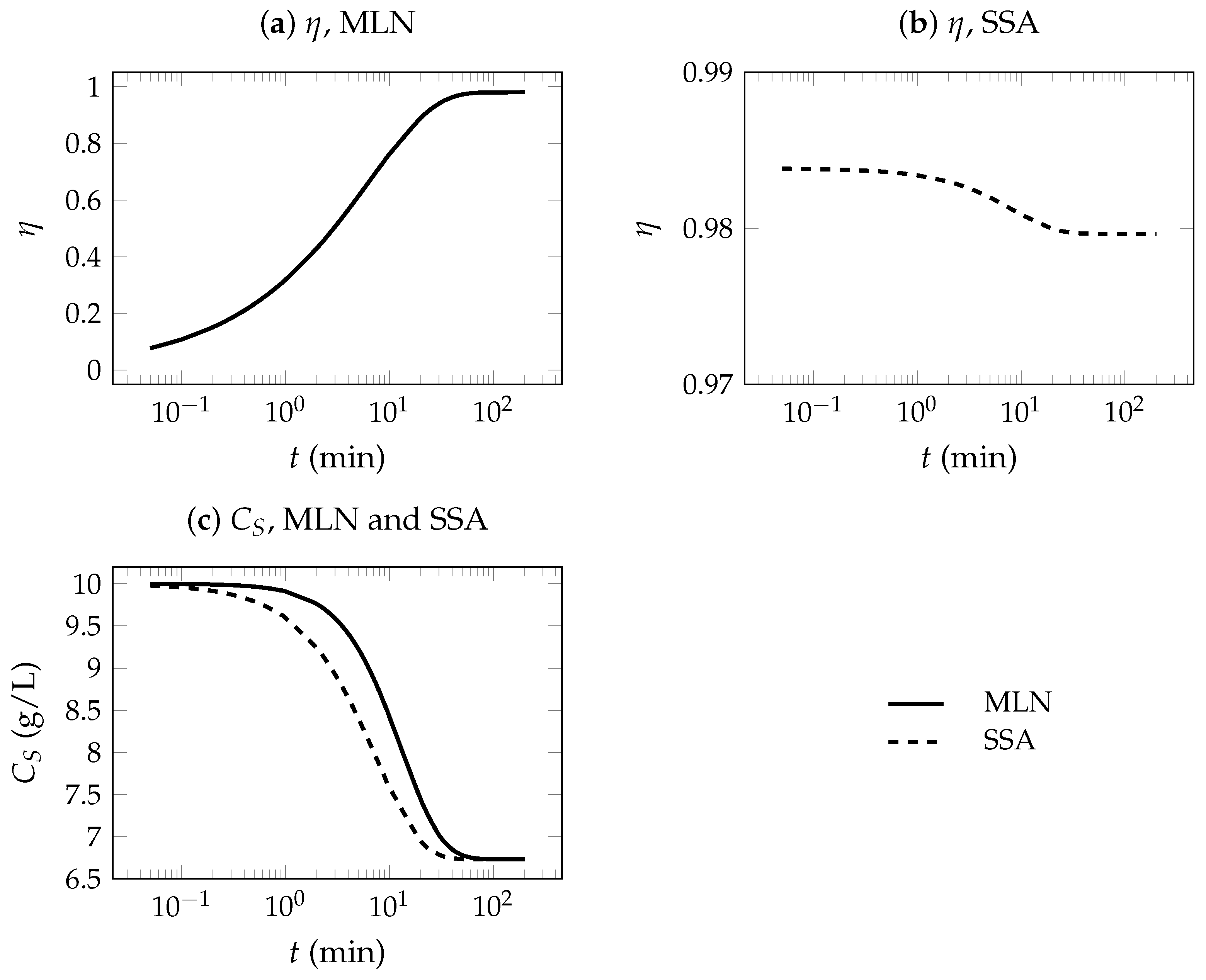
Figure 6 shows the CSTR simulation results for sucrose hydrolysis catalyzed by invertase, including the transient effectiveness factor and substrate concentration profiles obtained with the MLN and SSA methods.

In the MLN-based approach, (Figure 6a), the effectiveness factor ($\eta$) starts at low values because during reactor startup, there is no substrate inside the particles (a). As the substrate concentration increases due to diffusion, the effectiveness factor rises, reflecting the progressive activation of the catalytic sites within the particles.

In the SSA method, the intraparticle concentration profile is assumed to be the steady-state profile corresponding to the bulk substrate concentration. As a consequence, the effectiveness factor $\eta$ is overestimated during reactor startup (Figure 6b), leading to higher predicted reaction rates and a faster decrease in substrate concentration in comparison to those of the MLN (Figure 6c).

Overall, the results highlight that considering a realistic initial substrate concentration profile is essential to accurately describe the CSTR startup behavior, as provided by the MLN approach.

4. Conclusions

Heterogeneous reactors with immobilized enzymes are industrially important for the synthesis of numerous bioproducts, offering the advantage of reusing the biocatalyst multiple times. However, immobilizing enzymes on solid supports introduces a problem: resistance to substrate diffusion within the catalytic particle toward the enzyme’s active sites.

Initially, when the particle is exposed to the substrate, its interior is catalytically inactive (dead core) because the substrate is absent. Over time, the substrate diffuses into the particle, accumulates, and reacts, leading to the shrinkage of the initial dead core. This diffusion–reaction process continues, generating successive temporal profiles of substrate concentration until a steady state is reached, in which two distinct situations may occur: the formation of a permanent dead core or its complete disappearance.

These diffusional effects on the reaction rate can be quantified by the catalytic effectiveness factor ($\eta$), a parameter ranging between zero and one. A value of zero represents a completely inactive particle with zero average reaction rate, while a value of one corresponds to a fully active particle, free from internal diffusional limitations, with an average reaction rate equal to that at the particle surface.

The effectiveness factor is a key parameter in the design of heterogeneous reactors, and its determination requires solving the space–time equation representing the diffusion–reaction problem with a moving-boundary condition. Depending on the reaction kinetics, this equation has been solved analytically or numerically by several methods, including the method of orthogonal collocation on finite elements (more laborious) and the simpler method proposed in this study.

The simulated results demonstrated that the proposed method provided accurate solutions to the steady-state reaction–diffusion problem when compared with analytical solutions for the limiting cases of zero-order and first-order MM kinetics.

From an engineering perspective, these findings highlight that the choice of numerical approach should be guided by operational characteristics. While SSA approach may be adequate for long-term operation far from startup, the MLN approach becomes necessary whenever transient behavior is relevant, such as during reactor startup, shutdown, or other non-stationary operations. Therefore, the numerical methodology developed in this study provides a valuable and practical tool to support the design, operation, and scale-up of heterogeneous biocatalytic reactors under realistic operating conditions.

References

1. Jothyswarupha, K.; Venkataraman, S.; Rajendran, D.S.; Shri, S.S.; Sivaprakasam, S.; Yamini, T.; Karthik, P.; Kumar, V.V. Immobilized enzymes: Exploring its potential in food industry applications. Food Sci. Biotechnol. 2025, 34, 1533–1555. [Google Scholar] [CrossRef] [PubMed]
2. Farhan, M.; Hasani, I.W.; Khafaga, D.S.; Ragab, W.M.; Ahmed Kazi, R.N.; Aatif, M.; Muteeb, G.; Fahim, Y.A. Enzymes as catalysts in industrial biocatalysis: Advances in engineering, applications, and sustainable integration. Catalysts 2025, 15, 891. [Google Scholar] [CrossRef]
3. Tavares, B.; Felipe, M.d.G.d.A.; Santos, J.C.; Pereira, F.M.; Gomes, S.D.; Sene, L. An experimental and modeling approach for ethanol production by Kluyveromyces marxianus in stirred tank bioreactor using vacuum extraction as a strategy to overcome product inhibition. Renew. Energy 2019, 131, 261–267. [Google Scholar] [CrossRef]
4. Pereira, F.M.; Loures, C.C.; Amaral, M.S.; Gomes, F.M.; Pedro, G.A.; Machado, M.A.; Reis, C.E.; Silva, M.B. Evaluation of fatty acids production by Chlorella minutissima in batch bubble-column photobioreactor. Fuel 2018, 230, 155–162. [Google Scholar] [CrossRef]
5. Ferreira-Leitão, V.; Cammarota, M.; Gonçalves Aguieiras, E.; Vasconcelos de Sá, L.; Fernandez-Lafuente, R.; Freire, D. The protagonism of biocatalysis in green chemistry and its environmental benefits. Catalysts 2017, 7, 9. [Google Scholar] [CrossRef]
6. Prado, C.; Raymundo, M.; Shibukawa, V.; Jofre, F.; Cruz-Santos, M.M.; Arruda, G.; dos Santos, D.; Silos, N.; Reis, W.; da Silva, S.; et al. Bioreactors Configuration in the Development of Process Consolidation for Biofuels and Biochemicals in Lignocellulosic Biorefineries. In Biorefineries in Circular Bioeconomy: Reactor Configurations Analysis; Springer: Berlin/Heidelberg, Germany, 2026; pp. 187–210. [Google Scholar]
7. Illanes, A. Enzyme Biocatalysis; Springer: Berlin/Heidelberg, Germany, 2008. [Google Scholar]
8. Fogler, H.S. Essentials of Chemical Reaction Engineering; Pearson Education: London, UK, 2010. [Google Scholar]
9. Mahunu, G.K.; Mildred, O.K.; Peter, S. Biotechnology of microbial enzymes. In Microbial Enzymes; Elsevier: Amsterdam, The Netherlands, 2026; pp. 173–184. [Google Scholar]
10. Cocco, G.; Cocco, A.; Sollai, F.; Sanjust, E.; Zucca, P. Bioinspired versus Enzymatic Oxidation of Some Homologous Thionine Dyes in the Presence of Immobilized Metalloporphyrin Catalysts and Ligninolytic Enzymes. Int. J. Mol. Sci. 2017, 18, 2553. [Google Scholar] [CrossRef]
11. Liese, A.; Hilterhaus, L. Evaluation of immobilized enzymes for industrial applications. Chem. Soc. Rev. 2013, 42, 6236–6249. [Google Scholar] [CrossRef]
12. Sharma, A.; Singh, A.; Sidhu, S.; Arya, S.K.; Singh, G. Insights on the recent trends and advancements in enzyme immobilization strategies. In Recent Trends in Enzyme Immobilization; Elsevier: Amsterdam, The Netherlands, 2026; pp. 165–186. [Google Scholar]
13. Rumpke, K.; Killi, N.; Dittrich, B.; Herrmann, A.; Kuckling, D. Nanofiber Mats as Amine-Functionalized Heterogeneous Catalysts in Continuous Microfluidic Reactor Systems. Gels 2026, 12, 55. [Google Scholar] [CrossRef]
14. Ye, T.H.; Hanh, N.T.D.; Gao, Y.H.; Seubsai, A.; Hansupalak, N.; Imyen, T.; Chiu, C.Y.; Chen, K.H.; Liu, B.L.; Chang, Y.K. Modular nanofiber membrane reactor with site-selective carbonic anhydrase immobilization on regenerated cellulose for enhanced CO2 conversion and mineralization. Sep. Purif. Technol. 2026, 388, 136738. [Google Scholar] [CrossRef]
15. Elakkya, M.; Swaminathan, R. Mathematical modelling of the Phenol-Polyphenol Oxidase system for amperometric immobilized enzymes at spherical electrode. Partial Differ. Equ. Appl. Math. 2025, 14, 101140. [Google Scholar] [CrossRef]
16. Selvi, M.S.M.; Hariharan, G.; Kannan, K. A Reliable Spectral Method to Reaction–Diffusion Equations in Entrapped-Cell Photobioreactor Packed with Gel Granules Using Chebyshev Wavelets. J. Membr. Biol. 2017, 250, 663–670. [Google Scholar] [CrossRef] [PubMed]
17. Król, G.; Szukiewicz, M.; Chutkowski, M. Formation of dead zone in catalytic particles in catalysis and biocatalysis—New alternative method of determination. Can. J. Chem. Eng. 2018, 97, 1525–1536. [Google Scholar] [CrossRef]
18. Pereira, F.M.; Oliveira, S.C. Occurrence of dead core in catalytic particles containing immobilized enzymes: Analysis for the Michaelis–Menten kinetics and assessment of numerical methods. Bioprocess Biosyst. Eng. 2016, 39, 1717–1727. [Google Scholar] [CrossRef] [PubMed][Green Version]
19. Petkevičius, L.; Baronas, R. Numerical simulation and analysis of enzyme-catalysed substrate conversion in a microbioreactor. Int. J. Adv. Syst. Meas. 2018, 11, 173–182. [Google Scholar]
20. Rajaraman, R. Exploring Nonlinear Reaction–Diffusion in Enzyme Immobilized Systems: Integer and Fractional Order Modeling. Appl. Biochem. Biotechnol. 2025, 197, 793–820. [Google Scholar] [CrossRef]
21. Noorman, S.; Gallucci, F.; van Sint Annaland, M.; Kuipers, J. A theoretical investigation of CLC in packed beds. Part 1: Particle model. Chem. Eng. J. 2011, 167, 297–307. [Google Scholar] [CrossRef]
22. Noorman, S.; Gallucci, F.; van Sint Annaland, M.; Kuipers, J. A theoretical investigation of CLC in packed beds. Part 2: Reactor model. Chem. Eng. J. 2011, 167, 369–376. [Google Scholar] [CrossRef]
23. Abdul Wasay, S.; Shen, J.; Salmon, S.; Bolotnov, I. Modeling CO2 Mass Transfer Dynamics in Falling Liquid Films Over Textile Fiber Surfaces. In Proceedings of the 2025 Biocatalyst Interactions with Gases (BIG) Research Symposium, Raleigh, NC, USA, 14–16 May 2025. [Google Scholar]
24. Oltean, M.; Sopuerta, C.F.; Spallicci, A.D. Particle-without-Particle: A practical pseudospectral collocation method for linear partial differential equations with distributional sources. J. Sci. Comput. 2019, 79, 827–866. [Google Scholar] [CrossRef]
25. Strouwen, A.; Nicolaï, B.M.; Goos, P. Optimizing Oxygen Input Profiles for Efficient Estimation of Michaelis-Menten Respiration Models. Food Bioprocess Technol. 2019, 12, 769–780. [Google Scholar] [CrossRef]
26. Feng, S.; Zhou, L.; Zhang, Y.; Lü, S.; Long, M. Mechanochemical modeling of neutrophil migration based on four signaling layers, integrin dynamics, and substrate stiffness. Biomech. Model. Mechanobiol. 2018, 17, 1611–1630. [Google Scholar] [CrossRef]
27. Abbas, M.; Majid, A.A.; Ismail, A.I.M.; Rashid, A. Numerical method using cubic B-spline for a strongly coupled reaction-diffusion system. PLoS ONE 2014, 9, e83265. [Google Scholar] [CrossRef] [PubMed]
28. He, J.H. Some asymptotic methods for strongly nonlinear equations. Int. J. Mod. Phys. B 2006, 20, 1141–1199. [Google Scholar] [CrossRef]
29. PonRani, V.M.; Rajendran, L. Mathematical modelling of steady-state concentration in immobilized glucose isomerase of packed-bed reactors. J. Math. Chem. 2012, 50, 1333–1346. [Google Scholar] [CrossRef]
30. Saranya, J.; Rajendran, L.; Wang, L.; Fernandez, C. A new mathematical modelling using Homotopyperturbation method to solve nonlinear equations in enzymatic glucose fuel cells. Chem. Phys. Lett. 2016, 662, 317–326. [Google Scholar] [CrossRef]
31. Selvi, M.S.M.; Hariharan, G.; Kannan, K.; Heydari, M. Two reliable computational methods pertaining to steady state substrate concentration of an immobilized enzyme system. Alex. Eng. J. 2017, 57, 2377–2385. [Google Scholar] [CrossRef]
32. Selvi, M.S.M.; Hariharan, G. Wavelet-based analytical algorithm for solving steady-state concentration in immobilized glucose isomerase of packed-bed reactor model. J. Membr. Biol. 2016, 249, 559–568. [Google Scholar] [CrossRef]
33. Tian, X.; Liao, Q.; Liu, W.; Wang, Y.Z.; Zhu, X.; Li, J.; Wang, H. Photo-hydrogen production rate of a PVA-boric acid gel granule containing immobilized photosynthetic bacteria cells. Int. J. Hydrogen Energy 2009, 34, 4708–4717. [Google Scholar] [CrossRef]
34. Gupta, A.; Ray, S.S. Numerical treatment for the solution of fractional fifth-order Sawada–Kotera equation using second kind Chebyshev wavelet method. Appl. Math. Model. 2015, 39, 5121–5130. [Google Scholar] [CrossRef]
35. Guo, F.; Zhuang, D. Real-time monitoring and prediction of glucose content in enzymatic reactions: Application of a deep neural network mode. Food Biosci. 2025, 64, 105804. [Google Scholar] [CrossRef]
36. Pakdaman, M.; Ahmadian, A.; Effati, S.; Salahshour, S.; Baleanu, D. Solving differential equations of fractional order using an optimization technique based on training artificial neural network. Appl. Math. Comput. 2017, 293, 81–95. [Google Scholar] [CrossRef]
37. Kashkaria, B.S.; Syam, M.I. Evolutionary computational intelligence in solving a class of nonlinear Volterra–Fredholm integro-differential equations. J. Comput. Appl. Math. 2017, 311, 314–323. [Google Scholar] [CrossRef]
38. Chakraverty, S.; Mall, S. Artificial Neural Networks for Engineers and Scientists: Solving Ordinary Differential Equations; CRC Press: Boca Raton, FL, USA, 2017. [Google Scholar]
39. Raja, M.A.Z.; Ahmad, I.; Khan, I.; Syam, M.I.; Wazwaz, A.M. Neuro-heuristic computational intelligence for solving nonlinear pantograph systems. Front. Inf. Technol. Electron. Eng. 2017, 18, 464–484. [Google Scholar] [CrossRef]
40. Szukiewicz, M.; Chmiel-Szukiewicz, E.; Kaczmarski, K.; Szałek, A. Dead zone for hydrogenation of propylene reaction carried out on commercial catalyst pellets. Open Chem. 2019, 17, 295–301. [Google Scholar] [CrossRef]
41. Lee, J.M. Biochemical Engineering; James M. Lee: Pullman, WA, USA, 2009. [Google Scholar]
42. Levenspiel, O. Chemical Reaction Engineering, 3rd ed.; John Wiley & Sons: New York, NY, USA, 1999. [Google Scholar]
43. Papathanasiou, T.D.; Kalogerakis, N.; Behie, L.A. Dynamic modelling of mass transfer phenomena with chemical reaction in immobilized-enzyme bioreactors. Chem. Eng. Sci. 1988, 43, 1489–1498. [Google Scholar] [CrossRef]
44. Oliveira, S.C. Evaluation of effectiveness factor of immobilized enzymes using Runge-Kutta-Gill method: How to solve mathematical undetermination at particle center point? Bioprocess Eng. 1999, 20, 185–187. [Google Scholar] [CrossRef]
45. Doran, P.M. Bioprocess Engineering Principles; Elsevier: Amsterdam, The Netherlands, 2013. [Google Scholar]
46. Peneireiro, J.B. Reações Catalíticas Heterogêneas: Existência de Núcleo Morto. Tese de Doutorado, Universidade Federal de São Carlos, São Carlos, Brazil, 1994. [Google Scholar]
47. Wolfram Research, Inc. Wolfram Mathematica; Version 14.3; Wolfram Research, Inc.: Champaign, IL, USA, 2025; Available online: https://www.wolfram.com/mathematica/ (accessed on 21 December 2025).
48. Taipa, M.Â.; Azevedo, A.M.; Grilo, A.L.; Couto, P.T.; Ferreira, F.A.; Fortuna, A.R.; Pinto, I.F.; Santos, R.M.; Santos, S.B. Student Collaboration in a Series of Integrated Experiments To Study Enzyme Reactor Modeling with Immobilized Cell-Based Invertase. J. Chem. Educ. 2015, 92, 1238–1243. [Google Scholar] [CrossRef]
49. Mehmetoğlu, Ü. Effective diffusion coefficient of sucrose in calcium alginate gel. Enzym. Microb. Technol. 1990, 12, 124–126. [Google Scholar] [CrossRef]
50. Lo, R.H.Y. Analysis and Parameter Estimation of Immobilized Enzyme. Ph.D. Thesis, Purdue University, West Lafayette, IN, USA, 1990. [Google Scholar]
Figure 1. Schematic representation of dead-core shrinkage in a spherical biocatalyst particle: (a) initial condition (at t = 0 ), (b,c) transient diffusion–reaction regime, (d) steady-state condition. The blue region denotes zones where the substrate concentration is greater than zero ( C S > 0 ), while the brown region represents the dead core, where the substrate concentration is zero ( C S = 0 ).
Reactions 07 00023 g001
Figure 2. Numerical procedures employed to solve the moving-boundary-value problem concerning diffusion and reaction in enzymatic catalysts.
Reactions 07 00023 g002
Figure 3. Schematic representation of the simulated CSTR, where F is the volumetric flow rate, C S f the substrate concentration in the feed, and C S the substrate concentration in the reactor.
Reactions 07 00023 g003
Figure 4. Transient behavior of the effectiveness factor: (a) ϕ = 0.1 , β = 10 3 , (b) slab, ϕ = 2 , β = 10 3 , (c) cylinder, ϕ = 2 , β = 10 3 , (d) sphere, ϕ = 2 , β = 10 3 , (e) slab, ϕ = 2 , β = 10 3 , (f) cylinder, ϕ = 2 , β = 10 3 , and (g) sphere, ϕ = 2 , β = 10 3 .
Reactions 07 00023 g004
Figure 5. Transient behavior of the effectiveness factor: (a) slab, (b) cylinder, and (c) sphere.
Reactions 07 00023 g005
Figure 6. Simulated CSTR transient profiles of the effectiveness factor and substrate concentration using the MLN and SSA methods: (a) η (MLN), (b) η (SSA), (c) C S (MLN and SSA).
Reactions 07 00023 g006