Generalized Linear Driving Force Formulas for Diffusion and Reaction in Porous Catalysts

Abstract

Approximate models are a fast and most often precise tool for determining the effectiveness factor for heterogeneous catalysis processes that are realized in the real world. They are also frequently applied as robust transient models describing the work of a single catalyst pellet or as a part of a more complex model, for example, a reactor model, where mass balances for the gas phase and solid phase are necessary. So far, approximate models for diffusion and reaction processes have been presented for processes described by a single balance equation. In the present work, approximate models without the mentioned limitation are presented and discussed. In addition, simple rules are shown for the development of other complex approximate models without tedious derivation in the complex domain. The formulas considered in this work are typical long-time approximations of the transient process. The accuracy is good, especially in the range of small and intermediate Thiele modulus values.

1. Introduction

The problems of diffusion and reaction are of primary importance in chemical reaction engineering. They can be found, e.g., in heterogeneous reactors of various types. In this case, the problem usually links flow, mass, and heat transfer in the reactor. Mathematically, the transient diffusion in a catalyst particle is described in a partial differential equation (PDE). Balance equations should be written for each component of the reaction mixture (including inert components) and are often completed by heat balance equations. The complexity of the solution is usually high. Many ideas for simplification have been reported. The commonly used methods for steady-state processes are the effectiveness factor and key factor concepts (not mutually exclusive). For unsteady diffusion, there are approximate (low-order) models. The approximate models operate on the average concentration in the pellet and reduce the transient-diffusion problem to an ordinary differential equation.

Approximate models have been known for more than fifty years. The first developed approximate models were related to diffusion and adsorption processes. In this field, many models differing in accuracy and applicability range were presented. The first approximate models for diffusion and reaction were published at the end of the 1980s. It concerns first-order kinetics. Until the first years of the 21st century, a number of approximate models that describe diffusion–reaction problems with first-order kinetics with different precision were published [1,2,3,4,5,6]. In the next years, a number of new models were published. They appeared mainly to improve accuracy, or applicability range models, or both. The works of major importance concern linear problems where the approximate models are of the linear driving force type. Alvarez-Ramirez et al. [7] introduced a concept of a dynamic effectiveness factor as a linear operator that transforms reaction rate signals from surface to catalyst particle conditions and proposed an effective approach to obtain low-order models. The time constant computed for common particle geometries shows the dependence with the Thiele modulus; that is, it is a decreasing function of the Thiele modulus. Balakotaiah [8] presents an approximate model which for specific geometries is the same as in the above-mentioned Szukiewicz works. The factor Ψ in Szukiewicz’s model and the internal Sherwood number Sh_Ω in Balakotaiah’s model are defined in the same way, and therefore the overall mass transfer coefficients are identical (taking into account different definitions of the Thiele modulus). The names used by Balakotaiah—that is, the “internal Sherwood number” and the “internal mass transfer coefficient”—are very felicitous, as they give a physical sense of the factors. Thus, obtained directly from the governing equations, Balakotaiah’s model confirms Szukiewicz’s conception [4,5], realised using integral transform techniques. Kim [9], using Laplace transform techniques, obtains for specific geometries approximate models with improved accuracy with respect to the transient state.

However, many of the processes cannot be described by the first-order kinetic equation. The papers describing nonlinear approximate models are significantly fewer. The first nonlinear-type approximate model for the single isothermal one-component reaction was described by Szukiewicz [10]. The author presented the nonlinear approximate model, which describes the isothermal one-component reaction with a nonlinear kinetic equation. Similarly, Reyes et al. [11] used an integral transform technique and the same idea of nonlinear kinetics equation linearization as Szukiewicz [10] and presented approximate concentration profiles for two important in-practice cases: power-law (again) and Monod-type kinetics.

When the literature is discussed, the topic of the application of approximate models cannot be omitted. Numerous applications of approximate models are presented. The applicability range of the models is broad. It starts from the effectiveness factor value determination for both steady-state and transient problems [12,13,14,15,16] by finding approximate analytical or numerical solutions for models in chemical or biochemical fields [17,18,19,20,21,22,23,24] and ending with using the approximate model as part of a more complex model, for example, for a heterogeneous or biochemical reactor [25,26,27,28,29,30,31]. The examples presented are only the selection, and they indicate that the area of application of approximate models is large and still enlarges.

It is easy to observe that during the last dozen years, no new approximate models have been presented; the works published in the literature have concerned the precision and applicability of the models under consideration.

Before we formulate the purposes of this work, we will present our reflections on the general form of an approximate model for the single reaction with arbitrary kinetics for different geometries of the catalyst pellet, as well as present in more detail more important works published in the literature. The approximate models presented so far have one most common feature; that is, they are related to rather simple reaction schemes with a single component, while real-world processes are often multicomponent ones and usually nonisothermal. Because of that, for processes encountered in practice, they often cannot be used. In consequence, there are natural questions to be answered: What about with other reaction schemes, e.g., two-component reactions? What about with diversity of kinetic equations, especially empirical ones? Does an approximate model need be obtained in such cases? Is it possible to derive it in a relatively simple way, or are lengthy transformations necessary? Answering these questions is purposeful. The answers can help to create fully sterling approximate models and their applications.

As have been presented above, the approximate models were used for various tasks that can be briefly described as the simplification of the mathematical description of heterogeneous processes and, as a consequence, the simplification of results-obtaining and process-analysing. The way of using the models depends on the application area. In heterogeneous catalysis, it is first of all the determination of the effectiveness factor value and incorporation of low-order models to describe solid-phase processes to reactor models. The second option prevails for bioprocesses. This radically reduces the complexity of the solution task in both cases. Summarizing the published information on approximate models, one can observe that there were presented models that are described by a single balance equation only. These limit practical applications to cases in which a process description can sensibly be reduced to an equation that depends on only one process variable, and that must be the key component concentrations. This limit excludes, among others, a very broad and very important group of processes with a high thermal effect. The lack of the mentioned kinds of approximate models hinders progress. Additionally, most of the authors rely on analysis in the complex domain, and this requires some mathematical skills. For this reason, we accept the following purpose for our work: to propose a procedure of obtaining the linear driving force model for an arbitrarily accepted reaction scheme that omits tedious mathematical manipulations and requires less mathematical skill; the correctness of our approach will be confirmed based on some examples founded in the literature.

For this reason, we set the following purposes for our work: to propose the linear driving force model that takes into account the mentioned futures and to propose a simple procedure that will make it possible to obtain the model without tedious manipulations of mathematical formulas.

2. Methods

All models will be presented in dimensionless form.

Consider a transient nonisothermal process with n species with a single reaction for the specified geometries of the pellet. The model is described by Equations (1)–(5). The external mass and heat resistances are not negligible.

$$\frac{1}{D_i}\frac{\partial C_A}{\partial \tau }=\frac{1}{x^a}\frac{\partial }{\partial x}\left(x^a\frac{\partial C_i}{\partial x}\right)-\frac{e_i}{D_i}{\Phi }^2\cdot R\left(C_1,\dots ,C_n,T\right) \mathrm{i}=1,\dots ,\mathrm{n},$$

(1)

$$\frac{1}{Le}\cdot \frac{\partial T}{\partial \tau }=\frac{1}{x^a}\frac{\partial }{\partial x}\left(x^a\frac{\partial T}{\partial x}\right)+\beta \cdot {\Phi }^2\cdot R\left(C_1,\dots ,C_n,T\right),$$

(2)

$$\mathrm{IC}:\tau =0:C_i=C_{i,in}T=T_{in},$$

(3)

$$\mathrm{BC}:\tau >0:{\left.\frac{\partial C_i}{\partial x}\right|}_{x=0}=0{\left.\frac{\partial T}{\partial x}\right|}_{x=0}=0 \mathrm{i}=1,\dots ,\mathrm{n},$$

(4)

$$\tau >0{\left.\frac{\partial C_i}{\partial x}\right|}_{x=1}=B{i}_{m,i}\left(C_{i,b}-C_{i,s}\right){\left.\frac{\partial T}{\partial x}\right|}_{x=1}=B{i}_h\left(T_b-T_s\right) \mathrm{i}=1,\dots ,\mathrm{n},$$

(5)

e_i is a ratio of the stoichiometry coefficients of species ‘i’ and ‘A’.

D_i is a ratio of the effective diffusion coefficients of species ‘i’ and ‘A’.

If external mass and heat resistances are negligible, the boundary condition (5) should be replaced by

$$\tau >0:C_i\left(x=1\right)=C_{i,s}T\left(x=1\right)=T_s \mathrm{i}=1,\dots ,\mathrm{n},$$

(6)

This model will henceforth be called the exact model (ExM).

The authors of [10] presented the complete procedure that leads from the exact model presented there to the nonlinear approximate model. The main steps are as follows:

• Linearization of the only nonlinear term, that is, the kinetic term, by Taylor series expansion for multivariable functions limited to the first derivatives only; this step leads to a non-homogeneous linear boundary value problem.
• Transformation of the resulted model to the Laplace domain; the problem is reduced to a set of ordinary differential equations.
• Simplification of the solution of the mass and heat balance equations by employing the well-known Damkohler relationship between the temperature and concentration and analogical relationships between concentrations of the various species; the relationships can be deduced by integrating mass and heat balance equations with the proper boundary condition. The simplification results in a set of uncoupled boundary value problems.
• Solution of the model in the Laplace domain and calculation of the average values of all variables C_i and T.
• Manipulations in the complex domain; their aim is to obtain an equation of required form.
• Inverse integral transformation.
• Transformation of linear terms into nonlinear using the same relationships as in point (a).

This procedure is sophisticated; however, point (c) presents the key factor, that is, the uncoupling of the equations set (1)–(2). As a result, a set of linear equations that can be solved separately is obtained. Next, using the procedure described in [10] gives an approximate model (7)–(9). It differs from the approximate model presented in [10] by the definition of the modulus M. Since all steps of the procedure and the manipulations are the same as described in [10], the form of the modulus M presented in Table 1 can also be easily deduced based on linear algebra rules. It is a combination of the values of all derivatives founded in the Taylor series expansion formula used for linearization.

It is noteworthy that the kinetic term can be of well-founded theoretical (for example, Langmuir-Hinshelwood or Monod) or of empirical (for example, power-law) type.

The approximate model is described by Equations (7)–(9).

$$\frac{1}{D_i}\frac{d{C}_{i,av}}{d\tau }=\frac{\left(a+1\right)}{\frac{1}{{\Psi }_a}+\frac{1}{B{i}_{m,i}}}\left(C_{i,b}-C_{i,av}\right)-\frac{e_i}{D_i}{\Phi }^2\cdot R\left(C_{1,av}\dots ,C_{n,av},T_{av}\right) \mathrm{i}=1,\dots ,\mathrm{n},$$

(7)

$$\frac{1}{Le}\frac{d{T}_{av}}{d\tau }=\frac{\left(a+1\right)}{\frac{1}{{\Psi }_a}+\frac{1}{B{i}_h}}\left(T_b-T_{av}\right)+\beta \cdot {\Phi }^2\cdot R\left(C_{1,av}\dots ,C_{n,av},T_{av}\right),$$

(8)

$$\tau =0:C_{A,av}=C_{A,in}{T}_{av}=T_{in} \mathrm{i}=1,\dots ,\mathrm{n},$$

(9)

Parameter Ψ_a is defined in Table 1.

Table 1. Relationships that define Ψ_a.

	M 1 < 0	M = 0	M > 0
Ψ0 (a = 0)	$\frac{M\mathit{sin}\sqrt{-M}}{\sqrt{-M}\mathit{cos}\sqrt{-M}-\mathit{sin}\sqrt{-M}}$	3	$\frac{M\mathit{sinh}\sqrt{M}}{\sqrt{M}\mathit{cosh}\sqrt{M}-\mathit{sinh}\sqrt{M}}$
Ψ1 (a = 1)	$\frac{M{J}_1\left(\sqrt{-\mathrm{M}}\right)}{\sqrt{-\mathrm{M}}{J}_0\left(\sqrt{-\mathrm{M}}\right)-2J_1\left(\sqrt{-\mathrm{M}}\right)}$	4	$\frac{M{I}_1\left(\sqrt{M}\right)}{\sqrt{M}{I}_0\left(\sqrt{M}\right)-2I_1\left(\sqrt{M}\right)}$
Ψ2 (a = 2)	$\frac{M\left(\sqrt{-M}\mathit{cos}\sqrt{-M}-\mathit{sin}\sqrt{-M}\right)}{M\mathit{sin}\sqrt{-M}-3\sqrt{-M}\mathit{cos}\sqrt{-M}+3\mathit{sin}\sqrt{-M}}$	5	$\frac{M\left(\sqrt{M}\mathit{cos}h\sqrt{M}-\mathit{sin}h\sqrt{M}\right)}{M\mathit{sin}h\sqrt{M}-3\sqrt{M}\cdot \mathit{cos}h\sqrt{M}+3\mathit{sin}h\sqrt{M}}$

Table 1. Relationships that define Ψ_a.

	M 1 < 0	M = 0	M > 0
Ψ0 (a = 0)	$\frac{M\mathit{sin}\sqrt{-M}}{\sqrt{-M}\mathit{cos}\sqrt{-M}-\mathit{sin}\sqrt{-M}}$	3	$\frac{M\mathit{sinh}\sqrt{M}}{\sqrt{M}\mathit{cosh}\sqrt{M}-\mathit{sinh}\sqrt{M}}$
Ψ1 (a = 1)	$\frac{M{J}_1\left(\sqrt{-\mathrm{M}}\right)}{\sqrt{-\mathrm{M}}{J}_0\left(\sqrt{-\mathrm{M}}\right)-2J_1\left(\sqrt{-\mathrm{M}}\right)}$	4	$\frac{M{I}_1\left(\sqrt{M}\right)}{\sqrt{M}{I}_0\left(\sqrt{M}\right)-2I_1\left(\sqrt{M}\right)}$
Ψ2 (a = 2)	$\frac{M\left(\sqrt{-M}\mathit{cos}\sqrt{-M}-\mathit{sin}\sqrt{-M}\right)}{M\mathit{sin}\sqrt{-M}-3\sqrt{-M}\mathit{cos}\sqrt{-M}+3\mathit{sin}\sqrt{-M}}$	5	$\frac{M\left(\sqrt{M}\mathit{cos}h\sqrt{M}-\mathit{sin}h\sqrt{M}\right)}{M\mathit{sin}h\sqrt{M}-3\sqrt{M}\cdot \mathit{cos}h\sqrt{M}+3\mathit{sin}h\sqrt{M}}$

$${ }^1 M={\Phi }^2\left({\sum }_{i=1}^n{\left.\frac{\partial R}{\partial C_i}\right|}_{\begin{array}{c}{C}_i=C_{is}\\ T=T_s\end{array}}-\beta {\left.\frac{\partial R}{\partial T}\right|}_{\begin{array}{c}{C}_i=C_{is}\\ T=T_s\end{array}}\right)$$

This model will henceforth be called the approximate model (ApM).

If external mass and heat resistances are negligible, the model reduces to the following:

$$\frac{1}{D_i}\frac{d{C}_{i,av}}{d\tau }=\left(a+1\right){\Psi }_a\left(C_{i,b}-C_{i,av}\right)-\frac{e_i}{D_i}{\Phi }^2\cdot R\left(C_{1,av}\dots ,C_{n,av},T_{av}\right),$$

(10)

$$\frac{1}{Le}\frac{d{T}_{av}}{d\tau }=\left(a+1\right){\Psi }_a\left(T_b-T_{av}\right)+\beta \cdot {\Phi }^2\cdot R\left(C_{1,av}\dots ,C_{n,av},T_{av}\right),$$

(11)

The model balance equations are completed by Equation (9).

One can easily check that the ApM can be easily reduced to previously presented models: (i) for isothermal reaction A → R and linear kinetic equation to the model given by Szukiewicz, [4]; (ii) for isothermal reaction A → R and nonlinear kinetic equation to the model given by Szukiewicz [10].

3. Results

The exact models were reduced to sets of ODE by applying orthogonal collocation, and then the sets were solved using the procedure LSODA (for further information: www.netlib.org, accessed on 23 April 2024). The same procedure was used to solve approximate models.

Accuracy increases with time only for sufficiently small values of the Thiele modulus. For commonly acceptable kinetic rates and parameter values, the sufficiently small Thiele modulus value fluctuates from about 2.0 up to much more than 20.0.

For nonlinear approximate models, for higher values of the Thiele modulus, an unacceptable large steady-state error appears (here it is assumed that an error exceeding 5% is unacceptable). For small Thiele modulus values, the precision of the calculation is very good, and it drops down as the modulus rises. It follows that the ApM has a limited range of applications. For practical purposes, it is important to define a criterion of evaluation of steady-state error. It was deduced, by analogy to the other nonlinear approximate models, that the precision of the calculations depends on the Thiele modulus value and the D_R defined below.

$$D_R={\sum }_{i=1}^n{\left.\frac{\partial R}{\partial C_i}\right|}_{\begin{array}{c}{C}_i=C_{is}\\ T=T_s\end{array}}-\beta {\left.\frac{\partial R}{\partial T}\right|}_{\begin{array}{c}{C}_i=C_{is}\\ T=T_s\end{array}},$$

(12)

It should be noted that the value of D_R depends on the process kinetics and bulk or surface concentrations of the reagents, while the Thiele modulus depends on the relative reaction and diffusion rate, and so it reflects the process operation conditions and process properties.

The applicability range of the ApM for different geometries of the pellet is shown in Figure 1. The curves were calculated numerically for negligible external transfer resistances.

In Figure 1, the validity range for the approximate model (ApM) for an isothermal reaction of type A → R without external mass transfer resistances is presented. The application of the figure to the evaluation of the precision of the ApM is simple. First, on the basis of process-operating conditions, values of Φ and D_R parameters should be calculated. Next, if a point with coordinates (D_R,Φ) is located between the dot lines for infinite slab or dashed lines for infinite cylinder or solid lines for sphere, then the calculation error is less than 5%. It should be noted that in the vicinity of the lines, the 5% value of the error can be exceeded even when the point (D_R,Φ) lies between the lines and vice versa. This inconvenience is a result of nonlinearity of the considered model.

What about the approximate model validity range in more coupled problems? Figure 1 can be applied to other nonlinear problems with no external resistances. If the resistances must be taken into account, the model applicability range presented in Figure 1 is also useful for values of Bi_m and/or Bi_h below 50.0 and 100.0, respectively. However, for the points (D_R,Φ) lying next to the curves in Figure 1, the scope of the approximate model should be considered separately. The last remark considers the method of evaluation of Ψ presented in Table 1. the evaluation of Ψ using the calculated surface values of variables (e.g., by numerically solving the proper boundary value problem) remarkably expands the scope of the approximate model.

The time criterion is similar to that previously presented for other approximate models. If the accuracy of the solution at steady state is satisfactory, then the error of the calculations of transient values of the effectiveness factor is less than 5% for

$$\tau >\mathit{max}\left(\frac{a+1}{D_i\left(\frac{a+1}{\frac{1}{{\Psi }_a}+\frac{1}{B{i}_m}}+M\right)},\frac{a+1}{Le\left(\frac{a+1}{\frac{1}{{\Psi }_a}+\frac{1}{B{i}_h}}+M\right)}\right),$$

(13)

Firstly, an example for rectangular geometry of the pellet presented by Belfiore [32] will be considered. The irreversible reaction scheme is A₂ + B → C + D. The dimensionless kinetic equation is given by

$$R\left(C_A,C_B,C_C,C_D\right)=\frac{C_A{C}_B}{{\left(1+\sqrt{{\Theta }_A{C}_A}+{\Theta }_B{C}_B+{\Theta }_C{C}_C+{\Theta }_D{C}_D\right)}^3},$$

(14)

Based on this example, the way to calculate the D_R parameter, using Figure 1 as the applicability indicator for the ApM, will be clarified.

So, according to Equation (12), the parameter D_R is the following sum:

$${\mathrm{D}}_{\mathrm{R}}=\frac{\partial \mathrm{R}}{\partial {\mathrm{C}}_{\mathrm{A}}}+\frac{\partial \mathrm{R}}{\partial {\mathrm{C}}_{\mathrm{B}}}+\frac{\partial \mathrm{R}}{\partial {\mathrm{C}}_{\mathrm{C}}}+\frac{\partial \mathrm{R}}{\partial {\mathrm{C}}_{\mathrm{D}}},$$

(15)

$$\frac{\partial \mathrm{R}}{\partial {\mathrm{C}}_{\mathrm{A}}}=\frac{{\mathrm{C}}_{\mathrm{A}}}{{\left(1+\sqrt{{\mathsf{\Theta }}_{\mathrm{A}}{\mathrm{C}}_{\mathrm{A}}}+{\mathsf{\Theta }}_{\mathrm{B}}{\mathrm{C}}_{\mathrm{B}}+{\mathsf{\Theta }}_{\mathrm{C}}{\mathrm{C}}_{\mathrm{C}}+{\mathsf{\Theta }}_{\mathrm{D}}{\mathrm{C}}_{\mathrm{D}}\right)}^3}-\frac{3{\mathsf{\Theta }}_{\mathrm{B}}{\mathrm{C}}_{\mathrm{A}}{\mathrm{C}}_{\mathrm{B}}}{{\left(1+\sqrt{{\mathsf{\Theta }}_{\mathrm{A}}{\mathrm{C}}_{\mathrm{A}}}+{\mathsf{\Theta }}_{\mathrm{B}}{\mathrm{C}}_{\mathrm{B}}+{\mathsf{\Theta }}_{\mathrm{C}}{\mathrm{C}}_{\mathrm{C}}+{\mathsf{\Theta }}_{\mathrm{D}}{\mathrm{C}}_{\mathrm{D}}\right)}^4}$$

(16)

$$\frac{\partial \mathrm{R}}{\partial {\mathrm{C}}_{\mathrm{B}}}=\frac{{\mathrm{C}}_{\mathrm{A}}}{{\left(1+\sqrt{{\mathsf{\Theta }}_{\mathrm{A}}{\mathrm{C}}_{\mathrm{A}}}+{\mathsf{\Theta }}_{\mathrm{B}}{\mathrm{C}}_{\mathrm{B}}+{\mathsf{\Theta }}_{\mathrm{C}}{\mathrm{C}}_{\mathrm{C}}+{\mathsf{\Theta }}_{\mathrm{D}}{\mathrm{C}}_{\mathrm{D}}\right)}^3}-\frac{3{\mathsf{\Theta }}_{\mathrm{B}}{\mathrm{C}}_{\mathrm{A}}{\mathrm{C}}_{\mathrm{B}}}{{\left(1+\sqrt{{\mathsf{\Theta }}_{\mathrm{A}}{\mathrm{C}}_{\mathrm{A}}}+{\mathsf{\Theta }}_{\mathrm{B}}{\mathrm{C}}_{\mathrm{B}}+{\mathsf{\Theta }}_{\mathrm{C}}{\mathrm{C}}_{\mathrm{C}}+{\mathsf{\Theta }}_{\mathrm{D}}{\mathrm{C}}_{\mathrm{D}}\right)}^4},$$

(17)

$$\frac{\partial \mathrm{R}}{\partial {\mathrm{C}}_{\mathrm{C}}}=\frac{3{\mathsf{\Theta }}_{\mathrm{C}}{\mathrm{C}}_{\mathrm{A}}{\mathrm{C}}_{\mathrm{B}}}{{\left(1+\sqrt{{\mathsf{\Theta }}_{\mathrm{A}}{\mathrm{C}}_{\mathrm{A}}}+{\mathsf{\Theta }}_{\mathrm{B}}{\mathrm{C}}_{\mathrm{B}}+{\mathsf{\Theta }}_{\mathrm{C}}{\mathrm{C}}_{\mathrm{C}}+{\mathsf{\Theta }}_{\mathrm{D}}{\mathrm{C}}_{\mathrm{D}}\right)}^4},$$

(18)

$$\frac{\partial \mathrm{R}}{\partial {\mathrm{C}}_{\mathrm{D}}}=\frac{3{\mathsf{\Theta }}_{\mathrm{D}}{\mathrm{C}}_{\mathrm{A}}{\mathrm{C}}_{\mathrm{B}}}{{\left(1+\sqrt{{\mathsf{\Theta }}_{\mathrm{A}}{\mathrm{C}}_{\mathrm{A}}}+{\mathsf{\Theta }}_{\mathrm{B}}{\mathrm{C}}_{\mathrm{B}}+{\mathsf{\Theta }}_{\mathrm{C}}{\mathrm{C}}_{\mathrm{C}}+{\mathsf{\Theta }}_{\mathrm{D}}{\mathrm{C}}_{\mathrm{D}}\right)}^4},$$

(19)

All of the above partial derivatives are calculated for the surface conditions.

The values of the model parameters are presented in Table 2. Effectiveness factors η_ApM were calculated using

$${\eta }_{ApM}=\frac{R\left(C_{i,ss}\right)}{R\left(C_{i,s,ss}\right)} \mathrm{i}=\mathrm{A},\mathrm{B},\mathrm{C},\mathrm{D},$$

(20)

Equation (20) is the modified equation, discussed in [12]. It has to be modified because the value of kinetic Equation (19) under the surface condition is not equal to unity.

The calculation error is the relative error.

Table 2. Effectiveness factor for Hougen–Watson kinetic equation.

Parameters	η	ηApM	Error
CBs = 1; CCs = 0.1; CDs = 0.1; 1/DB = 0.5; 1/DC = 1.2; 1/DD = 0.3; Φ = 0.5; ΘA = 0.05; ΘB = 0.05; ΘC = 0.05; ΘD = 0.05; DR = 1.5; (1) 1	0.93	0.93	0%
CBs = 1; CCs = 0.1; CDs = 0.1; 1/DB = 0.5; 1/DC = 1.2; 1/DD = 0.3 Φ = 3.16; ΘA = 0.05; ΘB = 0.05; ΘC = 0.05; ΘD = 0.05; DR = 1.5; (2) 1	0.63	0.63	0%
CBs = 1; CCs = 0.1; CDs = 0.1; 1/DB = 0.5; 1/DC = 1.2; 1/DD = 0.3 Φ = 10.0; ΘA = 0.05; ΘB = 0.05; ΘC = 0.05; ΘD = 0.05; DR = 1.5; (3) 1	0.24	0.26	8%
CBs = 1; CCs = 0.1; CDs = 0.1; 1/DB = 0.5; 1/DC = 1.2; 1/DD = 0.3; Φ = 0.5; ΘA = 0.3; ΘB = 0.3; ΘC = 0.3; ΘD = 0.3; DR = 1.5	0.95	0.95	0%
CBs = 1; CCs = 0.5; CDs = 0.5; 1/DB = 0.5; 1/DC = 1.2; 1/DD = 0.3; Φ = 3.16; ΘA = 0.3; ΘB = 0.3; ΘC = 0.3; ΘD = 0.3; DR = 1.5	0.70	0.70	0%
CBs = 1; CCs = 0.5; CDs = 0.5; 1/DB = 0.5; 1/DC = 1.2; 1/DD = 0.3; Φ = 10.0; ΘA = 0.3; ΘB = 0.3; ΘC = 0.3; ΘD = 0.3; DR = 1.5	0.29	0.31	6%
CBs = 1; CCs = 5; CDs = 5; 1/DB = 0.5; 1/DC = 1.2; 1/DD = 0.3; Φ = 0.5; ΘA = 0.3; ΘB = 0.3; ΘC = 0.3; ΘD = 0.3; DR = 1.5	0.996	0.996	0%
CBs = 1; CCs = 5; CDs = 5; 1/DB = 0.5; 1/DC = 1.2; 1/DD = 0.3; Φ = 3.16; ΘA = 0.3; ΘB = 0.3; ΘC = 0.3; ΘD = 0.3; DR = 1.5	0.96	0.96	0%
CBs = 1; CCs = 5; CDs = 5; 1/DB = 0.5; 1/DC = 1.2; 1/DD = 0.3; Φ = 10.0; ΘA = 0.3; ΘB = 0.3; ΘC = 0.3; ΘD = 0.3; DR = 1.5	0.73	0.72	1%
CBs = 1; CCs = 0.5; CDs = 0.5; 1/DB = 0.5; 1/DC = 1.2; 1/DD = 0.3; Φ = 0.5; ΘA = 0.05; ΘB = 0.05; ΘC = 0.05; ΘD = 0.05; DR = 1.35; (4) 1	0.85	0.85	0%
CBs = 1; CCs = 0.5; CDs = 0.5; 1/DB = 0.5; 1/DC = 1.2; 1/DD = 0.3; Φ = 3.16; ΘA = 0.05; ΘB = 0.05; ΘC = 0.05; ΘD = 0.05; DR = 1.35; (5) 1	0.43	0.44	2%
CBs = 1; CCs = 0.5; CDs = 0.5; 1/DB = 0.5; 1/DC = 1.2; 1/DD = 0.3; Φ = 10.0; ΘA = 0.05; ΘB = 0.05; ΘC = 0.05; ΘD = 0.05; DR = 1.35; (6) 1	0.14	0.16	14%
CBs = 1; CCs = 0.5; CDs = 0.5; 1/DB = 0.5; 1/DC = 1.2; 1/DD = 0.3; Φ = 0.5; ΘA = 1; ΘB = 1; ΘC = 1; ΘD = 1; DR = 1.80	0.99	0.99	0%
CBs = 1; CCs = 0.5; CDs = 0.5; 1/DB = 0.5; 1/DC = 1.2; 1/DD = 0.3; Φ = 3.16; ΘA = 1; ΘB = 1; ΘC = 1; ΘD = 1; DR = 1.80	0.92	0.92	0%
CBs = 1; CCs = 0.5; CDs = 0.5; 1/DB = 0.5; 1/DC = 1.2; 1/DD = 0.3; Φ = 10.0; ΘA = 1; ΘB = 1; ΘC = 1; ΘD = 1; DR = 1.80	0.59	0.60	2%
CBs = 0.5; CCs = 0.5; CDs = 0.5; 1/DB = 0.5; 1/DC = 1.2; 1/DD = 0.3 Φ = 0.5; ΘA = 0.05; ΘB = 0.05; ΘC = 0.05; ΘD = 0.05; DR = 2.0; (7) 1	0.96	0.96	0%
CBs = 0.5; CCs = 0.5; CDs = 0.5; 1/DB = 0.5; 1/DC = 1.2; 1/DD = 0.3 Φ = 3.16; ΘA = 0.05; ΘB = 0.05; ΘC = 0.05; ΘD = 0.05; DR = 2.0; (8) 1	0.74	0.73	1%
CBs = 0.5; CCs = 0.5; CDs = 0.5; 1/DB = 0.5; 1/DC = 1.2; 1/DD = 0.3 Φ = 10.0; ΘA = 0.05; ΘB = 0.05; ΘC = 0.05; ΘD = 0.05; DR = 2.0; (9) 1	0.32	0.335	5%
CBs = 2; CCs = 0.5; CDs = 0.5; 1/DB = 0.5; 1/DC = 1.2; 1/DD = 0.3; Φ = 0.5; ΘA = 0.05; ΘB = 0.05; ΘC = 0.05; ΘD = 0.05; DR = 1.2	0.95	0.95	0%
CBs = 2; CCs = 0.5; CDs = 0.5; 1/DB = 0.5; 1/DC = 1.2; 1/DD = 0.3 Φ = 3.16; ΘA = 0.05; ΘB = 0.05; ΘC = 0.05; ΘD = 0.05; DR = 1.2	0.67	0.67	0%
CBs = 2; CCs = 0.5; CDs = 0.5; 1/DB = 0.5; 1/DC = 1.2; 1/DD = 0.3 Φ = 10.0; ΘA = 0.05; ΘB = 0.05; ΘC = 0.05; ΘD = 0.05; DR = 1.2	0.26	0.27	4%
CBs = 1; CCs = 0.5; CDs = 0.5; 1/DB = 0.25; 1/DC = 1.2; 1/DD = 0.3; Φ = 0.5; ΘA = 0.05; ΘB = 0.05; ΘC = 0.05; ΘD = 0.05; DR = 1.4	0.96	0.96	0%
CBs = 1; CCs = 0.5; CDs = 0.5; 1/DB = 0.25; 1/DC = 1.2; 1/DD = 0.3 Φ = 3.16; ΘA = 0.05; ΘB = 0.05; ΘC = 0.05; ΘD = 0.05; DR = 1.4	0.72	0.72	0%
CBs = 1; CCs = 0.5; CDs = 0.5; 1/DB = 0.25; 1/DC = 1.2; 1/DD = 0.3 Φ = 10.0; ΘA = 0.05; ΘB = 0.05; ΘC = 0.05; ΘD = 0.05; DR = 1.4	0.30	0.315	5%

¹ a figure in brackets indicates the location of a point in the applicability range presented in Figure 2. The points (1), (2), (4), (5), (7) are located between lines, that is, within the A-area; it indicates that the ApM gives accurate results for these points, while for remaining points the calculation may be subject to error.

Table 2. Effectiveness factor for Hougen–Watson kinetic equation.

Parameters	η	ηApM	Error
CBs = 1; CCs = 0.1; CDs = 0.1; 1/DB = 0.5; 1/DC = 1.2; 1/DD = 0.3; Φ = 0.5; ΘA = 0.05; ΘB = 0.05; ΘC = 0.05; ΘD = 0.05; DR = 1.5; (1) 1	0.93	0.93	0%
CBs = 1; CCs = 0.1; CDs = 0.1; 1/DB = 0.5; 1/DC = 1.2; 1/DD = 0.3 Φ = 3.16; ΘA = 0.05; ΘB = 0.05; ΘC = 0.05; ΘD = 0.05; DR = 1.5; (2) 1	0.63	0.63	0%
CBs = 1; CCs = 0.1; CDs = 0.1; 1/DB = 0.5; 1/DC = 1.2; 1/DD = 0.3 Φ = 10.0; ΘA = 0.05; ΘB = 0.05; ΘC = 0.05; ΘD = 0.05; DR = 1.5; (3) 1	0.24	0.26	8%
CBs = 1; CCs = 0.1; CDs = 0.1; 1/DB = 0.5; 1/DC = 1.2; 1/DD = 0.3; Φ = 0.5; ΘA = 0.3; ΘB = 0.3; ΘC = 0.3; ΘD = 0.3; DR = 1.5	0.95	0.95	0%
CBs = 1; CCs = 0.5; CDs = 0.5; 1/DB = 0.5; 1/DC = 1.2; 1/DD = 0.3; Φ = 3.16; ΘA = 0.3; ΘB = 0.3; ΘC = 0.3; ΘD = 0.3; DR = 1.5	0.70	0.70	0%
CBs = 1; CCs = 0.5; CDs = 0.5; 1/DB = 0.5; 1/DC = 1.2; 1/DD = 0.3; Φ = 10.0; ΘA = 0.3; ΘB = 0.3; ΘC = 0.3; ΘD = 0.3; DR = 1.5	0.29	0.31	6%
CBs = 1; CCs = 5; CDs = 5; 1/DB = 0.5; 1/DC = 1.2; 1/DD = 0.3; Φ = 0.5; ΘA = 0.3; ΘB = 0.3; ΘC = 0.3; ΘD = 0.3; DR = 1.5	0.996	0.996	0%
CBs = 1; CCs = 5; CDs = 5; 1/DB = 0.5; 1/DC = 1.2; 1/DD = 0.3; Φ = 3.16; ΘA = 0.3; ΘB = 0.3; ΘC = 0.3; ΘD = 0.3; DR = 1.5	0.96	0.96	0%
CBs = 1; CCs = 5; CDs = 5; 1/DB = 0.5; 1/DC = 1.2; 1/DD = 0.3; Φ = 10.0; ΘA = 0.3; ΘB = 0.3; ΘC = 0.3; ΘD = 0.3; DR = 1.5	0.73	0.72	1%
CBs = 1; CCs = 0.5; CDs = 0.5; 1/DB = 0.5; 1/DC = 1.2; 1/DD = 0.3; Φ = 0.5; ΘA = 0.05; ΘB = 0.05; ΘC = 0.05; ΘD = 0.05; DR = 1.35; (4) 1	0.85	0.85	0%
CBs = 1; CCs = 0.5; CDs = 0.5; 1/DB = 0.5; 1/DC = 1.2; 1/DD = 0.3; Φ = 3.16; ΘA = 0.05; ΘB = 0.05; ΘC = 0.05; ΘD = 0.05; DR = 1.35; (5) 1	0.43	0.44	2%
CBs = 1; CCs = 0.5; CDs = 0.5; 1/DB = 0.5; 1/DC = 1.2; 1/DD = 0.3; Φ = 10.0; ΘA = 0.05; ΘB = 0.05; ΘC = 0.05; ΘD = 0.05; DR = 1.35; (6) 1	0.14	0.16	14%
CBs = 1; CCs = 0.5; CDs = 0.5; 1/DB = 0.5; 1/DC = 1.2; 1/DD = 0.3; Φ = 0.5; ΘA = 1; ΘB = 1; ΘC = 1; ΘD = 1; DR = 1.80	0.99	0.99	0%
CBs = 1; CCs = 0.5; CDs = 0.5; 1/DB = 0.5; 1/DC = 1.2; 1/DD = 0.3; Φ = 3.16; ΘA = 1; ΘB = 1; ΘC = 1; ΘD = 1; DR = 1.80	0.92	0.92	0%
CBs = 1; CCs = 0.5; CDs = 0.5; 1/DB = 0.5; 1/DC = 1.2; 1/DD = 0.3; Φ = 10.0; ΘA = 1; ΘB = 1; ΘC = 1; ΘD = 1; DR = 1.80	0.59	0.60	2%
CBs = 0.5; CCs = 0.5; CDs = 0.5; 1/DB = 0.5; 1/DC = 1.2; 1/DD = 0.3 Φ = 0.5; ΘA = 0.05; ΘB = 0.05; ΘC = 0.05; ΘD = 0.05; DR = 2.0; (7) 1	0.96	0.96	0%
CBs = 0.5; CCs = 0.5; CDs = 0.5; 1/DB = 0.5; 1/DC = 1.2; 1/DD = 0.3 Φ = 3.16; ΘA = 0.05; ΘB = 0.05; ΘC = 0.05; ΘD = 0.05; DR = 2.0; (8) 1	0.74	0.73	1%
CBs = 0.5; CCs = 0.5; CDs = 0.5; 1/DB = 0.5; 1/DC = 1.2; 1/DD = 0.3 Φ = 10.0; ΘA = 0.05; ΘB = 0.05; ΘC = 0.05; ΘD = 0.05; DR = 2.0; (9) 1	0.32	0.335	5%
CBs = 2; CCs = 0.5; CDs = 0.5; 1/DB = 0.5; 1/DC = 1.2; 1/DD = 0.3; Φ = 0.5; ΘA = 0.05; ΘB = 0.05; ΘC = 0.05; ΘD = 0.05; DR = 1.2	0.95	0.95	0%
CBs = 2; CCs = 0.5; CDs = 0.5; 1/DB = 0.5; 1/DC = 1.2; 1/DD = 0.3 Φ = 3.16; ΘA = 0.05; ΘB = 0.05; ΘC = 0.05; ΘD = 0.05; DR = 1.2	0.67	0.67	0%
CBs = 2; CCs = 0.5; CDs = 0.5; 1/DB = 0.5; 1/DC = 1.2; 1/DD = 0.3 Φ = 10.0; ΘA = 0.05; ΘB = 0.05; ΘC = 0.05; ΘD = 0.05; DR = 1.2	0.26	0.27	4%
CBs = 1; CCs = 0.5; CDs = 0.5; 1/DB = 0.25; 1/DC = 1.2; 1/DD = 0.3; Φ = 0.5; ΘA = 0.05; ΘB = 0.05; ΘC = 0.05; ΘD = 0.05; DR = 1.4	0.96	0.96	0%
CBs = 1; CCs = 0.5; CDs = 0.5; 1/DB = 0.25; 1/DC = 1.2; 1/DD = 0.3 Φ = 3.16; ΘA = 0.05; ΘB = 0.05; ΘC = 0.05; ΘD = 0.05; DR = 1.4	0.72	0.72	0%
CBs = 1; CCs = 0.5; CDs = 0.5; 1/DB = 0.25; 1/DC = 1.2; 1/DD = 0.3 Φ = 10.0; ΘA = 0.05; ΘB = 0.05; ΘC = 0.05; ΘD = 0.05; DR = 1.4	0.30	0.315	5%

¹ a figure in brackets indicates the location of a point in the applicability range presented in Figure 2. The points (1), (2), (4), (5), (7) are located between lines, that is, within the A-area; it indicates that the ApM gives accurate results for these points, while for remaining points the calculation may be subject to error.

Figure 2. Applicability range of ApM for the selected results presented in Table 2.

Figure 2. Applicability range of ApM for the selected results presented in Table 2.

It is easy to observe that:

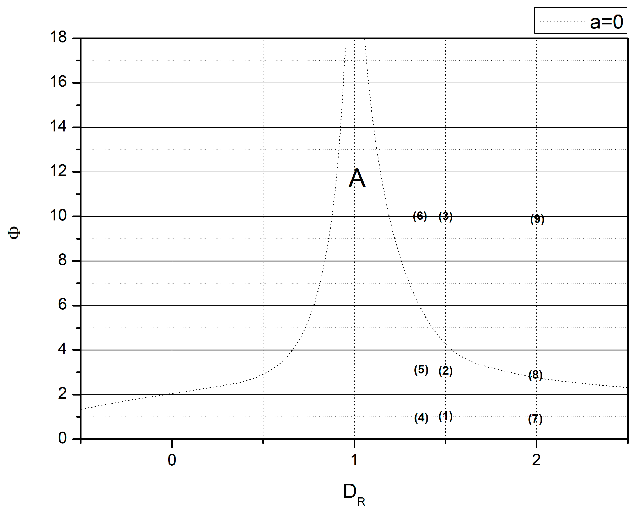
• if Φ = 0.5, then in all cases the point with coordinates (D_R,Φ) lies within the validity region; see Figure 2: points (1), (4), (7);
• if Φ = $\sqrt{10}$, then the point with coordinates (D_R,Φ) lies either in the vicinity of the border of validity region (rows no. 5 and 6) or within (remaining cases); see Figure 2: points (2), (5), (8);
• if Φ = 10, then the point with coordinates (D_R,Φ) lies either in the vicinity of the border of the validity region (row no. 7) or out of it (remaining cases); see Figure 2: points (3), (6), (9).

And

• for Φ = 0.5, in all cases, the effectiveness factor is correctly estimated.
• For Φ = $\sqrt{10}$, in all cases, the effectiveness factor is estimated correctly.
• The Φ = 10 effectiveness factor is correctly estimated only for data presented in row no. 7.

Some observed fluctuations in the applicability range result from the simplicity of the criterion proposed. The single value of the partial derivative does not show trends of a kinetic change (slope), so for many points presented in Table 2, the precision of the model is higher than expected.

Other examples for rectangular geometry of the pellet are presented by Gottifredi et al. [33]. In the first case, the irreversible reaction scheme is A → C. The dimensionless kinetic equation is given by

$$R=c_A^n,$$

(21)

The results are presented in

Table 3. Effectiveness factor for the power-type kinetic equation.

Parameters	ηA	η	ηApM	Error
Φ = 0.5; n = 0.5; DR = 0.5;	0.9602	0.9600	0.9595	0.1%
Φ = 0.8; n = 0.5; DR = 0.5;	0.9048	0.9000	0.9009	−0.1%
Φ = 1.0; n = 0.5; DR = 0.5;	0.8598	0.8495	0.8515	−0.2%
Φ = 1.5; n = 0.5; DR = 0.5;	0.7367	0.7062	0.7097	−0.5%
Φ = 2.0; n = 0.5; DR = 0.5;	0.6196	0.5774	0.5701	1.3%
Φ = 4.0; n = 0.5; DR = 0.5;	0.3288	0.2890	0.2531	12%
Φ = 0.5; n = 1.0; DR = 1.0;	0.9244	0.9242	0.9242	0.0%
Φ = 0.8; n = 1.0; DR = 1.0;	0.8309	0.8300	0.8300	0.0%
Φ = 1.0; n = 1.0; DR = 1.0;	0.7631	0.7616	0.7616	0.0%
Φ = 1.5; n = 1.0; DR = 1.0;	0.6069	0.6034	0.6034	0.0%
Φ = 2.0; n = 1.0; DR = 1.0;	0.4866	0.4820	0.4820	0.0%
Φ = 4.0; n = 1.0; DR = 1.0;	0.2530	0.2498	0.2498	0.0%
Φ = 0.5; n = 1.5; DR = 1.5;	0.8925	0.8926	0.8930	0.0%
Φ = 0.8; n = 1.5; DR = 1.5;	0.7735	0.7766	0.7757	0.1%
Φ = 1.0; n = 1.5; DR = 1.5;	0.6952	0.6996	0.6988	0.1%
Φ = 1.5; n = 1.5; DR = 1.5;	0.5337	0.5400	0.5407	−0.1%
Φ = 2.0; n = 1.5; DR = 1.5;	0.4234	0.4313	0.4322	−0.2%
Φ = 4.0; n = 1.5; DR = 1.5;	0.2212	0.2235	0.2372	−6.1%
Φ = 0.5; n = 2.0; DR = 2.0;	0.8641	0.8644	0.8652	−0.1%
Φ = 0.8; n = 2.0; DR = 2.0;	0.7283	0.7328	0.7322	0.1%
Φ = 1.0; n = 2.0; DR = 2.0;	0.6355	0.6525	0.6515	0.2%
Φ = 1.5; n = 2.0; DR = 2.0;	0.4951	0.5174	0.4978	3.8%
Φ = 2.0; n = 2.0; DR = 2.0;	0.3900	0.4022	0.3988	0.8%
Φ = 4.0; n = 2.0; DR = 2.0;	0.2032	0.2041	0.2255	−11%
Φ = 0.5; n = 3.0; DR = 3.0;	0.8165	0.8180	0.8175	0.1%
Φ = 0.8; n = 3.0; DR = 3.0;	0.6623	0.6641	0.6660	−0.3%
Φ = 1.0; n = 3.0; DR = 3.0;	0.5773	0.5830	0.5838	−0.1%
Φ = 1.5; n = 3.0; DR = 3.0;	0.4264	0.4324	0.4407	−1.9%
Φ = 2.0; n = 3.0; DR = 3.0;	0.3333	0.3364	0.3546	−5.4%
Φ = 4.0; n = 3.0; DR = 3.0;	0.1741	0.1757	0.2067	−17%

. The results obtained by the proposed Gotifredi method are denoted as ηA (column no. 2). The errors presented in column no. 5 relate to an approximate model.

If n = 1.0 then the kinetic equation is linear in nature and the approximate model predicts the effectiveness factor values without errors. In remaining cases, if F < 2 then in all cases the point with coordinates (DR,F) lies within the validity region and the effectiveness factor is correctly estimated. If F = 2 then the point with coordinates (DR,F) lies either in the vicinity of the border of the validity region (for n = 3) or within (remaining cases) and the effectiveness factor is estimated with the error slightly exceeding 5% or correctly, respectively. And finally, if F = 4 then the point with coordinates (DR,F) lies either always out of validity region and the effectiveness factor is estimated incorrectly. The precision of the method proposed by the authors for effective factor estimation and the approximate model (within of its validity range) is similar.

In the second case, the irreversible reaction scheme is A → C. The dimensionless kinetic equation is given by

$$R=\frac{\left(1+K\right)C_A}{1+K{C}_A},$$

(22)

The results are presented in

Table 4. Effectiveness factor for Langmuir–Hinshelwood kinetic equation.

Parameters	ηA	η	ηApM	Error
Φ = 0.1; K = 0.5; DR = 0.667;	0.9974	0.9968	0.9977	−0.1%
Φ = 0.4; K = 0.5; DR = 0.667;	0.9658	0.9638	0.9654	−0.2%
Φ = 0.8; K = 0.5; DR = 0.667;	0.8778	0.8695	0.8716	−0.2%
Φ = 1.0; K = 0.5; DR = 0.667;	0.8232	0.8058	0.8109	−0.6%
Φ = 2.0; K = 0.5; DR = 0.667;	0.5599	0.5183	0.5133	1.0%
Φ = 5.0; K = 0.5; DR = 0.667;	0.2276	0.2130	0.1873	12%
Φ = 0.1; K = 1.0; DR = 0.500;	0.9983	0.9970	0.9983	−0.1%
Φ = 0.4; K = 1.0; DR = 0.500;	0.9741	0.9650	0.9735	−0.9%
Φ = 0.8; K = 1.0; DR = 0.500;	0.8969	0.8922	0.8966	−0.5%
Φ = 1.0; K = 1.0; DR = 0.500;	0.8596	0.8350	0.8426	−0.9%
Φ = 2.0; K = 1.0; DR = 0.500;	0.6179	0.5427	0.5357	1.3%
Φ = 5.0; K = 1.0; DR = 0.500;	0.2531	0.2315	0.1775	23%
Φ = 0.1; K = 5.0; DR = 0.167;	0.9994	0.9970	0.9994	−0.2%
Φ = 0.4; K = 5.0; DR = 0.167;	0.9912	0.9875	0.9908	−0.3%
Φ = 0.8; K = 5.0; DR = 0.167;	0.9658	0.9609	0.9592	0.2%
Φ = 1.0; K = 5.0; DR = 0.167;	0.9475	0.9256	0.9312	−0.6%
Φ = 2.0; K = 5.0; DR = 0.167;	0.5396	0.6174	0.6170	0.1%
Φ = 5.0; K = 5.0; DR = 0.167;	0.2322	0.2480	0.1458	41%

.

The results obtained are similar to those obtained for the power-type kinetic equation. If Φ < 5, then in all cases the point with coordinates (D_R,Φ) lies within the validity region and the effectiveness factor is correctly estimated. In the remaining cases (Φ = 5), the point with coordinates (D_R,Φ) lies without the validity region and the effectiveness factor is incorrectly estimated.

In the third case, the irreversible reaction scheme is A + B → C. The dimensionless kinetic equation is given by

$$R=C_A^n{C}_B^m$$

(23)

The results are presented in

Table 5. Effectiveness factor for power-type kinetic equation for two species.

Parameters	ηA	η	ηApM	Error
Φ = 0.5; n = 0.5; m = 0.5; DR = 0.250;	0.9419	0.9412	0.9416	0.0%
Φ = 0.8; n = 0.5; m = 0.5; DR = 0.250;	0.8657	0.8648	0.8647	0.0%
Φ = 1.0; n = 0.5; m = 0.5; DR = 0.250;	0.8074	0.8057	0.8055	0.0%
Φ = 1.5; n = 0.5; m = 0.5; DR = 0.250;	0.6625	0.6596	0.6570	0.4%
Φ = 2.0; n = 0.5; m = 0.5; DR = 0.250;	0.5408	0.5332	0.5311	0.4%
Φ = 4.0; n = 0.5; m = 0.5; DR = 0.250;	0.2830	0.2799	0.2655	5.1%
Φ = 0.5; n = 0.5; m = 0.5; DR = 0.250;	0.9245	0.9254	0.9249	0.1%
Φ = 0.8; n = 0.5; m = 0.5; DR = 0.250;	0.8315	0.8352	0.8331	0.3%
Φ = 1.0; n = 0.5; m = 0.5; DR = 0.250;	0.7629	0.7683	0.7671	0.2%
Φ = 1.5; n = 0.5; m = 0.5; DR = 0.250;	0.6098	0.6153	0.6156	0.0%
Φ = 2.0; n = 0.5; m = 0.5; DR = 0.250;	0.4910	0.4943	0.4987	−0.9%
Φ = 4.0; n = 0.5; m = 0.5; DR = 0.250;	0.2585	0.2578	0.2669	−3.5%
Φ = 0.5; n = 0.5; m = 0.5; DR = 0.250;	0.8927	0.8948	0.8936	0.1%
Φ = 0.8; n = 0.5; m = 0.5; DR = 0.250;	0.7745	0.7797	0.7779	0.2%
Φ = 1.0; n = 0.5; m = 0.5; DR = 0.250;	0.6969	0.7040	0.7024	0.2%
Φ = 1.5; n = 0.5; m = 0.5; DR = 0.250;	0.5369	0.5462	0.5473	−0.2%
Φ = 2.0; n = 0.5; m = 0.5; DR = 0.250;	0.4263	0.4350	0.4405	−1.3%
Φ = 4.0; n = 0.5; m = 0.5; DR = 0.250;	0.2248	0.2263	0.2458	−8.6%
Φ = 0.5; n = 0.5; m = 0.5; DR = 0.250;	0.8393	0.8412	0.8406	0.1%
Φ = 0.8; n = 0.5; m = 0.5; DR = 0.250;	0.6934	0.6997	0.6976	0.3%
Φ = 1.0; n = 0.5; m = 0.5; DR = 0.250;	0.6094	0.6170	0.6161	0.1%
Φ = 1.5; n = 0.5; m = 0.5; DR = 0.250;	0.4551	0.4631	0.4687	−1.2%
Φ = 2.0; n = 0.5; m = 0.5; DR = 0.250;	0.3575	0.3638	0.3774	−3.7%
Φ = 4.0; n = 0.5; m = 0.5; DR = 0.250;	0.1877	0.1886	0.2188	−16%

.

The results in Table 3, Table 4 and Table 5 confirm the observations presented and conclusions drawn and discussed for the Hougen–Watson kinetic equation (Table 3 and Figure 2). If the values of D_R and Φ are such that the point with coordinates (D_R,Φ) lies within the A-region in Figure 1 (applicability range), the precision of the calculation is high. The relative error is usually a few percent. Out of this range, accuracy goes down, sometimes dramatically. Such examples were intentionally presented in some of the last rows in the single sections in Table 3, Table 4 and Table 5.

Presented here and in previously published papers, the examples confirm the correctness of the presented approximate model. The model is presented in a general form, but it can be easily reduced to a simpler form appropriate to a considered process. The main drawback of the presented model is its limited scope.

4. Conclusions

The approximate models are low-order transient models that can be used for the mathematical description of both steady-state and unsteady-state processes. The model presented in this work is a generalized form of the approximate models presented in [4,5,10]. As other models of linear driving force type, the model presented here makes a simpler analysis of transient and stationary processes in which diffusion in porous media is considered. In contrast to previously published studies, it takes into account the heat balance and mass balances of each component; in each case, the external transfer resistance is taken into consideration. However, it can be easily fitted to any considered process by adjusting the single model parameter, that is, the M modulus. It is able to do so in a very efficient and simple manner, that is, without tedious manipulations of mathematical formulas but by taking into consideration the proper terms in the mentioned modulus M. The terms are directly resulted from the reaction scheme under consideration.

The accuracy of the model is typical for the linear driving force-type approximation of the nonlinear model. At the steady state for sufficiently small Thiele modulus values, the solution of the approximate model approximates well the exact model solution. For the transient solution, the accuracy increases as time passes. The evaluation of the model accuracy is simple; it is based on the information presented here in Figure 1 and the relationship (13).

The proposed approximate model is a simple and handy tool. Within the applicability region, it ensures a simple and precise mathematical tool for both steady-state and unsteady-state analysis of the processes, and it can be used in a very broad range of practical applications, as is noted in the Introduction section.

Some important additional aspects for further investigations should be outlined: (i) the limited range of satisfactory accuracy of nonlinear approximate models should be extended since LDF models are simple and handy tools of process analysis, so a new model is desirable; (ii) the investigations of approximate models concerned processes described by a single reaction; to our best knowledge, such models for multiple reactions have not been derived and presented; and (iii) finding out the applicability range of the approximate model is inconvenient and should be improved.

References

1. Goto, M.; Hirose, T. Approximate rate equation for intraparticle diffusion with or without reaction. Chem. Eng. Sci. 1993, 48, 1912–1915. [Google Scholar] [CrossRef]
2. Kim, D.H. Linear driving force formulas for diffusion and reaction in porous catalysts. AIChE J. 1989, 35, 343–346. [Google Scholar] [CrossRef]
3. Goto, M.; Smith, J.M.; McCoy, B.J. Parabolic profile approximation (linear driving-force model) for chemical reactions. Chem. Eng. Sci. 1990, 45, 443–448. [Google Scholar] [CrossRef]
4. Szukiewicz, M.K. New approximate model for diffusion and reaction in a porous catalyst. AIChE J. 2000, 46, 661–665. [Google Scholar] [CrossRef]
5. Szukiewicz, M.K. Approximate model for diffusion and reaction in a porous catalyst with mass-transfer resistances. AIChE J. 2001, 47, 2131–2135. [Google Scholar] [CrossRef]
6. Başaǧaoǧlu, H.; McCoy, B.J. Linear Driving-Force Model for Diffusion and Reaction with Interphase Partitioning. AIChE J. 2001, 47, 754–756. [Google Scholar] [CrossRef]
7. Álvarez-Ramírez, J.; Valdés-Parada, F.J.; Ochoa-Tapia, J.A. Low-order models for catalyst particles: A dynamic effectiveness factor approach. AIChE J. 2005, 51, 3219–3230. [Google Scholar] [CrossRef]
8. Balakotaiah, V. On the relationship between Aris and Sherwood numbers and friction and effectiveness factors. Chem. Eng. Sci. 2008, 63, 5802–5812. [Google Scholar] [CrossRef]
9. Kim, D.H. Linear driving force formulas for unsteady-state diffusion and reaction in slab, cylinder and sphere catalyst. AIChE J. 2009, 55, 834–839. [Google Scholar] [CrossRef]
10. Szukiewicz, M. An approximate model for diffusion and reaction in a porous pellet. Chem. Eng. Sci. 2002, 57, 1451–1457. [Google Scholar] [CrossRef]
11. Reyes, E.P.; Méndez, A.R.; Escobar, G.V.; Rugerio, C.G. Approximate Solution to the Diffusion-Reaction Problem with Nonlinear Kinetics in Transient Systems. In Innovations and Advanced Techniques in Computer and Information Sciences and Engineering; Sobh, T., Ed.; Springer: Dordrecht, The Netherlands, 2007; pp. 133–138. [Google Scholar] [CrossRef]
12. Szukiewicz, M.; Petrus, R. Approximate model for diffusion and reaction in a porous pellet and an effectiveness factor. Chem. Eng. Sci. 2004, 59, 479–483. [Google Scholar] [CrossRef]
13. Bidabehere, C.M.; García, J.R.; Sedran, U. Transient effectiveness factor in porous catalyst particles. Application to kinetic studies with batch reactors. Chem. Eng. Res. Des. 2017, 118, 41–50. [Google Scholar] [CrossRef]
14. Valencia, P.; Ibañez, F. Estimation of the effectiveness factor for immobilized enzyme catalysts through a simple conversion assay. Catalysts 2019, 9, 930. [Google Scholar] [CrossRef]
15. Mary, M.L.C.; Devi, M.C.; Meena, A.; Rajendran, L.; Abukhaled, M. Mathematical modeling of immobilized enzyme in porous planar, cylindrical, and spherical particle: A reliable semi-analytical approach. React. Kinet. Mech. Catal. 2021, 134, 641–651. [Google Scholar] [CrossRef]
16. Abu-Reesh, I.M. Approximation of intra-particle reaction/diffusion effects of immobilized enzyme system following reverse Michaelis–Menten (rMM) mechanism: Third degree polynomial and Akbari–Ganji methods. React. Kinet. Mech. Catal. 2023, 136, 2875–2892. [Google Scholar] [CrossRef]
17. Ananthaswamy, V.; Rajendran, L. Approximate analytical solution of non-linear kinetic equation in a porous pellet. Glob. J. Pure Appl. Math. 2012, 8, 101–111. [Google Scholar]
18. Gwadera, M.; Kupiec, K.; Neupauer, K. Approximate equations of mass diffusion and heat conduction with a source term. Przem. Chem. 2016, 95, 1988–1993. [Google Scholar]
19. Skoneczny, S.; Cioch-Skoneczny, M. Mathematical modelling and approximate solutions for microbiological processes in biofilm through homotopy-based methods. Chem. Eng. Res. Des. 2018, 139, 309–320. [Google Scholar] [CrossRef]
20. Bizon, K. Assessment of a POD method for the dynamical analysis of a catalyst pellet with simultaneous chemical reaction, adsorption and diffusion: Uniform temperature case. Comp. Chem. Eng. 2017, 97, 259–270. [Google Scholar] [CrossRef]
21. Bizon, K.; Tabiś, B. Adsorption with chemical reaction in porous catalyst pellets under alternate concentration fields. Uniform temperature case. Chem. Proc. Eng. 2016, 37, 473–484. [Google Scholar] [CrossRef]
22. Bizon, K.; Tabiś, B. Dynamics of an isothermal catalyst pellet with simultaneous chemical reaction and adsorption. Chem. Eng. Res. Des. 2016, 115, 221–229. [Google Scholar] [CrossRef]
23. Georgiou, A. Asymptotically exact driving force approximation for intraparticle mass transfer rate in diffusion and adsorption processes: Nonlinear isotherm systems with macropore diffusion control. Chem. Eng. Sci. 2004, 59, 3591–3600. [Google Scholar] [CrossRef]
24. Georgiou, A.; Kupiec, K. Nonlinear driving force approximations for intraparticle mass transfer in adsorption processes. Nonlinear isotherm systems with macropore diffusion control. Chem. Eng. J. 2003, 92, 185–191. [Google Scholar] [CrossRef]
25. Szukiewicz, M.; Petrus, R. Approximate models application for modelling of fixed bed reactors. Hung. J. Ind. Chem. 2001, 29, 91–94. [Google Scholar]
26. Pereira, C.S.M.; Gomes, P.S.; Gandi, G.K.; Silva, V.M.T.M.; Rodrigues, A.E. Multifunctional reactor for the synthesis of dimethylacetal. Ind. Eng. Chem. Res. 2008, 47, 3515–3524. [Google Scholar] [CrossRef]
27. Bidabehere, C.M.; García, J.R.; Sedran, U. Transient effectiveness factors in the dynamic analysis of heterogeneous reactors with porous catalyst particles. Chem. Eng. Sci. 2015, 137, 293–300. [Google Scholar] [CrossRef]
28. Sá Gomes, P.; Leão, C.P.; Rodrigues, A.E. Simulation of true moving bed adsorptive reactor: Detailed particle model and linear driving force approximations. Chem. Eng. Sci. 2007, 62, 1026–1041. [Google Scholar] [CrossRef]
29. Pietschak, A.; Kaiser, M.; Freund, H. Tailored catalyst pellet specification for improved fixed-bed transport characteristics: A shortcut method for the model-based reactor design. Chem. Eng. Res. Des. 2018, 137, 60–74. [Google Scholar] [CrossRef]
30. Skoneczny, S.; Cioch-Skoneczny, M. Approximate Models of Microbiological Processes in a Biofilm Formed on Fine Spherical Particles. Processes 2022, 10, 48. [Google Scholar] [CrossRef]
31. Kumar, J.; Kukreja, V.K. Analytic solution of a diffusion dispersion model of packed bed of finite thickness. J. Interdiscip. Math. 2019, 22, 1–16. [Google Scholar] [CrossRef]
32. Belfiore, L.A. Transport Phenomena for Chemical Reactor Design; John Wiley & Sons: Hoboken, NJ, USA, 2003; pp. 491–508. [Google Scholar]
33. Gottifredi, J.C.; Gonzo, E.E.; Quiroga, O.D. Isothermal Effectiveness Factor I. Analytical expression for single reaction with arbitrary kinetics. Slab geometry. Chem. Eng. Sci. 1981, 36, 705–711. [Google Scholar]
Figure 1. Applicability range of ApM for different geometries of the pellet. Curves were calculated numerically for negligible external transfer resistances.
Reactions 05 00015 g001