Coupled Temperature–Humidity Modeling and Dual-Loop Fuzzy-PID Regulation for an Edible Fungi Cultivation Room

Abstract

Maintaining stable temperature and relative humidity (RH) is essential for edible fungi cultivation, yet indoor climates exhibit nonlinear, coupled thermal–moisture dynamics that can degrade disturbance rejection and increase energy use. This study proposes a reproducible lumped-parameter temperature–humidity model and evaluates a dual-loop (SISO × 2) fuzzy-PID regulation strategy in MATLAB/Simulink under standardized simulation scenarios. The model formulates energy and moisture conservation using physically interpretable parameters (air mass, ventilation exchange, heat transfer, and actuator limits), with RH obtained from a psychrometric transformation of humidity ratio. Three benchmark tests are designed for repeatable assessment: set-point tracking, step disturbances (±2 °C and ±5% RH), and periodic disturbances. A Simulated Growth Indicator (SGI) is introduced as a phenomenological model representing potential growth trends under controlled temperature and humidity, rather than actual measured crop yield. The fuzzy-PID strategy is compared with conventional PID and a no-control baseline using unified performance metrics (steady-state deviation, recovery/settling behavior, integral error) and actuator energy consumption computed from explicit power models. Results show that fuzzy-PID achieves faster recovery and lower error accumulation than PID under identical disturbances while reducing total energy consumption (e.g., 5.7 kWh vs. 6.7 kWh in a representative case). Although the plant is dynamically coupled, the controller implementation remains a practical dual-loop structure; the presented framework therefore serves as a reproducible simulation benchmark for controller comparison in high-humidity cultivation stages.

1. Introduction

Edible fungi cultivation has become increasingly important due to its nutritional and medicinal value, as well as its significant economic impact. Maintaining a stable microclimate is therefore critical, as yield and quality are highly sensitive to environmental fluctuations. In particular, temperature and relative humidity (RH) are the most critical controllable variables, and maintaining them within appropriate ranges is essential throughout the long cultivation cycles. However, the indoor environment is governed by nonlinear heat and moisture transfer processes, external disturbances (e.g., ventilation and ambient variations), and actuator constraints, which may result in slow dynamic responses, steady-state deviations, and increased energy consumption [1].

Previous studies have addressed temperature and humidity control in agricultural environments with varying approaches. For example, investigated the impact of temperature and humidity regulation on crop growth but did not consider the nonlinear coupling between these variables. proposed an adaptive PID method, yet its performance in disturbance rejection and energy efficiency was limited. applied classical PID control, but the study did not account for real-time control constraints typical of small-scale cultivation chambers. These limitations highlight the need for a control strategy that can handle coupled dynamics, provide robust disturbance rejection, and remain feasible for real-time implementation.

A significant engineering challenge lies in the intrinsic coupling between temperature and RH. Temperature variations alter the air’s moisture-holding capacity, which in turn affects RH, while humidification and ventilation processes modify moisture content and simultaneously influence thermal conditions. As a result, controlling temperature and humidity independently may induce cross-effects, degrade disturbance rejection, and complicate system stability. These complex, interrelated dynamics necessitate the development of an advanced modeling and control framework that can be evaluated under standardized and reproducible conditions. Addressing this need is crucial to improving the stability of the cultivation environment and reducing energy consumption [2,3].

Currently, traditional PID controllers are widely used for temperature and humidity regulation in cultivation systems. However, due to the nonlinear coupling between temperature and humidity, fixed-parameter PID control often struggles to reject disturbances effectively and maintain a stable environment. In particular, the temperature and humidity dynamics interact in such a way that independent control of each variable can lead to cross-effects, reducing the overall system performance. Advanced methods, such as model predictive control (MPC) and adaptive control (AC), have been proposed to address these challenges, but these strategies often require accurate system models and substantial computational resources. Consequently, their application is often limited in small- to medium-scale cultivation environments, where computational power and resources may be constrained. This study aims to develop a fuzzy-PID-based control strategy to address the challenges posed by the coupling between temperature and humidity in edible fungi cultivation. By adjusting the control increment based on the error and its variation, the fuzzy-PID controller can improve disturbance rejection and recovery performance without requiring an exact mathematical model of the system. This flexibility makes fuzzy-PID less dependent on model precision and computational resources compared to advanced multivariable methods like MPC or AC, making it particularly suitable for small- and medium-scale cultivation facilities.

The objective of this work is to provide a reproducible simulation-based benchmark for controller assessment. Unlike more advanced methods that claim global optimality, this study evaluates fuzzy-PID as an intermediate solution between classical PID and model-based multiple-input multiple-output (MIMO) approaches. This paper compares fuzzy-PID with traditional PID control through reproducible numerical experiments in MATLAB/Simulink and evaluates their performance using a new Simulated Growth Indicator (SGI). Furthermore, an energy consumption analysis is conducted to assess the potential energy savings of the proposed approach. The main contributions of this study include: ① Development of a coupled temperature–humidity dynamic model based on physical principles; ② Proposal of a dual-loop fuzzy-PID control strategy (SISO × 2 structure) for regulating temperature and humidity; ③ Introduction of a Simulated Growth Indicator (SGI) to evaluate the performance of different control strategies; ④ Comprehensive evaluation of energy consumption under different control methods to assess their energy efficiency.

2. Related Work and Contribution Statement

In recent years, many studies have proposed models for temperature and humidity control, with PID control methods being the most commonly used. However, traditional PID controllers often struggle to achieve effective disturbance rejection when dealing with the coupled dynamics between temperature and humidity. This limitation arises from the inherent nonlinearity of the temperature–humidity relationship, where independent control of each variable may lead to cross-effects that degrade system performance.

To overcome these limitations, some studies have explored multivariable control approaches, such as Model Predictive Control (MPC) and Adaptive Control (AC). These methods are better designed to handle the complex interactions between temperature and humidity. However, MPC and AC typically rely on detailed system models and require significant computational resources, making them less practical for small- to medium-scale cultivation facilities where real-time processing capabilities and system complexity are limited [4,5].

Fuzzy control methods have also been investigated in agricultural environments as a potential solution to nonlinearities and uncertainties. Fuzzy-PID controllers, in particular, offer a promising approach by adjusting control increments based on error and its variation, which enhances robustness and disturbance rejection without requiring precise system models [6]. The fuzzy-PID method has been shown to perform well in environments with nonlinear, coupled dynamics, offering a simpler, more computationally efficient alternative to more complex methods such as MPC and AC. While these methods each offer distinct advantages, they also come with limitations in terms of complexity, computational demands, and scalability. This research builds upon these previous efforts by introducing a dual-loop fuzzy-PID controller that combines the strengths of fuzzy logic with PID control to provide an effective and efficient solution for temperature and humidity regulation in small- to medium-scale edible fungi cultivation systems.

The main contributions of this study are as follows: ① Development of a coupled temperature–humidity dynamic model: This model effectively simulates the nonlinear coupling between air temperature and relative humidity, accounting for their complex interactions and providing a foundation for control strategies. ② Introduction of a dual-loop fuzzy-PID control method: This method enhances system robustness under temperature and humidity disturbances by leveraging fuzzy logic to adjust control increments, thus improving disturbance rejection and system stability [7,8]. ③ Design of a Simulated Growth Indicator (SGI): The SGI is used to evaluate the environmental stability of different control strategies, offering a new metric for assessing the effectiveness of temperature and humidity regulation in cultivation systems. ④ Energy consumption analysis: A comprehensive energy evaluation model is introduced to assess and compare the energy efficiency of different control strategies, highlighting the potential for reducing energy consumption in temperature and humidity regulation. These contributions provide an innovative solution for effective temperature and humidity control in edible fungi cultivation environments, improving both system performance and energy efficiency.

3. Analysis of Temperature and Humidity Requirements and Coupling Mechanism for Edible Fungi Growth

3.1. Growth Stages of Edible Fungi and Environmental Requirements

The cultivation process of edible fungi can be generally described by several stages (e.g., germination, mycelial growth, fruiting, and maturation), and the environmental requirements may vary across stages and species. To ensure reproducibility in this paper, we focus on a representative high-humidity cultivation condition used in the subsequent control tests and set the set-points to T = 22 °C and RH = 90% throughout the simulation study. This setting enables consistent comparisons of different control strategies under identical operating conditions and disturbance profiles, underscoring the need for precise, coordinated regulation of temperature and relative humidity to improve cultivation performance.

3.2. Physical Relationship and Coupling Characteristics Between Temperature and Relative Humidity

There exists a close physical coupling relationship between temperature and relative humidity. Temperature affects the air’s saturation capacity for water vapor, while relative humidity depends on both temperature and the actual water vapor content. Specifically, relative humidity (RH) can be expressed as the ratio of the actual water vapor pressure $e_s\left(T\right)$ at the same temperature:

$$RH={\displaystyle \frac{e}{e_s\left(T\right)}}\times 100\%$$

(1)

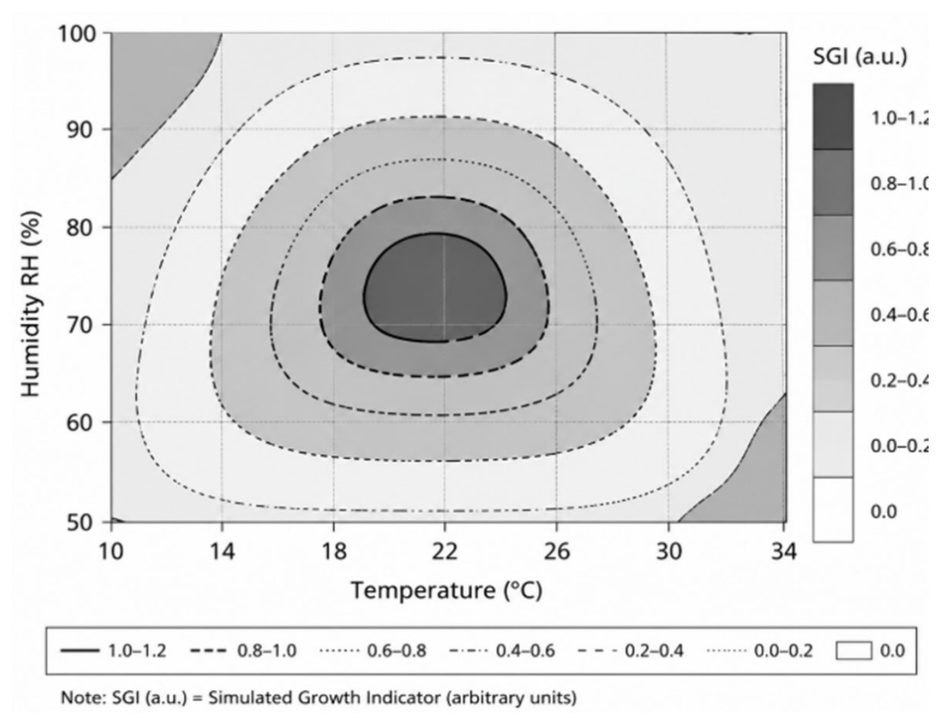
where e is the actual vapor pressure and ${\mathrm{e}}_{\mathrm{s}}\left(\mathrm{T}\right)$ is the saturation vapor pressure at temperature T. As temperature changes, ${\mathrm{e}}_{\mathrm{s}}\left(\mathrm{T}\right)$ changes nonlinearly, so RH may vary significantly even when the absolute moisture content is unchanged. In edible fungi cultivation, such coupling means that regulating temperature can alter RH, and humidification/ventilation can also influence thermal conditions. Therefore, controlling a single factor independently may lead to cross-effects and make it difficult to maintain an optimal growth environment under disturbances; both factors should be considered jointly in control. Contour map of the simulated growth-response surface as a function of temperature (°C) and relative humidity (%). The optimal region corresponds to the assumed set-point (22 °C, 90% RH). The color bar represents the normalized predicted growth indicator (dimensionless). Simulation parameters follow those listed in Figure 1.

The humidity state can be characterized using the humidity ratio w (kg water vapor per kg dry air):

$$w=0.622{\displaystyle \frac{p_v}{p_{atm}-p_v}}$$

(2)

where p_atm is the atmospheric pressure (Pa), and p_v is the water vapor partial pressure (Pa). In the dynamic model developed in this study, the internal state variables are temperature T and humidity ratio w, while RH is calculated as an output variable through psychrometric transformation.

For reproducible implementation in MATLAB/Simulink, the vapor pressure is obtained from the humidity ratio using the inverse relationship of Equation (2):

$$p_v={\displaystyle \frac{p_{atm}w}{0.622+w}}$$

(3)

The saturation vapor pressure psat(T) is calculated using the Tetens correlation:

$${\mathrm{p}}_{\mathrm{s}\mathrm{a}\mathrm{t}}\left(\mathrm{T}\right)=610.78\mathrm{e}\mathrm{x}\mathrm{p}\left({\displaystyle \frac{17.2694\mathrm{T}}{\mathrm{T}+237.3}}\right)$$

(4)

where psat(T) is expressed in Pa and T is the air temperature in °C. This empirical correlation is valid approximately within the temperature range of 0–50 °C, which covers the operating conditions considered in this study.

The complete computational sequence used in the MATLAB/Simulink simulation is therefore:

$$\mathrm{w}{\top }_{\mathrm{v}}{\top }_{\mathrm{s}\mathrm{a}\mathrm{t}}\left(\mathrm{T}\right)\to \mathrm{R}\mathrm{H}$$

where the relative humidity output is calculated as:

$$RH={\displaystyle \frac{p_v}{p_{sat}\left(T\right)}}\times 100\%$$

(5)

This calculation procedure ensures that RH is obtained consistently from the conserved moisture state and temperature state, rather than being independently modeled as a dynamic variable.

Equations (2)–(5) demonstrate that RH depends jointly on temperature T and humidity ratio w. Therefore, even if the absolute moisture content remains constant, variations in temperature modify p_sat(T), resulting in nonlinear changes in RH. From a dynamic perspective, the temperature–humidity coupling arises from two fundamental mechanisms:

(1)

Moisture mass balance

The indoor humidity ratio evolves according to water vapor conservation:

$$m_a{\displaystyle \frac{dw}{dt}}={\dot{m}}_{hum}+{\dot{m}}_{evap}-{\dot{m}}_{vent}\left(w-w_{amb}\right)-{\dot{m}}_{dehum}$$

(6)

where m_a is the air mass in the room, ${\dot{m}}_{hum}$ is the humidification input, ${\dot{m}}_{evap}$ represents evaporation from substrates, ${\dot{m}}_{vent}$ is the ventilation mass flow rate, $w_{amb}$ is the ambient humidity ratio, and ${\dot{m}}_{dehum}$ denotes dehumidification effects. This equation governs the evolution of water vapor content independently of temperature.

(2)

Latent heat coupling in the energy balance

Phase change in moisture introduces latent heat effects into the thermal dynamics. The temperature equation, therefore, includes a latent heat term:

$$m_a{c}_p{\displaystyle \frac{dT}{dt}}=Q_{heater}-UA\left(T-T_{amb}\right)-{\dot{m}}_{vent}{c}_p\left(T-T_{amb}\right)\pm L_v{\dot{m}}_{evap}$$

(7)

where $c_p$ is the specific heat capacity of air, UA is the overall heat transfer coefficient, $L_v$ is the latent heat of vaporization, and ${\dot{m}}_{evap}$ represents a moisture phase change. The term $L_v{\dot{m}}_{evap}$ explicitly couples moisture dynamics to temperature dynamics, since evaporation absorbs heat while condensation releases heat.

These relationships indicate that RH is not an independent thermodynamic state variable but a nonlinear function of temperature and moisture content. The moisture balance determines the evolution of humidity ratio w, while temperature variations modify the saturation vapor pressure p_sat(T). The interaction between these two mechanisms produces the nonlinear temperature–humidity coupling observed in cultivation environments.

In the present study, the environmental dynamic model is therefore formulated using temperature T and humidity ratio w as the fundamental state variables to satisfy physical conservation principles. Relative humidity is calculated from these states through the psychrometric transformation described above and is used as the controlled output variable in the feedback control system. This formulation ensures physical consistency and provides a fully reproducible implementation framework for MATLAB/Simulink simulations.

3.3. Mechanism Model of the Effect of Temperature and Humidity on Mycelial Growth

In this study, the growth-rate function r(T, H) is introduced as a phenomenological, illustrative model to describe the qualitative effects of temperature and humidity on mycelial development. The adopted Gaussian-type expression reflects the widely observed biological tendency that growth decreases when environmental variables deviate from their optimal ranges.

It should be clearly stated that the Gaussian form adopted in this paper is an assumed response model constructed for simulation purposes. The parameters (e.g., optimal temperature, optimal humidity, and sensitivity coefficients) are selected to represent typical high-humidity cultivation conditions reported in the literature, but they are not derived from a specific experimental dataset nor calibrated against measured growth data. The model is therefore not intended for quantitative prediction of actual growth rate or yield.

Instead, the growth function is used as a simulation-based indicator that maps environmental deviations to a Simulated Growth Indicator (SGI), enabling relative comparison of control strategies under identical disturbance conditions. Consequently, the model serves as a theoretical linkage between environmental stability and biological suitability, rather than a validated biological growth prediction model.

4. Construction of the Temperature–Humidity Coupling Mathematical Model

4.1. Construction of the Environmental Temperature–Humidity Dynamics Model

To ensure physical consistency and reproducibility, the cultivation room is modeled as a well-mixed control volume. The control-volume boundary encloses the indoor air only, while the cultivation substrates, walls, racks, and other structural components are not included in the air-energy storage term. The state variables are the indoor air temperature T and humidity ratio w. The air mass is defined as

$$m_a=\rho V$$

(8)

where (V) is the room volume (m³) and ($\rho$) is the air density (kg/m³).

(1)

Temperature dynamics

The thermal energy balance of the room air is expressed as

$$m_a{c}_p\dot{T}=Q_{heater}-UA\left(T-T_{amb}\right)-{\dot{m}}_v{c}_p\left(T-T_{amb}\right)+L_v{\dot{m}}_{evap}+Q_{int}$$

(9)

where $c_p$ is the specific heat capacity of air (J·kg⁻¹·K⁻¹), $UA$ is the overall heat transfer coefficient (W·K⁻¹), ${\dot{m}}_v$ is the ventilation mass flow rate (kg·s⁻¹), $L_v$ is the latent heat of vaporization (J·kg⁻¹), $Q_{heater}$ is the heating input (W), and $Q_{int}$ represents internal heat gains.

In the adopted sign convention, ${\dot{m}}_{\mathrm{e}\mathrm{v}\mathrm{a}\mathrm{p}}$ > 0 represents evaporation from the cultivation substrate into the indoor air. Because evaporation consumes sensible heat, its contribution to the indoor air-energy balance is represented by the cooling term

$$-L_v{\dot{m}}_{\mathrm{e}\mathrm{v}\mathrm{a}\mathrm{p}}<0.$$

Conversely, ${\dot{m}}_{\mathrm{e}\mathrm{v}\mathrm{a}\mathrm{p}}$ < 0 represents net condensation of water vapor from the air. Under this condition,

$$-L_v{\dot{m}}_{\mathrm{e}\mathrm{v}\mathrm{a}\mathrm{p}}>0,$$

which represents the release of latent heat during condensation. Therefore, ${\dot{m}}_{\mathrm{e}\mathrm{v}\mathrm{a}\mathrm{p}}$ is defined as a signed net phase-change flux rather than as a strictly positive evaporation-only term. This convention is used consistently in both the temperature and moisture balances.

The enthalpy associated with phase change is not represented by an additional vapor-enthalpy source term. Instead, the thermal effect of evaporation or condensation is included exclusively through the term

$$-L_v{\dot{m}}_{\mathrm{e}\mathrm{v}\mathrm{a}\mathrm{p}},$$

Thereby avoiding double counting. The electrical energy consumption of the active humidifier is evaluated separately in the actuator energy model. Because the present air-energy balance does not explicitly model the sensible heat exchange between supplied water droplets and indoor air, no additional latent-heat term associated with the humidifier moisture input is included in Equation (9).

The effective thermal capacity previously denoted as C_T is therefore explicitly defined as

$$C_T=m_a{c}_p$$

(10)

(2)

Moisture dynamics

The moisture balance is formulated as

$$m_a{\displaystyle \frac{dw}{dt}}={\dot{m}}_{\mathrm{h}\mathrm{u}\mathrm{m}}+{\dot{m}}_{\mathrm{e}\mathrm{v}\mathrm{a}\mathrm{p}}-{\dot{m}}_v\left(w-w_{\mathrm{a}\mathrm{m}\mathrm{b}}\right)-{\dot{m}}_{\mathrm{d}\mathrm{e}\mathrm{h}\mathrm{u}\mathrm{m}}$$

(11)

where ${\dot{m}}_{hum}$ is the humidification input (kg·s⁻¹), ${\dot{m}}_{evap}$ is evaporation from substrates, $w_{amb}$ is the ambient humidity ratio, and ${\dot{m}}_{dehum}$ denotes dehumidification. According to the adopted sign convention, a positive ${\dot{m}}_{\mathrm{e}\mathrm{v}\mathrm{a}\mathrm{p}}$ increases the indoor humidity ratio, whereas a negative ${\dot{m}}_{\mathrm{e}\mathrm{v}\mathrm{a}\mathrm{p}}$ represents condensation and decreases the vapor content of the indoor air. The same signed definition is therefore used in Equations (9) and (11), ensuring consistency between the energy and moisture conservation equations. The effective moisture capacity is thus.

$$C_H=m_a$$

(12)

which reflects the mass of air governing vapor storage.

(3)

Actuator characteristics

Control inputs are mapped to physical quantities through linear gains with saturation constraints:

$$Q_{heater}=K_h{u}_h,\hspace{1em}{\dot{m}}_{hum}=K_m{u}_m$$

(13)

where $u_h$, $u_m$∈ in [0, 1]) are normalized control signals, and K_h, $K_m$ are actuator gains. Saturation limits and optional first-order actuator dynamics can be included as

$${\tau }_a\dot{u}+u=u_{cmd}$$

(14)

where u_cmd is the commanded normalized control signal, u is the actual actuator output, and τ_a is the actuator time constant. Saturation is applied after the dynamic response to ensure that the actual actuator signal remains within the physical interval.

$$0\le u\le 1$$

4.2. Coupled Temperature–Humidity Growth Model and System Coupling Structure Design

The impact of temperature and humidity on the growth of edible fungi should be comprehensively characterized using a system-level coupling model [9,10]. Based on the growth-rate relationship described in Section 3.3 and the temperature–humidity dynamic equations in Section 4.1, a coupled temperature–humidity growth model can be constructed by treating environmental temperature and humidity as system inputs and the mycelial growth rate as the output. The coupled model can be written in a compact form as:

$$r\left(t\right)=f\left(\mathrm{T}\left(\mathrm{t}\right),\mathrm{H}\left(\mathrm{t}\right)\right)$$

(15)

where $r\left(t\right)$ is the mycelial growth rate and $f\left(•\right)$ represents the coupled effect of dynamic temperature and humidity on growth.

For the system coupling structure, the control objective is to regulate $T\left(t\right)$ and $H\left(t\right)$ (or RH) to their set-points under disturbances, so that r(t) remains close to its optimal region. In practice, the coupling structure should include sensor feedback (temperature and humidity measurements), a controller that computes control actions (heating/humidification/ventilation), and the dynamic model that describes how the environment responds to control inputs and external disturbances. This closed-loop coupling structure supports real-time adjustment of temperature and humidity to maintain a favorable growth environment and improve cultivation performance [11,12,13].

5. Temperature–Humidity Coupling Control Strategy Design

5.1. Analysis of the MIMO (Multiple Input Multiple Output) Control System

Although the temperature–humidity dynamics are intrinsically coupled, the control implementation in this study adopts a practical dual-loop (SISO × 2) structure. The coupling exists in the plant (environmental dynamics), while the temperature and humidity controllers are implemented as two coordinated but independent loops. This engineering approach is widely used in practice due to its simplicity and ease of implementation. The controllers do not explicitly perform model-based decoupling; instead, robustness is enhanced through fuzzy supervision to mitigate cross-effects under disturbances.

The temperature–humidity coupling system can be regarded as a multivariable regulation problem because temperature and relative humidity are distinct variables but exhibit strong cross-effects. In such systems, independent adjustment of one variable may inadvertently perturb the other, increasing control difficulty and motivating coordinated regulation. Therefore, the controller design should explicitly account for the interaction between temperature and humidity to reduce cross-coupling and improve disturbance rejection [14].

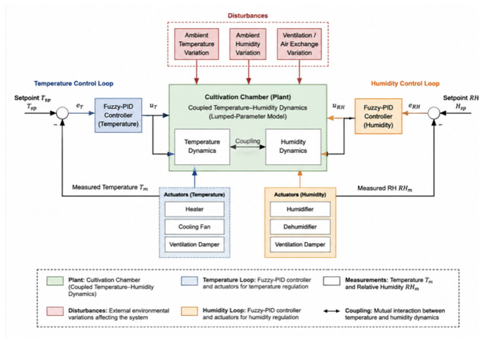
In this study, a lumped-parameter model is adopted rather than a distributed model based on partial differential equations (PDEs). This choice is justified by the relatively uniform temperature and humidity distribution in small-scale cultivation chambers, as well as the computational complexity and real-time limitations associated with PDE-based models. For larger-scale cultivation environments or cases with significant spatial gradients, PDE-based distributed models may be considered in future work. In principle, advanced multivariable methods (e.g., model predictive control and adaptive control) can be used to coordinate coupled variables when a sufficiently accurate model and constraints are available. However, to provide a reproducible and implementable baseline, this study focuses on comparing classical PID and fuzzy-PID strategies under standardized simulation scenarios, while leaving advanced multivariable optimization for extension [15,16]. The overall architecture of the dual-loop temperature–humidity control system is illustrated in Figure 2.

5.2. Reproducible Design of the Fuzzy–PID Controller

To improve robustness under nonlinear temperature–humidity coupling, a fuzzy-supervised incremental PID structure is adopted. For consistency, both the baseline PID controller and the fuzzy-PID controller are implemented in incremental form, thereby ensuring a fair comparison under identical sampling intervals, actuator constraints, and disturbance conditions.

(1)

Controller structure

For each control loop, the tracking error and its first-order difference are defined as

$$e\left(k\right)=r\left(k\right)-y\left(k\right),\hspace{1em}\Delta e\left(k\right)=e\left(k\right)-e\left(k-1\right)$$

(16)

where r(k) is the reference value, y(k) is the measured output, e(k) is the tracking error, and Δe(k) is the change in the tracking error at sampling instant k.

The fuzzy inference system generates a normalized incremental output Δu_n(k). The actual actuator command is updated according to

$$u\left(k\right)=\mathrm{s}\mathrm{a}\mathrm{t}\left[u\left(k-1\right)+K_u\Delta u_n\left(k\right)\right]$$

(17)

where K_u is the output scaling factor and sat(⋅) is the saturation function defined as

$$\mathrm{s}\mathrm{a}\mathrm{t}\left(x\right)=\mathrm{m}\mathrm{i}\mathrm{n}\left[u_{\mathrm{m}\mathrm{a}\mathrm{x}},\mathrm{m}\mathrm{a}\mathrm{x}\left(u_{\mathrm{m}\mathrm{i}\mathrm{n}},x\right)\right]$$

(18)

In this study, the actuator command is normalized and constrained by

$$u_{\mathrm{m}\mathrm{i}\mathrm{n}}=0,\hspace{1em}{u}_{\mathrm{m}\mathrm{a}\mathrm{x}}=1$$

(19)

Thus, u(k) is a dimensionless normalized actuator command. For the temperature loop, u_T = 0 indicates that the heater is switched off, whereas u_T = 1 corresponds to operation at the rated heating power. For the humidity loop, u_RH = 0 indicates that the humidifier is switched off, whereas u_RH = 1 corresponds to the maximum humidification rate.

(2)

Input/output scaling factors

The fuzzy inputs are normalized to ([−1, 1]):

$$e_n=K_{e}e,\hspace{1em}\Delta e_n=K_d\Delta e$$

(20)

where $K_e$ and $K_d$ are the input scaling factors for the tracking error and error variation, respectively. Values outside the normalized input range are limited to [−1, 1] before fuzzy inference. The adopted input scaling factors are

$$\mathrm{Temperature} \mathrm{loop}:{\mathrm{K}}_{\mathrm{e}}^{\mathrm{T}}=1/3, {\mathrm{K}}_{\mathrm{d}}^{\mathrm{T}}=1/2$$

$$\mathrm{Humidity} \mathrm{loop}: {\mathrm{K}}_{\mathrm{e}}^{\mathrm{R}\mathrm{H}}=1/8, {\mathrm{K}}_{\mathrm{d}}^{\mathrm{R}\mathrm{H}}=1/5$$

The fuzzy output is also defined over the normalized universe of discourse

$$\Delta u_n\left(k\right)\in \left[-1,1\right]$$

(21)

where Δu_n(k) is dimensionless. It is converted into the actual normalized control increment using

$$\Delta u_{\mathrm{a}\mathrm{c}\mathrm{t}\mathrm{u}\mathrm{a}\mathrm{l}}\left(k\right)=K_u\Delta u_n\left(k\right)$$

(22)

Because the heater and humidifier have different physical capacities and dynamic characteristics, separate output scaling factors are adopted:

$$K_{u,T}=0.02,\hspace{1em}{K}_{u,RH}=0.03$$

(23)

Therefore, the two actuator commands are updated as

$$u_T\left(k\right)=\mathrm{s}\mathrm{a}\mathrm{t}\left[u_T\left(k-1\right)+K_{u,T}\Delta u_{n,T}\left(k\right)\right]$$

(24)

and

$$u_{RH}\left(k\right)=\mathrm{s}\mathrm{a}\mathrm{t}\left[u_{RH}\left(k-1\right)+K_{u,RH}\Delta u_{n,RH}\left(k\right)\right]$$

(25)

The selected values imply that the normalized heater command can change by at most 0.02 during one sampling interval, whereas the normalized humidifier command can change by at most 0.03 during one sampling interval.

The normalized commands are subsequently mapped to physical actuator outputs as

$$Q_{\mathrm{h}\mathrm{e}\mathrm{a}\mathrm{t}\mathrm{e}\mathrm{r}}\left(k\right)=P_{\mathrm{r}\mathrm{a}\mathrm{t}\mathrm{e}\mathrm{d}}{u}_T\left(k\right)$$

(26)

and

$${\dot{m}}_{\mathrm{h}\mathrm{u}\mathrm{m}}\left(k\right)={\dot{m}}_{\mathrm{h}\mathrm{u}\mathrm{m},\mathrm{m}\mathrm{a}\mathrm{x}}{u}_{RH}\left(k\right)$$

(27)

where

$$P_{\mathrm{r}\mathrm{a}\mathrm{t}\mathrm{e}\mathrm{d}}=3000 \mathrm{W}$$

is the rated heater power and

$${\dot{m}}_{\mathrm{h}\mathrm{u}\mathrm{m},\mathrm{m}\mathrm{a}\mathrm{x}}=0.002 \mathrm{k}\mathrm{g}{\mathrm{s}}^{-1}$$

is the maximum humidification mass-flow rate.

The scaling and actuator parameters used in the simulation are summarized in

Table 1. Input/output scaling and actuator constraints of the fuzzy-PID controller.

Parameter	Temperature Loop	Humidity Loop
Error input universe	([−1, 1])	[−1, 1]
Error-change input universe	([−1, 1])	[−1, 1]
Output universe (Δun)	([−1, 1])	[−1, 1]
Error scaling factor (Ke)	(1/3)	(1/8)
Error-change scaling factor (Kd)	(1/2)	(1/5)
Output scaling factor (Ku)	0.02	0.03
Normalized actuator range	([0, 1])	([0, 1])
Physical actuator range	0–3000 W	0–0.002 kg, s−1
Sampling interval (Ts)	1 s	1 s

.

(3)

Membership functions

Five linguistic variables are used:

$$\{NB,NS,ZO,PS,PB\}$$

Triangular membership functions are uniformly distributed over ([−1, 1]):

NB: (−1, −1, −0.5)

NS: (−1, −0.5, 0)

ZO: (−0.5, 0, 0.5)

PS: (0, 0.5, 1)

PB: (0.5, 1, 1)

Each triplet denotes (left, center, right) points of the triangle.

Design rationale: The membership functions are defined as uniformly distributed triangular functions, with center and boundary points set based on empirical rules to cover the input range [−1, 1]. The parameters were adjusted through simulation experiments to ensure system stability and desired response performance. In future work, data-driven methods could be used to optimize the shape and parameters of the membership functions.

(4)

Rule-based

A 5 × 5 Mamdani-type fuzzy rule table is constructed to map the input linguistic variables e_n(k) (tracking error) and Δe_n(k) to the output control increment Δu_n(k).

In

Table 2. Fuzzy Rule Base for the Incremental Control Output (Δu) Based on Error (e) and Error Change (Δe).

e/Δe	NB	NS	ZO	PS	PB
NB	NB	NB	NB	NS	ZO
NS	NB	NS	NS	ZO	PS
ZO	NB	NS	ZO	PS	PB
PS	NS	ZO	PS	PS	PB
PB	ZO	PS	PB	PB	PB

, rows represent the linguistic values of the error e_n(k), columns represent the linguistic values of Δe_n(k), and each table entry denotes the linguistic output of Δu_n(k).

The rule base is designed according to the following control principles:

①

When the magnitude of the tracking error is large, a relatively strong corrective increment is required.

②

When the error and its variation indicate that the system is rapidly moving away from the reference value, the controller applies an appropriate corrective action while limiting excessive increments that may cause overshoot.

③

When the tracking error approaches zero, the output increment approaches ZO to reduce steady-state oscillations and unnecessary actuator activity.

The inference mechanism adopts the Mamdani structure. The logical AND operation is implemented using the minimum operator, and the outputs of the activated rules are aggregated using the maximum operator. The final crisp normalized output is obtained through centroid defuzzification:

$$\Delta u_n\left(k\right)={\displaystyle \frac{{\int }_{-1}^{1}z{\mu }_{\mathrm{a}\mathrm{g}\mathrm{g}}\left(z\right)dz}{{\int }_{-1}^1{\mu }_{\mathrm{a}\mathrm{g}\mathrm{g}}\left(z\right)dz}}$$

(28)

where z is the normalized output variable and μ_agg(z) is the aggregated output membership function.

The resulting Δu_n(k) remains within [−1, 1]. It is not applied directly to the actuator. Instead, it is multiplied by the corresponding output scaling factor K_u,T or K_u,RH, added to the previous actuator command, and then limited to the interval [0, 1], as defined in Equations (24) and (25). Saturation is applied after every incremental update to prevent physically infeasible heater or humidifier commands.

(5)

Sampling interval and discrete implementation

The fuzzy-PID controller is implemented with a fixed sampling interval of

$$T_s=1 \mathrm{s}$$

(29)

At each sampling instant, the measured temperature and RH are used to calculate e(k) and Δe(k). These quantities are normalized, processed by the fuzzy inference system, converted into actual control increments through the output scaling factors, and then applied to update the actuator commands.

The sampling interval is incorporated into the calibration of K_u,T and _Ku,RH. Therefore, the update equation does not contain an additional explicit T_s multiplier. The reported output scaling factors are valid for the 1 s sampling interval used in the present MATLAB/Simulink simulations. If the sampling interval is changed, the output scaling factors should be retuned to preserve comparable rates of actuator-command variation and closed-loop response characteristics.

(6)

Baseline PID implementation

The classical incremental PID is expressed as

$$\Delta u\left(k\right)=K_p\left[e\left(k\right)-e\left(k-1\right)\right]+K_{i}e\left(k\right)+K_d\left[e\left(k\right)-2e\left(k-1\right)+e\left(k-2\right)\right]$$

(30)

The tuned parameters are:

$$\begin{gathered} \mathrm{Temperature} \mathrm{loop}: \\ {K}_p^T=2.5, K_i^T=0.08, K_d^T=0.5 \\ \mathrm{Humidity} \mathrm{loop}: \\ {K}_p^{RH}=1.8, K_i^{RH}=0.05, K_d^{RH}=0.4 \end{gathered}$$

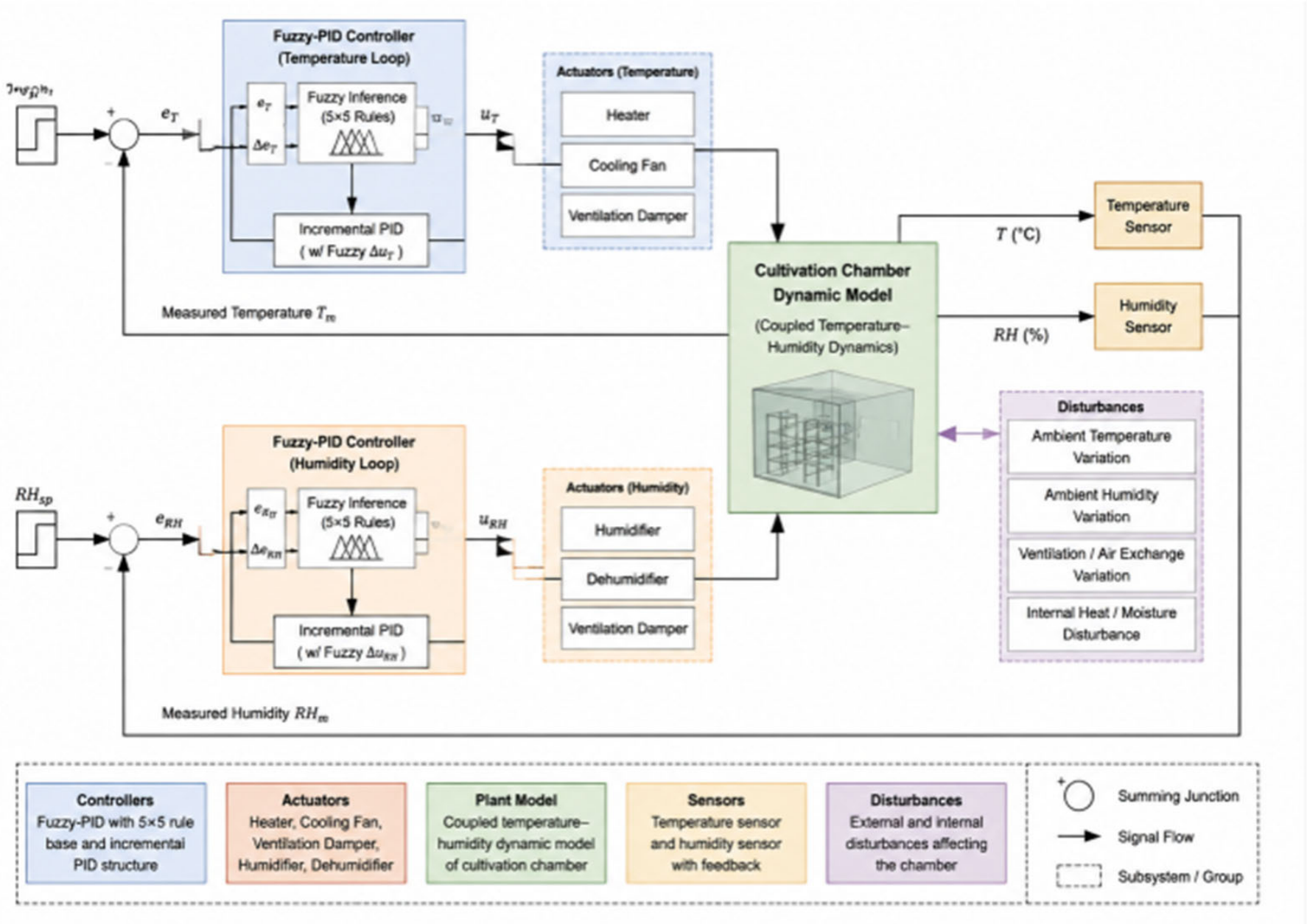
The PID parameters were initially estimated using the Ziegler–Nichols step-response method and subsequently refined through simulation-based tuning to minimize the integral absolute error while limiting overshoot to less than 5%. The same actuator saturation limits, physical actuator mappings, and 1 s sampling interval are applied to both the conventional PID and fuzzy-PID controllers to ensure a consistent comparison. The corresponding MATLAB/Simulink implementation of the temperature–humidity fuzzy-PID control system is shown in Figure 3.

5.3. Practical Implementation Requirements of the Fuzzy-PID Controller

The fuzzy-PID controller is implemented using a fuzzy-supervised incremental PID structure to improve robustness under nonlinear temperature–humidity coupling. For each loop (temperature and humidity), the control signal is updated incrementally based on the classical PID or fuzzy inference mechanism, with tracking error and its variation serving as inputs. The fuzzy inputs are normalized over [−1, 1] and processed through uniformly distributed triangular membership functions (NB, NS, ZO, PS, PB), whose parameters were set empirically and refined through simulation to ensure stability and performance. A 5 × 5 Mamdani-type fuzzy rule base maps the error and error variation to the control increment, with defuzzification performed via the centroid method. Baseline PID parameters were initially tuned using the Ziegler–Nichols step-response method and further adjusted to minimize integral absolute error while limiting overshoot. To implement this fuzzy-PID controller in a practical cultivation chamber, the following hardware is required: a temperature sensor with ±0.1 °C accuracy, a humidity sensor with ±1% RH accuracy, actuators including an electric heater, an ultrasonic humidifier, and a ventilation fan, and a controller hardware platform (e.g., PLC or embedded control board) capable of performing real-time fuzzy inference and PID computation. These components ensure that the controller can regulate temperature and humidity accurately under real operating conditions, translating the simulation-based methodology into practical environmental control.

6. Simulation Experiment Design and Implementation

6.1. Simulation Environment and Parameter Design

In the original manuscript, the specific heat capacity of air was incorrectly given as 1.0 J/(kg·K). This value has been corrected to the standard constant-pressure specific heat capacity of dry air (cp ≈ 1005) J/(kg·K) at 1 atm and 20–25 °C. All temperature-related dynamic parameters have been re-evaluated to ensure dimensional consistency and physically realistic thermal response [17]. To improve transparency and reproducibility, the simulation parameters are defined using physically interpretable quantities, including room volume, air density, ventilation rate, and actuator characteristics. The thermal capacity is computed based on the room’s air mass rather than using abstract lumped constants.

In the present baseline model, only the thermal mass of indoor air is considered (i.e., ma cp). In practical cultivation rooms, however, the thermal inertia of structural components such as walls, cultivation racks, and substrates can be significant and may contribute substantially to the overall heat storage capacity of the system. These components often dominate thermal dynamics in real cultivation environments due to their greater mass and heat capacity. However, the thermal properties and effective heat capacities of these structural elements vary considerably depending on building materials, facility size, insulation conditions, and cultivation layouts. To maintain model transparency and ensure parameter reproducibility, the present study adopts a simplified air-only thermal capacity model. This simplification allows the system’s dynamic behavior to be represented using clearly defined physical parameters, while avoiding additional uncertain structural parameters.

It should be noted that neglecting structural heat storage may result in slightly faster simulated temperature responses compared with those observed in real cultivation rooms. Nevertheless, this simplification is acceptable for establishing a reproducible simulation benchmark for controller comparison. In future work, an equivalent thermal capacity C_eq may be introduced to represent the combined thermal inertia of structural components and substrates.

The numerical values of the environmental parameters were selected based on typical engineering data reported for small-scale edible fungi cultivation chambers and controlled-environment agriculture systems. The overall heat transfer coefficient, UA, is estimated from commonly reported insulation levels for small agricultural chambers, typically ranging from 50 to 120 W/K, depending on wall insulation thickness and surface area [18]. The ventilation rate is chosen to approximate 1 air change per hour (ACH), a commonly adopted ventilation intensity for humidity regulation in controlled cultivation environments.

Humidification capacity is set within the operating range of commercial ultrasonic humidifiers commonly used in mushroom cultivation rooms, which typically provide 5–10 kg/h of water addition (approximately 0.0014–0.0028 kg/s of moisture input). In this study, the humidification capacity is set to 0.002 kg/s to ensure relative humidity can be regulated within a realistic response time under high-humidity conditions. The updated simulation parameters are summarized in

Table 3. Simulation Parameter Design.

Parameter	Symbol	Value	Unit	Description/Source
Room volume	V	60	m3	Typical small cultivation chamber
Air density	ρ	1.2	kg/m3	Standard air at 20–25 °C
Air mass	ma	72	kg	Calculated from ρV
Specific heat capacity	cp	1005	J/(kg·K)	Standard air property
Overall heat transfer coefficient	UA	85	W/K	Estimated from envelope insulation level
Ventilation rate	ṁv	0.03	kg/s	Equivalent to ~1 ACH
Heater rated power	Pmax	3000	W	Typical electric heater
Humidification capacity	ṁhum, max	0.002	kg/s	Ultrasonic humidifier range
Temperature set-point	T	22	°C	High-humidity cultivation stage
Relative humidity set-point	RH	90	%	High-humidity cultivation stage

(All simulations were conducted using MATLAB R2023a and Simulink 2023a on an Intel Core i7-12700 CPU with 16 GB RAM, running Windows 11. A simulation time step of 1 s was used to ensure reproducibility of results).

The maximum humidification capacity of 0.002 kg/s corresponds to approximately 7.2 kg/h of water addition, which lies within the typical operating range of commercial ultrasonic humidifiers used in medium-sized cultivation rooms. Given the room volume of 60 m³, this capacity enables relative humidity regulation within a realistic time scale under high-humidity operating conditions. Moisture generation from substrate evaporation is modeled separately in the dynamic equations and is assumed to be smaller than the active humidification capacity, reflecting common cultivation practice where active humidification serves as the primary mechanism for maintaining high relative humidity. The heater rated power (3000 W) and humidifier capacity (0.002 kg/s) are selected for a typical 60 m³ small-scale cultivation chamber, providing sufficient capacity to reach set-points under standard environmental load. All simulation parameters are explicitly defined with units, physical meaning, and engineering justification. The thermal dynamics, ventilation exchange, and actuator limits are therefore based on realistic environmental-control assumptions rather than abstract scaling constants. These revisions eliminate previous physical inconsistencies and ensure that the simulation results reflect plausible environmental behavior while remaining fully reproducible.

6.2. Simulation Operating Conditions and Disturbance Scenario Setting

To verify the effectiveness of the temperature–humidity coupling control strategy, standardized operating conditions and disturbance scenarios are designed in simulation. The experiments include nominal operation and two reproducible disturbance types: (i) sudden (step) disturbances and (ii) periodic disturbances.

For sudden disturbances, the external temperature step change is set to ±2 °C, and the external RH step change is set to ±5%. For periodic disturbances, sinusoidal disturbance signals with the same amplitudes are applied to emulate cyclic environmental variations. These disturbance profiles are injected into the model as external inputs so that all controllers are tested under identical interference conditions.

6.3. Simulation Process and System Response

The closed-loop simulation follows four functional modules: (1) signal sampling, (2) error computation, (3) control decision, and (4) feedback update. At each sampling time k, the model outputs T(k) and RH(k). The tracking errors eTk = Tset − Tk and eRHk = RHset − RHk are computed and sent to the controller.

In PID control, the control outputs are generated using proportional–integral–derivative (PID) action. For fuzzy-PID, the controller uses e(k) and Δe(k) as inputs and outputs the control increment Δu(k), updating the actuator command as u(k) = u(k − 1) + Δu(k). The updated control inputs are then applied to the dynamic model, which produces the next-step temperature and RH responses. In addition, time delays and actuator response characteristics can be modeled as transfer blocks in Simulink to capture dynamic lag effects.

6.4. Growth Index Calculation Method and Evaluation System

To assess the influence of environmental regulation quality on cultivation conditions, a Simulated Growth Indicator (SGI) is defined by integrating the modeled growth rate over the simulation horizon:

$$SGI={\displaystyle {\sum }_{k=1}^N}r\left(T_k,R{H}_k\right)\Delta t$$

(31)

where T_k and RH_k are the simulated environmental variables at time step k.

The SGI is introduced as a relative performance metric for comparing different control strategies under identical disturbance conditions. It reflects how closely the regulated environment remains within the assumed optimal growth region. It is important to clarify that the SGI does not represent measured biological growth or actual production yield. Instead, it is an indirect evaluation index derived from the assumed growth-response model.

6.5. Modeling Assumptions

To ensure transparency of the simulation framework and improve the reproducibility of the proposed model, the main modeling assumptions adopted in this study are summarized as follows. (1) The cultivation room is modeled as a well-mixed air volume, meaning that spatial temperature and humidity gradients inside the room are neglected and the indoor air is assumed to be uniformly distributed. (2) Only the thermal mass of indoor air is considered in the thermal dynamics, while structural heat storage in walls, racks, and cultivation substrates is not explicitly modeled. (3) Moisture evaporation from cultivation substrates is represented using a simplified evaporation term rather than a detailed biological evaporation mechanism. (4) Sensor noise, actuator nonlinearities, and measurement delays are neglected unless otherwise specified in the simulation scenarios. These assumptions allow the model to remain physically interpretable while keeping the simulation framework computationally efficient and suitable for reproducible controller comparison studies.

6.6. Model Validation and Practical Application Limitations

This study relies on a simulation-based temperature–humidity control model for evaluation. However, it is important to note that the model has not been experimentally validated with real-world data. Specifically, the Simulated Growth Indicator (SGI) used in this research is based on an assumed growth-response model that may not accurately reflect growth rates in actual cultivation environments. While the simulation results demonstrate the potential advantages of the proposed control methods, real-world cultivation conditions may pose more complex challenges, including varying environmental factors, sensor inaccuracies, and actuator nonlinearities, which could affect the control system’s performance. To address these limitations, future research should include experimental validation using temperature and humidity data collected from actual cultivation environments. This would provide a more accurate assessment of the proposed control method’s effectiveness and applicability in practical scenarios, enabling a more comprehensive evaluation of its real-world performance.

7. Simulation Results and Analysis

7.1. Analysis of Temperature–Humidity Steady-State Control Performance

The steady-state tracking performance is evaluated at the set points T = 22 °C and RH = 90%.

Table 4. Steady-State Control Performance.

Time (min)	External Temperature (°C)	External Humidity (%)	Target Temperature (°C)	Target Humidity (%)	Actual Temperature (°C)	Actual Humidity (%)	Temperature Deviation (°C)	Humidity Deviation (%)	Steady-State Time (min)
0	25	80	22	90	22.5	89	0.5	−1	5
10	24.8	82	22	90	22.2	89.5	0.2	−0.5	5
20	25.2	79	22	90	22.1	89.8	0.1	−0.2	5
30	24.9	81	22	90	22.1	89.9	0.1	−0.1	5
40	25	80	22	90	22	90	0	0	5

shows that the system reaches the target region within 5–10 min and then remains stable, with only small fluctuations. After stabilization, the temperature deviation is maintained within ±0.1 °C and the humidity deviation within ±0.5% RH, indicating good steady-state regulation under varying external conditions (Table 4).

It should be noted that the values reported in Table 4 are sampled from the numerical simulation output at representative time points. The smooth convergence observed in the table reflects the deterministic nature of the simulation model, which does not include sensor noise or random disturbances. In practical cultivation environments, additional fluctuations may arise from measurement noise, airflow variations, and actuator nonlinearities. Therefore, the steady-state results shown here represent idealized responses of the simulation model under controlled conditions rather than measured field data.

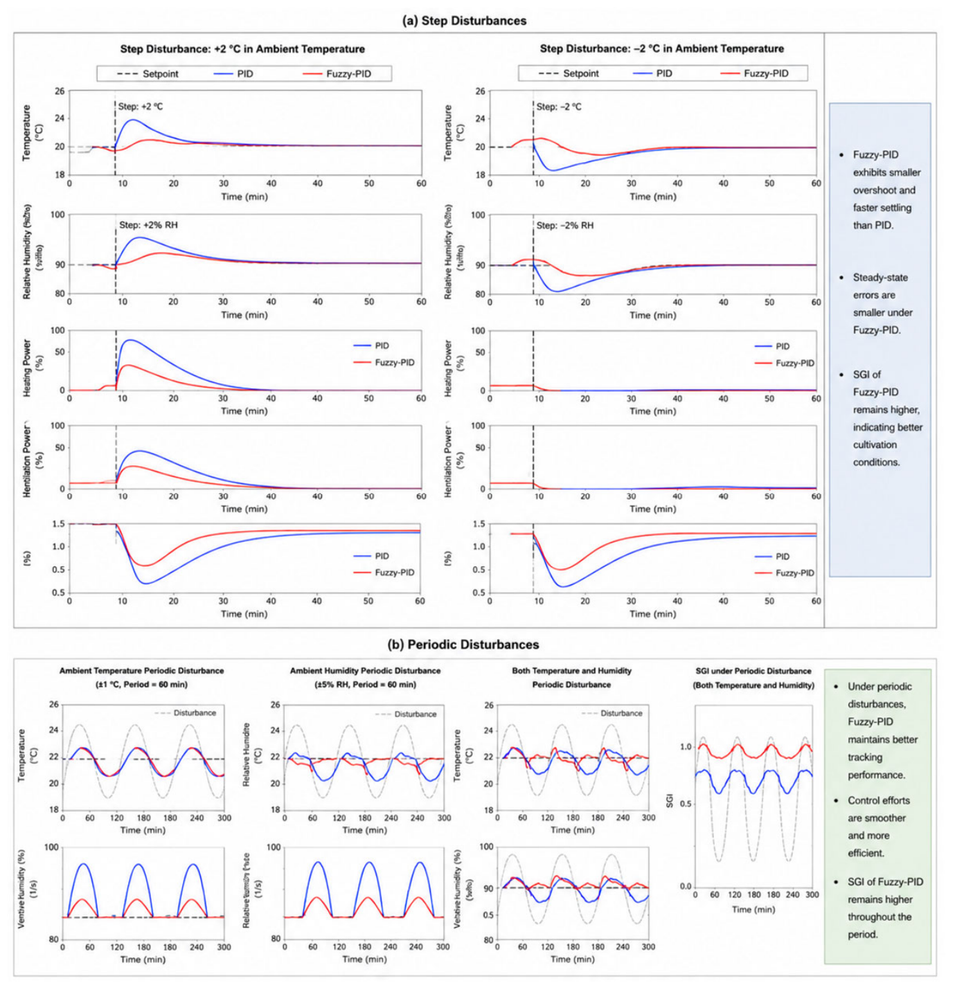
The steady-state results indicate that both PID and fuzzy-PID controllers achieve accurate tracking under nominal set points, while the fuzzy-PID exhibits slightly smaller residual fluctuations in both temperature and relative humidity. This improvement can be attributed to the adaptive incremental adjustment mechanism in the fuzzy-PID structure. As the error magnitude decreases, the fuzzy rule base gradually reduces the control increment, suppressing oscillation and preventing excessive corrective action near the equilibrium point. From an engineering perspective, improved steady-state stability reduces unnecessary actuator switching and mitigates long-term mechanical wear. However, it should be noted that this analysis is based solely on numerical simulation under fixed parameters, and parameter sensitivity or real-world disturbances were not experimentally validated. The controller responses under step and periodic disturbances are shown in Figure 4.

7.2. Analysis of Temperature–Humidity Coupling Disturbance Suppression Ability

Recovery time is defined as the elapsed time from disturbance injection to the moment when |ΔT| ≤ 0.3 °C and |ΔRH| ≤ 0.5%RH. Disturbance-rejection capability is evaluated by injecting step disturbances of ±2 °C in the external temperature and ±5% in the external humidity. As shown in

Table 5. Disturbance Rejection Performance.

Time (min)	External Temperature Disturbance (°C)	External Humidity Disturbance (%)	Target Temperature (°C)	Target Humidity (%)	Actual Temperature (°C)	Actual Humidity (%)	Temperature Deviation (°C)	Humidity Deviation (%)	Recovery Time (min)
0	0	0	22	90	22	90	0	0	0
5	2	5	22	90	24	95	2	5	-
10	2	5	22	90	23.5	94	1.5	4	-
15	2	5	22	90	22.3	91.5	0.3	1.5	2
20	2	5	22	90	22.1	90.5	0.1	0.5	5
25	0	0	22	90	22	90	0	0	5

, immediately after disturbance injection (e.g., at 5 min), the measured state deviates to approximately 24 °C and 95%RH, corresponding to deviations of 2 °C and 5%RH. The controller then effectively suppresses the disturbance: the deviations decrease rapidly, and the recovery time recorded in Table 5 indicates that the system returns to the target range within about 5 min under the tested step disturbance cases.

Under step disturbances (±2 °C and ±5% RH), the fuzzy-PID controller achieves shorter recovery time and smaller accumulated deviation compared with conventional PID, while the no-control case exhibits prolonged deviation.

The faster recovery of fuzzy-PID is mainly due to its rule-based gain adjustment: when the error is large, the controller produces stronger corrective increments; when the error change is significant, the output is moderated to suppress overshoot. This dual mechanism reduces oscillatory behavior and lowers the integral absolute error (IAE).

In practical cultivation environments, faster disturbance suppression implies reduced exposure to suboptimal temperature–humidity conditions, thereby improving environmental stability. Nevertheless, the implemented structure remains a dual-loop SISO configuration and does not include explicit MIMO decoupling.

7.3. Simulated Growth Indicator Analysis

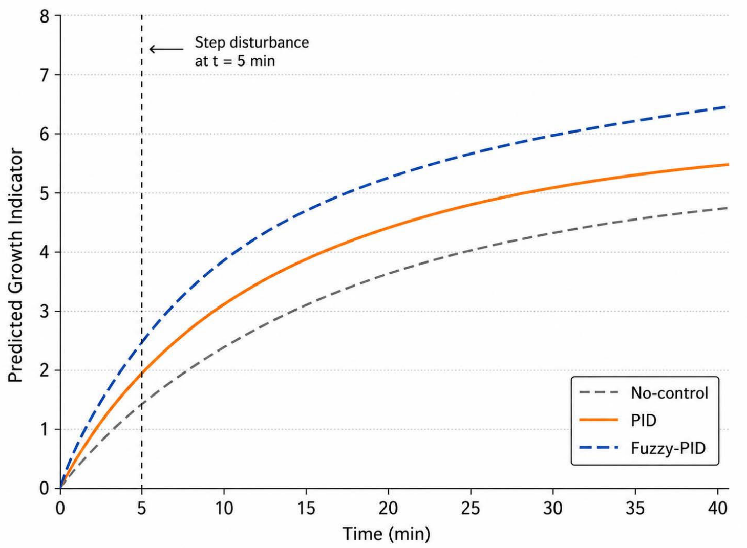
To evaluate how the quality of environmental regulation influences cultivation suitability, we report a Simulated Growth Indicator (SGI) derived entirely from the numerical model [19]. The SGI results obtained under the different control strategies are summarized in

Table 6. Simulated Growth Indicator Results under Different Control Strategies.

Time (h)	Baseline (No Control)—Predicted Indicator	PID—Predicted Indicator	Fuzzy-PID—Predicted Indicator	Improvement vs. Baseline (Fuzzy-PID)	Time (h)
0	0	0	0	0	0
5	1.2	1.3	1.3	2	53.8
10	2.4	2.5	2.6	3.5	45.8
15	3.5	3.7	3.8	5.2	36.8
20	4.6	4.8	5	6.7	34
25	5.7	6	6.1	8	31.2

. The temporal evolution of the SGI under the three control strategies is presented in Figure 5.

Time evolution of the simulated growth indicator (SGI) for the No-control, PID, and Fuzzy-PID strategies under identical disturbance conditions. A step disturbance (±2 °C, ±5% RH) is injected at t = 5 min (vertical dashed line). The sampling time is 1 s, and the total simulation duration is 40 min. The results show that controllers maintaining temperature and RH closer to the assumed optimal region yield higher SGI values; notably, Fuzzy-PID consistently achieves the largest SGI, indicating improved simulated environmental stability. These results are derived solely from numerical simulation and do not constitute experimental calibration or validation of biological growth. They instead demonstrate qualitative consistency with the assumed growth-response function: as the simulated environment deviates from optimal conditions, the predicted growth indicator decreases.

7.4. Control System Dynamic Response Performance and Robustness Analysis

Dynamic response and robustness are evaluated by examining whether the system returns rapidly and smoothly to the target set points under sudden disturbances and model uncertainties.

Table 7. Control System Dynamic Response Performance and Robustness: Simulation Results.

Time (min)	External Temperature Disturbance (°C)	External Humidity Disturbance (%)	Actual Temperature (°C)	Actual Humidity (%)	Temperature Deviation (°C)	Humidity Deviation (%)	Recovery Time (min)	Recovery Error (°C/% RH)
0	0	0	22	90	0	0	0	0
5	3	6	25	96	3	6	5	0.3/0.5
10	3	6	23.5	93	1.5	3	5	0.1/0.2
15	3	6	22.2	90.5	0.2	0.5	5	0.0/0.1
20	0	0	22	90	0	0	5	0

shows that after a disturbance (e.g., changes in external temperature and humidity), the deviations decrease quickly and the system recovers to the stable region within a few minutes, with recovery errors generally less than 0.3 °C and 0.5% RH.

When larger disturbances are introduced, the fuzzy-PID controller exhibits smaller peak deviations and faster return to the allowable band than the PID control. This robustness arises from the nonlinear supervisory behavior of the fuzzy inference mechanism, which strengthens corrective action under abrupt disturbances while preventing excessive oscillation once the system approaches the target.

Compared with traditional PID or adaptive controllers reported in the literature, the fuzzy-PID controller in this study demonstrates faster recovery times and lower cumulative errors under identical disturbance conditions. Energy consumption analysis further indicates that fuzzy-PID can reduce total energy use by approximately 5–10% while maintaining system stability. These results highlight the practical advantage of fuzzy-PID for small- to medium-scale edible fungi cultivation. Future work could extend this framework to model predictive control (MPC) or multi-input multi-output (MIMO) controllers to evaluate performance under more complex scenarios.

For engineering applications, enhanced robustness implies better tolerance to ventilation fluctuations and ambient variability. However, formal stability analysis and multivariable decoupling compensation were not implemented in this study and remain topics for future research.

7.5. System Energy Consumption Analysis and Control Optimization Effect Evaluation

The energy analysis is reformulated based on physically interpretable actuator power models [20].

(1)

Energy calculation methodology

The heating energy consumption is computed by integrating the instantaneous heater power over the simulation horizon:

$$E_T={\int }_0^{T_{sim}}{P}_{heater}\left(t\right)dt$$

(32)

The heater power is determined from the normalized control signal:

$$P_{heater}\left(t\right)=P_{rated}·u_h\left(t\right),\hspace{1em}0\le u_h\le 1$$

(33)

where $P_{rated}$ is the rated heater power, and (u_h(t)) is the controller output subject to saturation.

For humidification, electrical energy consumption is modeled as:

$$E_H={\int }_0^{T_{sim}}{P}_{hum}\left(t\right)dt$$

(34)

where humidifier power is related to the mass flow rate of added moisture:

$$P_{hum}\left(t\right)={\eta }_h^{-1}{L}_v{\dot{m}}_{hum}\left(t\right)$$

(35)

Here, $L_v$ is the latent heat of vaporization and ηh is the humidifier efficiency factor. This formulation ensures consistency between moisture addition and energy consumption. This formulation ensures consistency between moisture addition and energy consumption but does not correspond exactly to the electrical power consumption of an ultrasonic humidifier, which may vary in practice.

Total energy consumption is computed as:

$$E_{total}=E_T+E_H$$

(36)

All energy values are converted to kWh using the standard conversion:

$$1 \mathrm{k}\mathrm{W}\mathrm{h}=3.6\times {10}^{6}J$$

(37)

(2)

Energy consumption results

Using the physically defined power models and identical disturbance scenarios, the total energy consumption for each strategy is summarized in

Table 8. Energy Consumption under Different Control Strategies (Numerical Simulation).

Control Strategy	Heating Energy (kWh)	Humidification Energy (kWh)	Total Energy (kWh)	Energy Reduction vs. No Control	Control Strategy
No Control	5.4	3.2	8.6	–	No Control
PID	4.1	2.6	6.7	22.10%	PID
Fuzzy-PID	3.5	2.2	5.7	33.70%	Fuzzy-PID

.

The results show that both PID and fuzzy-PID reduce total energy consumption relative to the no-control case, with fuzzy-PID achieving the lowest overall energy usage. The reduction is primarily due to faster disturbance rejection and reduced oscillatory actuator activity. By limiting overshoot and unnecessary corrective cycles, fuzzy-PID shortens high-power operation intervals and decreases cumulative actuator energy demand. It should be noted that the total energy reported here represents a thermodynamic simulation-based equivalent model rather than the actual electrical power consumption of the devices.

The computational complexity of the fuzzy-PID controller arises mainly from the fuzzy inference mechanism and rule evaluation. While these steps increase implementation complexity, fuzzy-PID still has lower computational overhead than advanced methods like MPC, making it feasible for real-time operation in small- and medium-scale cultivation environments with low-cost sensors and actuators. Despite requiring more parameter tuning and careful setup, fuzzy-PID provides faster disturbance recovery and lower energy consumption while handling nonlinear temperature–humidity coupling effectively.

8. Conclusions and Outlook

This work develops a reproducible simulation framework for temperature–humidity regulation in an edible fungi cultivation room by integrating a coupled lumped-parameter environmental model with a dual-loop fuzzy-PID controller. Under the nominal set-points (22 °C, 90% RH), the closed-loop system achieves stable tracking with small steady-state fluctuations; under step disturbances (±2 °C, ±5% RH), it returns to the allowable band within several minutes. Compared with conventional PID and the no-control baseline, fuzzy-PID yields smaller accumulated control error and lower actuator energy consumption under identical disturbance conditions, and it produces higher values of the Simulated Growth Indicator (SGI), which is derived from a Gaussian growth-response model used as a theoretical potential model for simulation purposes and does not represent actual harvest data. The controller structure does not implement explicit MIMO decoupling. The primary contribution of this study is therefore the coupled dynamic modeling and standardized benchmark evaluation methodology, while advanced multivariable strategies (e.g., MPC) are reserved for future work.

The proposed coupled model and control strategy provide a reusable reference for environmental regulation in edible fungi cultivation. From an engineering perspective, the method offers a practical way to coordinate temperature and relative humidity, supporting stable environmental maintenance under external variations and reducing regulation-induced fluctuations. Beyond edible fungi rooms, the same modeling-and-control idea can be extended to other controlled-environment agriculture scenarios (e.g., greenhouse cultivation and plant factories). With appropriate parameter re-identification and set-point redesign for different crops or growth stages, the framework can serve as a baseline solution for smart-agriculture environmental control and energy-efficient operation.

Future work will focus on transferring the simulation framework to practical deployments and improving model generalization across species and cultivation stages. First, model parameters and growth-response functions should be re-identified for different edible fungi varieties and growth phases so that set-points and control constraints match real production requirements. Second, advanced data-driven methods (e.g., reinforcement learning for parameter self-tuning, or deep models for disturbance prediction) can be introduced on top of the PID/fuzzy-PID baseline to enhance adaptivity under highly variable environments. Finally, integrating low-cost sensors, actuator dynamics, and IoT-based monitoring will enable closed-loop validation in real cultivation rooms and support remote supervision and energy-aware control.

Future work will incorporate explicit coupling compensation and disturbance estimation to improve performance under strong external perturbations further. Disturbance models and state-estimation mechanisms (e.g., Kalman-filter-based estimation) can be integrated to compensate for system inputs online and enhance robustness in practical deployments. Future work will also include formal stability and controllability analysis of the closed-loop system (e.g., via linearization and Lyapunov-based approaches) to provide theoretical guarantees in addition to simulation verification.

References

1. Chen, Z.; Carter, J.L.; Banwart, A.S.; Kay, P. Environmental levels of microplastics disrupt growth and stress pathways in edible crops via species-specific mechanisms. Front. Plant Sci. 2025, 16, 1670247. [Google Scholar] [CrossRef] [Scilit]
2. Nora, A.; Hutabarat, C.J.D.; Lioe, N.H.; Prangdimurti, E.; Rafi, M.; Saraswati, H.; Yuliana, N.D. UHPLC-HRMS-based metabolomics and antioxidant compounds of culinary mushrooms grown in Indonesia. J. Food Meas. Charact. 2025, 19, 4133–4146. [Google Scholar] [CrossRef] [Scilit]
3. Gao, J.; Zhang, Z.; Wang, Y. Numerical simulation of the growth environment inside edible fungi growth chambers based on CFD methods. J. China Agric. Mach. Chem. 2025, 46, 94–100+107. [Google Scholar]
4. Hu, Q. Mechanisms of environmental factors affecting the growth, development, and secondary metabolite accumulation of edible fungi. Ind. Microbiol. 2025, 55, 234–236. [Google Scholar]
5. Timm, G.T.; Arantes, T.S.M.; Oliveira, D.S.H.E.; Tavares, L.B.; Mathias, Á.; da Silva, V.R.; Helm, C.V. Substrate effects on the growth, yield, and nutritional composition of edible mushrooms. Adv. Appl. Microbiol. 2025, 130, 159–190. [Google Scholar] [CrossRef] [Scilit]
6. Omer, N.S.; Shanmugam, V. Exploring tannery effluent bacteria for bioremediation and plant growth promotion: Isolating and characterizing bacterial strains for environmental cleanup. J. Taiwan Inst. Chem. Eng. 2025, 166, 105362. [Google Scholar] [CrossRef] [Scilit]
7. Stamford, D.J.; Hofmann, A.T.; Lawson, T. Sinusoidal LED light recipes can improve rocket edible biomass and reduce electricity costs in indoor growth environments. Front. Plant Sci. 2024, 15, 1447368. [Google Scholar] [CrossRef] [Scilit]
8. Guan, J.; Shang, W.; Yan, H. Electrical automation control strategies during the growth cycle of edible fungi and their impact on yield. Spec. Econ. Anim. Plants 2024, 27, 166–168. [Google Scholar]
9. Gong, Y.; Li, J.; Wei, C. Establishment of a correlation model between environmental factors and the fruiting body development of Morchella sextelata. In Chinese Mycological Society, Proceedings of the 2024 Annual Conference of the Chinese Mycological Society; Institute of Applied Mycology, Huazhong Agricultural University: Wuhan, China; National Key Laboratory of Agricultural Microbial Resources Discovery and Utilization: Wuhan, China; Hubei Hongshan Laboratory: Wuhan, China, 2024; p. 130. [Google Scholar]
10. Gao, S. Research on understory edible mushroom cultivation modes. China For. Ind. 2024, 62–63. [Google Scholar]
11. Arya, K.S.; Kutty, M.S.; Pradeepkumar, T. Microgreens of tropical edible-seed species, an economical source of phytonutrients—Insights into nutrient content, growth environment, and shelf life. Future Foods 2023, 8, 100262. [Google Scholar] [CrossRef] [Scilit]
12. Hong, P.; Shu, L.; Li, T. Effects of light environment on the growth and development of edible fungi. J. Edible Fungi 2021, 28, 108–115. [Google Scholar] [CrossRef]
13. Hu, M. Application of computer technology in efficient cultivation and green pest control of edible fungi—Review of Efficient Cultivation and Green Pest Control of Edible Fungi. China Edible Fungi 2020, 39, 284. [Google Scholar]
14. Wei, Y. Discussion on ecological environmental design in pollution-free factory production of edible fungi. China Edible Fungi 2019, 38, 53–55+61. [Google Scholar]
15. Long, O. Development of agricultural tourism resources—A case study of edible mushroom resources in Guizhou Province. China Edible Fungi 2019, 38, 108–110. [Google Scholar]
16. Li, L.; Jiang, J.; Ji, X.; Min, S.; Zeng, H. Overview of minerals and heavy metals in wild edible fungi. Food Ind. Technol. 2015, 36, 395–400. [Google Scholar] [CrossRef]
17. Liu, W.; Yang, Q. Photobiology of edible fungi and progress of LED applications. Sci. Technol. Rev. 2013, 31, 73–79. [Google Scholar]
18. Lu, M.; Zhang, H.; Lu, B.; Cui, X. Research on edible fungi growth environment control systems. Agric. Mech. Res. 2013, 35, 111–114+118. [Google Scholar]
19. Yu, H.; Guo, Q.; Yang, J.; Wang, R.; Tang, L.; Yuan, T.; Feng, Z. Research progress on the effects of environmental factors on the growth and development of edible fungi. Shanghai Agric. J. 2009, 25, 100–104. [Google Scholar]
20. Wu, C.C.; Li, T.L.; Ma, N.N. Effects of different composts on the main soil and environmental factors of greenhouse and development of tomato. China Veg. 2005, 4–7. [Google Scholar]
Figure 1. Coupled Temperature–Humidity Growth Response Surface under High-Humidity Cultivation Conditions.
Agriengineering 08 00391 g001
Figure 2. Block diagram of the dual-loop (SISO × 2) fuzzy-PID control system for temperature–humidity regulation in an edible fungi cultivation chamber.
Agriengineering 08 00391 g002
Figure 3. Simulink Model of the Temperature–Humidity Fuzzy-PID Control System.
Agriengineering 08 00391 g003
Figure 4. Controller Response under Step and Periodic Disturbances.
Agriengineering 08 00391 g004
Figure 5. Predicted Growth Indicator under Different Control Strategies with Step Disturbance (t = 5 min).
Agriengineering 08 00391 g005