An Archard-Informed Gaussian Process Residual-Learning Surrogate Model for DEM-Based Wear Prediction of Soil-Engaging Components

Abstract

Wear prediction for agricultural soil-engaging components is computationally demanding when discrete element method (DEM) simulations are repeatedly used for design evaluation and operating-parameter screening. In this study, an Archard-inspired Gaussian process regression (GPR) residual-learning surrogate was developed for rapid prediction of the total wear volume calculated by EDEM for a ploughshare. The physical prior was a monotonic operational-parameter proxy motivated by the load and sliding trends in Archard theory, which did not directly use DEM-derived normal force, sliding distance, or frictional work. A soil–ploughshare interaction model was used to generate 100 full-factorial samples with tillage depth, tillage speed, and penetration angle as inputs. The Archard-inspired prior, cubic polynomial Ridge regression, standard GPR, and prior-guided residual GPR were evaluated by cross-validation, repeated random splits, and boundary-level extrapolation tests. Across 30 repeated 90%/10% splits, standard and Archard-inspired GPR achieved mean R² values of 0.9927 ± 0.0014 and 0.9908 ± 0.0021, respectively. In the 200 mm tillage-depth extrapolation test, the latter performed best, with R² = 0.9752, RMSE = 0.000252 mm³, and MAPE = 2.68%; however, the former was more accurate in the tillage-speed and penetration-angle extrapolation tests, and the 48% interval coverage of the prior-guided model in the penetration-angle test indicated overconfidence when the prior was biassed. These results show a conditional, rather than universal, benefit of the Archard-inspired prior: it improved extrapolation plausibility for the load-dominated tillage-depth case but did not improve all boundary predictions. The surrogate predicts EDEM-simulated wear, and its engineering validity depends on DEM calibration, the selected wear coefficient, and future soil-bin or field validation.

1. Introduction

Soil-engaging components are subjected to repeated cutting, compression, sliding, and impact by soil particles, sand, gravel, and crop residues. Abrasive wear changes tool geometry, reduces penetration and tillage-depth stability, and increases maintenance cost and downtime, and previous reviews have shown that wear is affected by soil particle size and moisture, operating depth and speed, component material, and geometry [1]. A reliable relationship between operating parameters and wear is therefore useful for wear-resistant design and operating-parameter screening.

Field, soil-bin, and bench wear tests provide direct evidence under physical operating conditions, but they are time-consuming, expensive, and difficult to control at the local contact scale, whereas the discrete element method (DEM) provides particle-scale information on force, motion, sliding, contact frequency, and energy dissipation and has been widely used to study soil cutting, tillage resistance, soil disturbance, and soil–tool interaction [2,3,4,5,6]. When combined with a wear law, the DEM can also provide a spatial and quantitative estimate of simulated surface wear; however, repeated DEM simulations across many operating conditions remain computationally expensive.

The classical Archard model relates wear volume to normal load and relative sliding distance, with material hardness and a wear coefficient acting as scaling terms [7]. Archard-type formulations have been combined with the DEM and other numerical methods to simulate wear of tillage and soil-engaging tools [8,9,10,11]; nevertheless, an EDEM wear output remains model-dependent: it is affected by particle and contact parameters, boundary conditions, the selected wear coefficient, and the calibration quality of the DEM model. A surrogate trained on such data predicts the simulation response and should not be interpreted as a direct predictor of field wear life without experimental calibration.

Surrogate models are commonly used for expensive computer experiments [12,13]. Polynomial response surfaces are simple and interpretable, and Ridge regularization can reduce instability caused by correlated high-order terms [14,15]. GPR is particularly suitable for low-dimensional, small-sample nonlinear regression because it provides both a predictive mean and a predictive variance [16,17,18,19]; however, a purely data-driven GPR may revert toward its mean outside the training domain, whereas a misspecified physical prior may introduce systematic bias.

Physics-informed and hybrid machine learning methods combine data with scientific knowledge through features, loss functions, model structures, or physical-model residuals [20,21,22], and similar ideas have been explored in wear prediction [23,24]. In the present problem, direct Archard variables such as accumulated normal force and sliding distance were not used as model inputs; instead, a constrained operational-parameter function was constructed from tillage depth, speed, and penetration angle to represent a simplified wear trend. It is therefore more accurately described as Archard-inspired rather than as a complete implementation of the Archard mechanism.

The methodological contribution of this study is domain-specific rather than a new general GPR formulation, and consists of the following: (i) a monotonic Archard-inspired mean function in the operating-parameter space; (ii) GPR residual correction under small-sample conditions; (iii) an ablation comparison among prior-only, zero-prior/data-only GPR, and prior-guided residual GPR; (iv) separate interpolation and boundary-level extrapolation tests that identify both the benefit and the failure modes of the prior. We ask not whether the physical prior is universally superior, but under which operating-variable extrapolations it improves prediction plausibility.

Accordingly, EDEM-simulated total wear volume is modelled as a function of tillage depth, tillage speed, and penetration angle, and the models are evaluated by cross-validation, repeated random splits, boundary extrapolation, and uncertainty calibration. The engineering scope and the limitations caused by fixed DEM settings, a fixed wear coefficient, and the absence of independent experimental wear measurements are explicitly discussed.

2. Materials and Methods

2.1. Research Object and Workflow

This study focuses on the wear volume of agricultural soil-engaging components during soil operation. Wear data under different operation-parameter combinations are obtained from EDEM-based DEM simulations, and an Archard-informed GPR model is established. The input variables are tillage depth d, tillage speed v, and penetration angle α, and the output variable is the total wear volume V calculated by EDEM. Because the dataset contains only 100 samples, the input dimension is low, and the samples come from computationally expensive simulations. This study does not use deep neural networks that typically require large-scale data; instead, GPR is selected as the main model because it is suitable for small-sample nonlinear regression and can provide prediction uncertainty.

The workflow comprises four stages: first, an EDEM soil–ploughshare model is used to generate total wear volume under a 5 × 5 × 4 full-factorial set of tillage depth, tillage speed, and penetration angle; second, all preprocessing and model fitting are performed within the training data of each validation split; third, four models are compared—an Archard-inspired prior-only model (M₁), cubic polynomial Ridge regression (M₂), a zero-prior/data-only GPR (M₃), and an Archard-inspired prior plus GPR residual correction (M₄); fourth, performance is assessed using cross-validation, repeated random splits, three boundary-level extrapolation tests, and prediction interval calibration. The comparison between M₁, M₃, and M₄ serves as an ablation analysis of the prior and residual components. The technical flowchart of the present work is presented in Figure 1.

2.2. EDEM Simulation Model and Wear-Data Acquisition

2.2.1. Ploughshare Model

The ploughshare geometry is built using three-dimensional modelling software. The model mainly retains the working surface and the key surfaces that directly contact soil, but non-essential structures are simplified to reduce the computational cost, without changing the main geometric features and soil-contact relationship. The simplified ploughshare model and its main dimensions are shown in Figure 2.

2.2.2. Soil Model

The soil medium is represented by single-sphere particles, whose basic physical radius is set to 10 mm. To represent particle-size variability, a radius-based random size distribution is adopted with a scaling factor of 0.95–1.05, meaning that the actual particle radius is uniformly distributed between 9.5 and 10.5 mm. A total of 857,208 particles are generated to ensure a sufficient and representative particle population in the soil-bin model. The discrete soil model is shown in Figure 3.

2.2.3. Material and Contact Parameters

The density, Poisson’s ratio, and shear modulus of the ploughshare and soil, as well as the friction coefficients, restitution coefficients, and cohesion-related parameters both between particles and between particles and the component, are set according to Refs. [25,26]. The specific parameters are listed in

Table 1. Material and contact parameters of soil particles and ploughshare.

Property	Value
Density of steel (kg·m−3)	7865
Shear modulus of steel (Pa)	7.9 × 1010
Poisson’s ratio of steel	0.3
Density of soil (kg·m−3)	2600
Shear modulus of soil (Pa)	5 × 107
Poisson’s ratio of soil	0.3
Coefficient of static friction of soil particles	0.7
Coefficient of static friction of steel–soil	0.5
Coefficient of rolling friction of soil particles	0.225
Coefficient of rolling friction of steel–soil	0.05
Coefficient of restitution of soil particles	0.6
Coefficient of restitution of soil–steel	0.6
Surface energy (J·m−2)	6

.

2.2.4. Contact Model

In DEM simulations, the interaction both between soil particles and between soil particles and the ploughshare surface is described by contact models. Considering that soil particles undergo normal compression, tangential friction, rolling resistance, and a certain degree of cohesion during tillage, the Hertz–Mindlin with JKR model and the Standard Rolling Friction model are used to describe particle–particle and particle–component contact behaviour. This combined model represents particle motion under compression, shear, and friction and is suitable for simulating particle disturbance, soil failure, and ploughshare force variation during ploughshare soil cutting.

2.2.5. Archard Wear Model

Wear volume is calculated based on the classical Archard wear model, which expresses wear volume as a function of normal load and relative sliding distance while considering material hardness:

$$V=K{\displaystyle \frac{F_{n}s}{H}}$$

(1)

where V is wear volume, K is the dimensionless wear coefficient, F_n is the normal contact load, s is the relative sliding distance, and H is material hardness. For particle–geometry contact in DEM simulations, the wear volume can be written as the cumulative contribution of multiple contact events:

$$V=K{\displaystyle \sum _{i=1}^n\frac{F_{N,i} \mathrm{\Delta }{s}_i}{H}}$$

(2)

where $F_{N,i}$ is the normal contact force in the i-th contact event, $\mathrm{\Delta }{s}_i$ is the relative sliding distance in that contact event, and n is the total number of contact events. The Archard wear model in EDEM calculates surface wear by accumulating the contact load and sliding distance between particles and geometry surfaces. In this study, the wear coefficient is set to K = 1 × 10⁻¹⁵ and remains unchanged for all working conditions; this value was used as a numerical scaling value to maintain the simulated wear volume within a suitable computational range, was fixed for all 100 simulations, and was not calibrated against experimentally measured ploughshare mass or volume loss. Therefore, the absolute wear-volume values obtained in this study should be interpreted as model-dependent EDEM outputs for relative comparison among working conditions under the same simulation configuration, rather than as direct estimates of field wear or service life. Experimental calibration of K is required before absolute engineering wear predictions can be made. Therefore, differences in wear among samples mainly arise from changes in contact load, sliding distance, contact frequency, and soil flow state.

2.2.6. Wear-Volume Extraction

Wear is quantified by total wear volume. A statistical region S is first defined to cover the main working surface of the ploughshare, as shown in Figure 4; the EDEM data processing module is then used to output the area A_i of each surface element within region S and the corresponding wear depth h_i; and finally, a Python programme is used to calculate total wear volume by summing the wear volume of all surface elements:

$$V={\displaystyle \sum A_i{h}_i}$$

(3)

where A_i is the area of the i-th surface element and h_i is the wear depth on that element. Each working condition generates an independent EDEM simulation result file. In this study, the total wear volume at an operating distance of 10 m is extracted as the model output, the calculation process of wear volume is illustrated in Figure 5.

2.3. Working-Condition Design and Dataset

Tillage depth, tillage speed, and penetration angle are used as control variables, and their definitions are shown in Figure 6. A full-factorial experimental design is used to construct the simulation conditions; tillage depth, tillage speed, and penetration angle have five, five, and four levels, respectively, resulting in 100 working conditions, as listed in

Table 2. Simulation working conditions.

Factor	Symbol	Level	Unit
Tillage depth	d	100, 125, 150, 175, 200	mm
Tillage speed	v	1.00, 1.25, 1.50, 1.75, 2.00	m/s
Penetration angle	α	15, 30, 45, 60	°

.

A full-factorial design was used because the problem contains only three factors and 100 combinations, making complete coverage computationally feasible. The regular grid also permits transparent boundary-level tests in which an entire factor level is excluded from training, while retaining all combinations of the other two factors. Latin hypercube, Sobol, and adaptive designs can be more efficient for higher-dimensional or larger design spaces, but they do not provide the same direct level-by-level separation for the present extrapolation analysis. The current design was therefore selected for interpretability and systematic boundary evaluation rather than as a claim of globally optimal sampling efficiency. The dataset can be expressed as follows:

$$D={\left\{\left(x_i,V_i\right)\right\}}_{i=1}^N$$

(4)

where $x_i=\left(d_i,v_i,{\alpha }_i\right)$ is the input vector of the i-th working condition, V_i is the corresponding total wear volume, and N = 100. The statistical results show that V ranges from 0.001825 to 0.011278 mm³, with a mean value of 0.005284 mm³ and a standard deviation of 0.002204 mm³. The minimum wear occurs at a tillage depth of 100 mm, a tillage speed of 1.25 m/s, and a penetration angle of 60°, while the maximum occurs at 200 mm, 2.00 m/s, and 15°, respectively, indicating that tillage depth, tillage speed, and penetration angle all affect wear volume, and that the wear response varies nonlinearly with operation parameters.

2.4. Archard-Informed GPR Wear Prediction Model

2.4.1. Data Preprocessing

Tillage depth, tillage speed, and penetration angle have different dimensions and numerical ranges. Directly inputting them into the model may cause variables with larger numerical scales to exert unnecessary influence on the training process; therefore, the input variables are standardized as follows:

$$x_{ij}^{\prime }={\displaystyle \frac{x_{ij}-{\mu }_j}{{\sigma }_j}}$$

(5)

where x_ij is the original value of the j-th input variable of the i-th sample, and μ_j and σ_j are the mean and standard deviation of the j-th variable in the training set, respectively. Wear volume is non-negative, and its magnitude differs among working conditions. To ensure non-negative predictions and reduce the dominance of large-wear samples during training, the output wear volume is log-transformed:

$$y_i=\log \left(V_i+\epsilon \right)$$

(6)

Wear volume was transformed as $y=\log \left(V+\epsilon \right)$, with ε = 10⁻⁹ mm³; the minimum simulated wear volume was 0.001825 mm³, so $\epsilon /V_{\min }=5.48\times {10}^{-7}$. The maximum change introduced by ε at the minimum response is $\log \left[\left(V_{\min }+\epsilon \right)/V_{\min }\right]=5.48\times {10}^{-7}$ which is negligible relative to the variation in the observed responses; therefore, the value prevents $\log \left(0\right)$ without materially altering any nonzero sample. The same fixed ε was used in all validation splits.

2.4.2. Construction of the Archard Prior Mean Function

The classical Archard law uses normal load and sliding distance. These quantities were not directly supplied to the surrogate in this study; instead, an operational-parameter proxy was constructed to encode a monotonic trend motivated by Archard theory: increasing tillage depth is expected to increase load-related contact intensity, increasing speed can increase sliding and contact activity, and increasing penetration angle showed a decreasing wear trend within the investigated range. The resulting function is a heuristic Archard-inspired prior in (d, v, α) space, not a direct evaluation of the full Archard wear equation:

$$V_A\left(d,v,\alpha \right)=K\exp \left({\beta }_0\right)d^{{\beta }_1}{v}^{{\beta }_2}\exp \left(-{\beta }_3\tilde{\alpha }\right)$$

(7)

where V_A is the Archard-inspired prior wear volume, d is tillage depth, v is tillage speed, α is the penetration angle in radians, K is the wear coefficient, and β₀, β₁, β₂, and β₃ are parameters to be estimated. The term d^(β1) represents the effect of tillage depth on contact load and soil resistance, v^(β2) represents the effect of tillage speed on sliding distance and contact frequency, and exp(−β₃α) describes the empirical trend that wear decreases with increasing penetration angle within the parameter range considered in this study. K mainly reflects the scaling effect of the wear coefficient on wear volume, and contributes little to distinguishing among samples because it remains constant in all working conditions. This term is retained to make the prior form consistent with Archard theory and to facilitate extension to different materials or wear coefficients.

For every validation split, the prior parameters ${\beta }_0$, ${\beta }_1$, ${\beta }_2$, and ${\beta }_3$ were estimated using the training subset only. The fitting objective was the sum of squared errors between log(V + ε) and the prior mean, subject to ${\beta }_1\ge 0$, ${\beta }_2\ge 0$, and ${\beta }_3\ge 0$. Optimization was performed using L-BFGS-B, with 100 uniform random multi-start initializations sampled within the feasible parameter bounds and a convergence tolerance of 10⁻⁸ for function value change, paired with a gradient tolerance of 10⁻⁶. Input standardization statistics, prior parameters, Ridge regularization, and GPR hyperparameters were all estimated without access to the test data. This procedure was repeated independently for each random split, cross-validation fold, and extrapolation test to prevent data leakage.

Taking the logarithm of Equation (7) gives the Archard prior mean function

$$m_A(d,v,\alpha )=\log K+{\beta }_0+{\beta }_1\log d+{\beta }_2\log v-{\beta }_3\tilde{\alpha }$$

(8)

To ensure that the prior satisfies the physical directional constraints within the range of this study, the parameters are constrained as follows:

β₁ ≥ 0, β₂ ≥ 0, β₃ ≥ 0

Here, β₁ ≥ 0 means that increasing tillage depth should not reduce the wear trend dominated by contact load; β₂ ≥ 0 means that increasing tillage speed should not reduce the wear trend dominated by sliding; and β₃ ≥ 0 means that wear decreases with increasing penetration angle within the parameter range of this study. This monotonic constraint is only applicable to the working-condition range considered here and is not treated as a global extrapolation law beyond this range.

2.4.3. GPR Residual-Learning Model

Standard GPR usually treats an unknown function as a random function following a Gaussian process. For wear prediction, a zero-mean or constant-mean assumption is insufficient to represent the physical trend of the wear process; therefore, the Archard prior function is introduced into the GPR mean function, and GPR is used to learn the residual between the observation and the physical prior. Let $y=\log \left(V+\epsilon \right)$. The residual is defined as

$$r\left(x\right)=y\left(x\right)-m_A\left(x\right)$$

(9)

The residual term is assumed to follow a zero-mean Gaussian process:

$$r\left(x\right)\sim GP\left(0,k(x,x^{\prime })\right)$$

(10)

Thus, the Archard-informed GPR model is expressed as

$$y\left(x\right)=m_A\left(x\right)+g\left(x\right)+\delta$$

(11)

where g(x) is the residual function, and δ is a Gaussian noise term with δ~N(0, σ_n²). This model first uses the Archard prior to describe the main wear trend and then uses GPR to correct the unexplained nonlinear residual, thus not relying solely on data-driven fitting of total wear volume.

2.4.4. Kernel Selection and Hyperparameter Training

An anisotropic Matérn 5/2 kernel is used to construct the residual GPR model:

$$k\left(x,x^{\prime }\right)={\sigma }_f^2\left(1+\sqrt{5}r+{\displaystyle \frac{5}{3}}{r}^2\right)\exp \left(-\sqrt{5}r\right)$$

(12)

Here, ${\sigma }_f^2$ is the signal variance, l_j is the characteristic length scale of the j input variable, and p is the input dimension. The characteristic length scale reflects the sensitivity of the wear response to each input variable. Therefore, an anisotropic kernel is adopted to separately characterize the effects of tillage depth, tillage speed, and penetration angle.

The GPR hyperparameter set $\mathrm{\Theta }$ is estimated by maximizing the log marginal likelihood

$${\mathrm{\Theta }}^{\ast }=\arg \underset{\mathrm{\Theta }}{\max }\log p\left(r\left|X,\mathrm{\Theta }\right.\right)$$

(13)

The log marginal likelihood is

$$\log p\left(r\left|X,\mathrm{\Theta }\right.\right)=-{\displaystyle \frac{1}{2}}{r}^T{\left(K_{mat}+{\sigma }_n^{2}I\right)}^{-1}r-{\displaystyle \frac{1}{2}}\log \left|K_{mat}+{\sigma }_n^{2}I\right|-{\displaystyle \frac{N}{2}}\log \left(2\pi \right)$$

(14)

where K_mat is the covariance matrix between training samples, and I is the identity matrix.

2.4.5. Archard–GPR Prediction Formula

For any new working condition $x^{\ast }=\left(d^{\ast },v^{\ast },{\alpha }^{\ast }\right)$, the Archard prior mean function first gives $m_A\left(x^{\ast }\right)$, and GPR then provides the residual predictive mean ${\mu }_r\left(x^{\ast }\right)$ and variance ${\sigma }_{r^2}\left(x^{\ast }\right)$. The predicted wear value on the log scale is

$${\widehat{y}}_{\ast }=m_A\left(x_{\ast }\right)+{\mu }_r\left(x_{\ast }\right)$$

(15)

The predicted wear volume on the original scale is

$${\widehat{V}}_{\ast }=\exp \left({\widehat{y}}_{\ast }\right)-\epsilon$$

(16)

GPR can also provide prediction uncertainty. A 95% prediction interval is used to represent prediction reliability:

$${\widehat{y}}_{lower}={\widehat{y}}_{\ast }-1.96{\sigma }_r\left(x_{\ast }\right), {\widehat{y}}_{upper}={\widehat{y}}_{\ast }+1.96{\sigma }_r\left(x_{\ast }\right)$$

(17)

The corresponding prediction interval on the original wear-volume scale is

$${\widehat{V}}_{lower}=\exp \left({\widehat{y}}_{lower}\right)-\epsilon , {\widehat{V}}_{upper}=\exp \left({\widehat{y}}_{upper}\right)-\epsilon$$

(18)

This uncertainty output is an advantage of GPR over conventional response-surface regression and many black-box machine learning models: it can be used to identify working conditions with high uncertainty and guide subsequent EDEM simulation supplementation or experimental validation.

2.5. Baseline Model: Cubic Polynomial Ridge Regression

To evaluate the prediction performance of the Archard-informed GPR model, a cubic polynomial Ridge regression model is established as a baseline. The cubic polynomial model can represent nonlinear effects and interactions among tillage depth, tillage speed, and penetration angle, whereas Ridge regularization reduces the risk of collinearity and overfitting caused by high-order polynomial features. Let the input variable be x = (d, v, α). The cubic polynomial response surface is expressed as

$$\widehat{y}={\beta }_0+{\displaystyle {\displaystyle \sum _{i=1}^p}{\beta }_i{x}_i}+{\displaystyle {\displaystyle \sum _{i=1}^p}{\displaystyle \sum _{j=i}^p{\beta }_{ij}{x}_i{x}_j+}}{\displaystyle {\displaystyle \sum _{i=1}^p}{\displaystyle \sum _{j=i}^p{\displaystyle \sum _{k=j}^p{\beta }_{ijk}{x}_i{x}_j}{x}_k , p=3}}$$

(19)

To remain consistent with the GPR model, the log-transformed wear volume y = log(V + ε) is also used as the prediction target of the Ridge model. The optimization objective of Ridge regression is

$$\underset{\beta }{\min }{\displaystyle \sum _{i=1}^N{\left(y_i-{\widehat{y}}_i\right)}^2}+\lambda {‖\beta ‖}_2^2$$

(20)

where λ is the regularization parameter. The optimal λ is determined by cross-validation, and the prediction results are transformed back to the original wear-volume scale through the inverse exponential transformation. In this study, the cubic polynomial Ridge model is used as a conventional response-surface baseline under small-sample conditions and to examine whether the Archard constraint and GPR residual learning improve prediction accuracy, generalization ability, and uncertainty representation.

2.6. Model Comparison and Ablation

Four models are compared to evaluate the role of the physical constraint, as shown in

Table 3. Surrogate models and strategies for incorporating physical information.

Model ID	Model Name	Description
M1	Archard Prior Only	Prediction using only the Archard-inspired physical prior
M2	Polynomial Ridge	Cubic polynomial Ridge-regularized response-surface baseline
M3	Standard GPR	Direct learning of wear volume without an Archard mean function
M4	Archard-Informed GPR	Archard prior plus GPR residual correction

.

The four models were selected to answer a focused methodological question rather than to provide an exhaustive benchmark of machine learning algorithms: M₁ tests whether the operational prior alone is sufficient; M₃ uses the same GPR residual architecture with a zero/constant prior and therefore represents the data-only or residual-only ablation; and M₄ combines the Archard-inspired prior and residual GPR. The M₁ versus M₄ and M₃ versus M₄ comparisons isolate the contributions of residual correction and prior structure, respectively. M₂ provides a conventional, interpretable response-surface baseline. Additional models such as SVR, random forests, and gradient boosting could broaden a benchmark study, but they would not isolate the specific effect of the proposed prior–residual architecture.

2.7. Cross-Validation and Evaluation Metrics

Model performance was evaluated at three levels. First, leave-one-out and five-fold cross-validation assessed interpolation stability within the available design. Second, the 90%/10% random split was repeated for 30 independently generated seeds, with preprocessing, prior fitting, and hyperparameter selection repeated within each training set. The mean, standard deviation, and 95% bootstrap confidence interval of R², RMSE, MAE, MAPE, and Bias were reported. Because the same splits were used for M₃ and M₄, their errors were also compared using a paired Wilcoxon signed-rank test. Third, complete boundary levels were withheld for tillage-depth, tillage-speed, and penetration-angle extrapolation.

Prediction interval calibration was evaluated at nominal coverage levels of 50%, 80%, 90%, and 95%, with empirical PICP and MPIW calculated at each. A reliability diagram compared nominal and empirical coverage, and the association between predictive standard deviation and absolute prediction error was summarized using Spearman’s rank correlation. These analyses distinguish wide but well-covering intervals from narrow but overconfident intervals.

The prediction accuracy metrics are defined as follows:

$$R^2=1-{\displaystyle \frac{{\displaystyle {\sum }_{i=1}^N\left(V_i-{\widehat{V}}_i\right)}}{{\displaystyle {\sum }_{i=1}^N\left(V_i-{\overline{V}}_i\right)}}}$$

(21)

$$RMSE=\sqrt{{\displaystyle \frac{1}{N}}{\displaystyle \sum _{i=1}^N{\left(V_i-{\widehat{V}}_i\right)}^2}}$$

(22)

$$MAE={\displaystyle \frac{1}{N}}{\displaystyle \sum _{i=1}^N\left|V_i-{\widehat{V}}_i\right|}$$

(23)

$$MAPE={\displaystyle \frac{100\%}{N}}{\displaystyle \sum _{i=1}^N\left|\frac{V_i-{\widehat{V}}_i}{V_i}\right|}$$

(24)

where V_i is the true wear volume, ${\widehat{V}}_i$ is the predicted wear volume, and $\widehat{V}$ is the mean true wear volume. For GPR-type models, uncertainty metrics are further used to evaluate prediction interval quality. PICP is defined as

$$PICP={\displaystyle \frac{1}{N}}{\displaystyle \sum _{i=1}^{N}I\left(V_i\in \left[{\widehat{V}}_{lower,i},{\widehat{V}}_{upper,i}\right]\right)}$$

(25)

MPIW is defined as

$$MPIW={\displaystyle \frac{1}{N}}{\displaystyle \sum _{i=1}^N\left({\widehat{V}}_{upper,i}-{\widehat{V}}_{lower,i}\right)}$$

(26)

2.8. Computational Environment and Reproducibility

EDEM simulations were performed using EDEM 2022.3 on a workstation with Intel Xeon Gold 6330 CPU (24 cores), NVIDIA RTX A6000 GPU (48 GB), and 256 GB DDR4 RAM under Ubuntu 20.04 LTS. The simulation time step was 1 × 10⁻⁶ s, the simulated travel distance was 10 m, and one working condition required approximately 3.5 h, giving a total DEM cost of approximately 1260 core-hours/GPU-hours. Data extraction and surrogate modelling were implemented in Python 3.9.16 using NumPy 1.24.3, SciPy 1.10.1, scikit-learn 1.2.2, pandas 1.5.3, GPy 1.10.0, and Matplotlib 3.7.1. Model training required approximately 12 s per split on the same workstation. Readers may contact the corresponding author to obtain the random seeds and full analysis settings.

3. Results

3.1. Cross-Validation Results of Different Prediction Models

To evaluate the prediction stability of each model within the training domain, leave-one-out (LOOCV) and five-fold cross-validation (5-fold CV) are used to compare M₁ (Archard prior only), M₂ (cubic polynomial Ridge), M₃ (GPR), and M₄ (Archard-informed GPR). The cross-validation results under the four test settings show that M₂, M₃, and M₄ achieve high prediction accuracy within the training domain under different training-sample compositions, indicating a stable low-dimensional nonlinear mapping between tillage depth, tillage speed, penetration angle, and EDEM wear volume.

For the dataset corresponding to the 90% random test split, the LOOCV R² values of M₂, M₃, and M₄ are 0.9932, 0.9933, and 0.9915, and their RMSE values are 1.82 × 10⁻⁴, 1.82 × 10⁻⁴, and 2.04 × 10⁻⁴ mm³, respectively. In five-fold cross-validation, the R² values of M₂, M₃, and M₄ are 0.9935, 0.9926, and 0.9892, respectively. These results show that when the training samples sufficiently cover the interpolation domain, standard GPR and cubic polynomial Ridge both have strong fitting ability.

The comparison among M₁, M₃, and M₄ provides an ablation analysis of the two core model components to interpret this interpolation performance gap: M₁ reflects the performance of the constrained physical prior without data-driven residual correction; M₃ represents zero-prior, data-only Gaussian process regression; and M₄ is the integrated prior–residual hybrid architecture proposed in this work. Within the training interpolation domain, cross-validation metrics reveal that M₃ and M₂ deliver slightly higher accuracy than M₄, which demonstrates that the Archard physical prior cannot bring universal accuracy gains for interpolation tasks; its practical value should instead be quantified under boundary extrapolation conditions where the predefined physical trend dominates the response.

In the training set corresponding to tillage-depth extrapolation, the LOOCV MAPE of M₃ is 2.68%, lower than 2.79% for M₂ and 3.27% for M₄; however, when the 200 mm tillage-depth samples are used as the extrapolation test set, M₄ performs best. Similarly, in the tillage-speed extrapolation training set, the five-fold CV R² and MAPE of M₄ are 0.9961 and 2.46%, respectively, but M₃ shows lower test error in the 1.00 m/s tillage-speed extrapolation test. This contrast further verifies that cross-validation confined to the training domain mainly reflects interpolation fitting capacity and cannot fully represent extrapolation reliability for unseen parameter boundaries. Therefore, for small-sample DEM surrogate models, cross-validation results should always be assessed together with boundary-level extrapolation tests.

This discrepancy between interpolation and extrapolation performance is inherently linked to the characteristics of soil–tool DEM modelling. Soil particle parameter calibration, contact model selection, cohesion and adhesion parameter settings, and soil–component interaction boundary conditions all affect DEM simulation responses; therefore, surrogate model evaluation should consider not only training-domain interpolation error but also whether the model maintains physically reasonable variation trends under working conditions excluded from the training dataset [26,27,28].

3.2. Repeated Random Split Results

A total of 30 independent random seeds were used to generate repeated 90% training/10% test splits from the full set of 100 DEM simulation samples. All test samples fall within the range of tillage depth, tillage speed, and penetration angle covered by training data, so all repeated trials only evaluate interpolation performance. For each split, full data preprocessing, prior fitting, and hyperparameter optimization were retrained to avoid data leakage.

Table 4. Average prediction performance of different models over 30 repeated random training–test splits.

Model	R2 Mean ± SD	RMSE Mean ± SD/mm3	MAE Mean ± SD/mm3	MAPE Mean ± S/%	95%CI of RMSE/mm3
M1 Archard Prior Only	0.9615 ± 0.0073	7.63 × 10−4 ± 1.12 × 10−4	5.28 × 10−4 ± 8.7 × 10−5	3.69	[7.31 × 10−4, 7.95 × 10−4]
M2 Polynomial Ridge	0.9922 ± 0.0016	1.86 × 10−4 ± 2.3 × 10−5	1.31 × 10−4 ± 1.7 × 10−5	2.24	[1.79 × 10−4, 1.93 × 10−4]
M3 Standard GPR	0.9927 ± 0.0014	1.82 × 10−4 ± 2.1 × 10−5	1.27 × 10−4 ± 1.5 × 10−5	1.82	[1.76 × 10−4, 1.88 × 10−4]
M4 Archard-Informed GPR	0.9908 ± 0.0021	2.04 × 10−4 ± 2.8 × 10−5	1.43 × 10−4 ± 2.0 × 10−5	2.24	[1.96 × 10−4, 2.12 × 10−4]

aggregates the prediction metrics (mean ± standard deviation and 95% confidence interval) calculated across all 30 repeated random splits. A paired Wilcoxon signed-rank test on RMSE values of M₃ and M₄ across the 30 splits yields p = 0.018, confirming a statistically significant accuracy advantage of standard GPR under interpolation scenarios. The overall statistical results reveal that standard GPR can sufficiently capture nonlinear input–output relationships for low-dimensional regular samples, and introducing the Archard physical prior brings limited improvement to interpolation fitting accuracy.

For intuitive visual demonstration, one representative single split is selected from the 30 groups of experiments, and its standalone test indicators are listed in

Table 5. Prediction performance of different models on the representative single random split test set.

Model	R2	RMSE/mm3	MAE/mm3	MAPE/%	Bias/mm3
M1 Archard Prior Only	0.9914	0.000205	0.000178	3.69	0.000068
M2 Polynomial Ridge	0.9952	0.000154	0.000111	2.24	0.000045
M3 Standard GPR	0.9971	0.000119	0.000098	1.82	0.000012
M4 Archard-Informed GPR	0.9961	0.000138	0.000119	2.24	0.000028

. In this representative split, the wear volume of test samples ranges from 0.002611 to 0.010679 mm³, with a mean value of 0.006013 mm³.

Table 5 shows that all four models achieve high prediction accuracy in this single trial, with test R² values greater than 0.99 and MAPE values below 4%. M₃ achieves the highest prediction accuracy, with R², RMSE, and MAPE values of 0.9971, 1.19 × 10⁻⁴ mm³, and 1.82%, respectively; M₄ is slightly less accurate than M₃ but still maintains a high level of performance, with R² and MAPE values of 0.9961 and 2.24%, respectively.

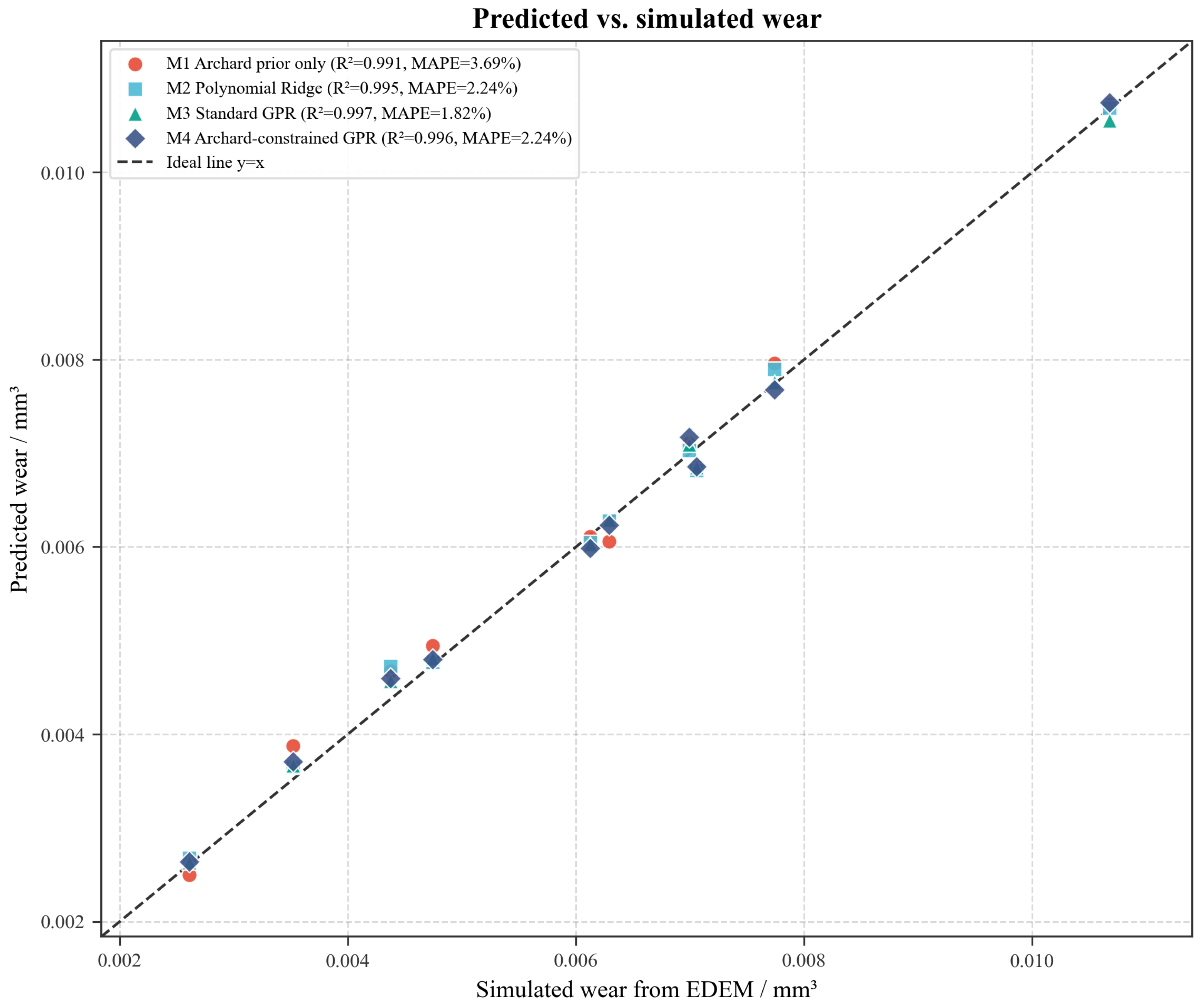
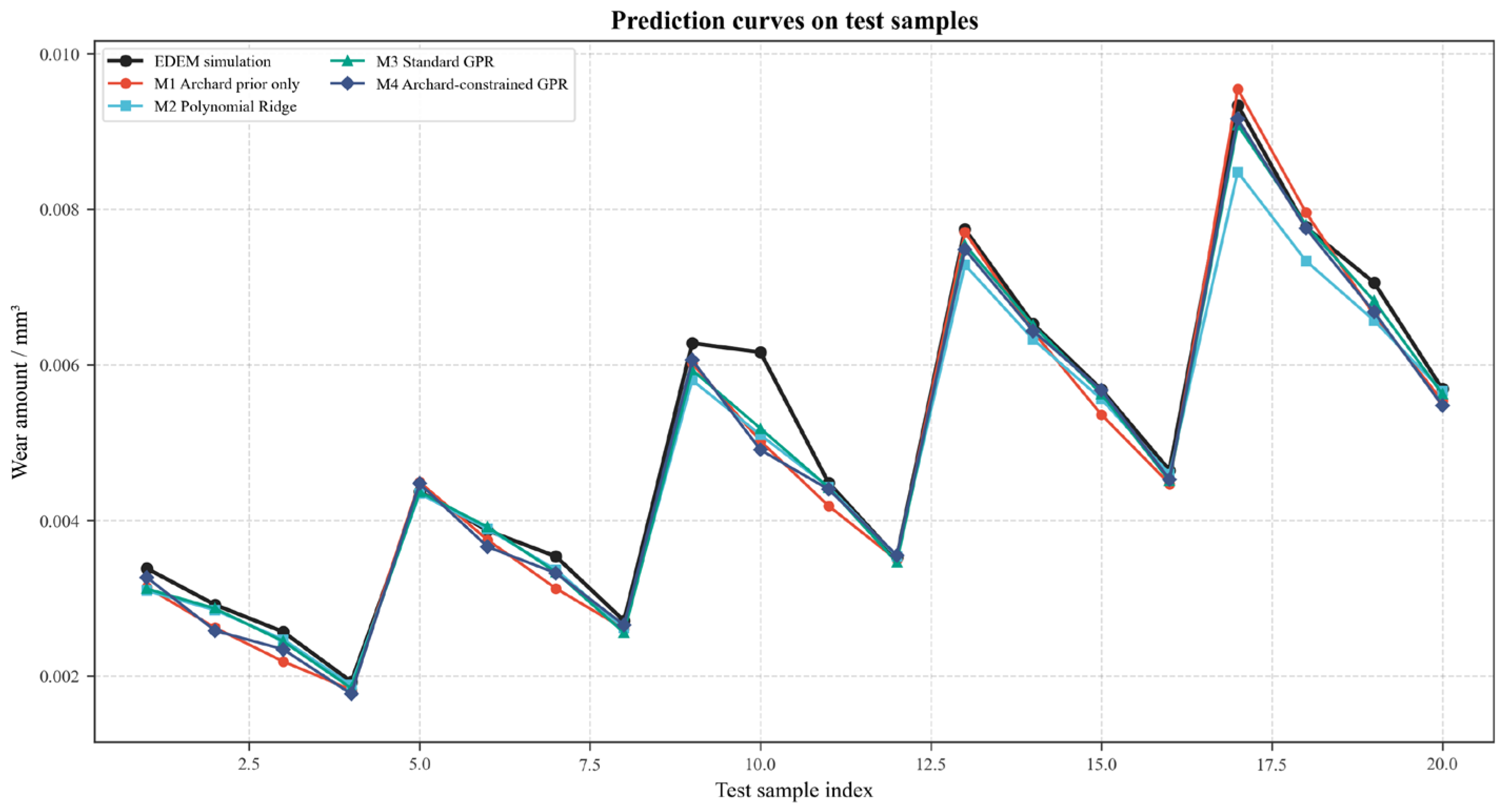
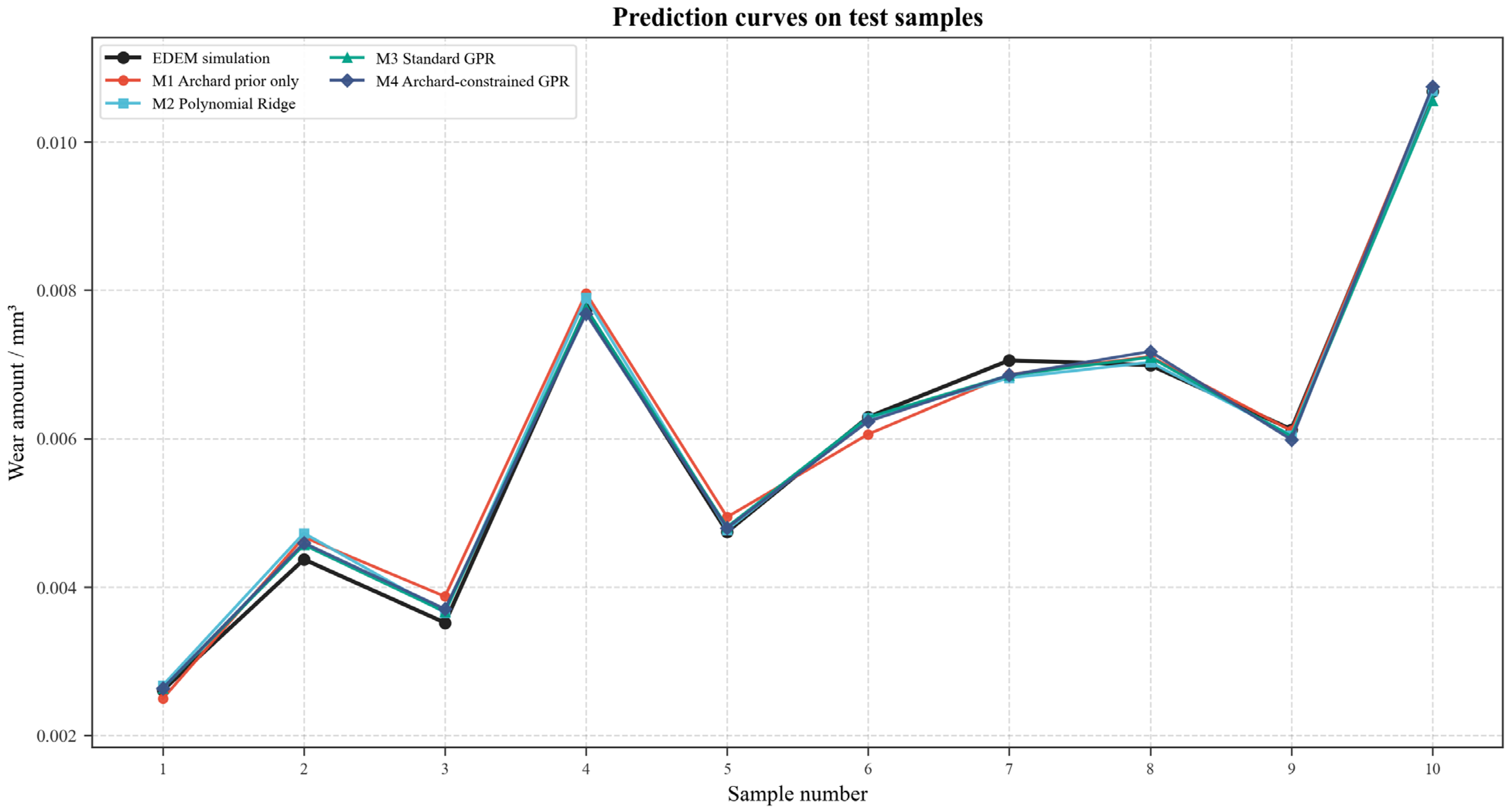
Figure 7 displays the scatter plots of predicted versus simulated wear values and shows that the predicted points of all models are generally distributed near the ideal 1:1 line, indicating no evident systematic prediction bias. Figure 8 further presents the prediction curves of test samples, which illustrate that M₂, M₃, and M₄ can accurately reproduce the wear variation trend obtained from EDEM simulation. Residual analysis indicates that the prediction errors of all models fluctuate slightly around zero, among which M₃ shows the smallest residual magnitude. The relative error curves also show that M₃ achieves lower prediction errors for most test samples within the interpolation domain.

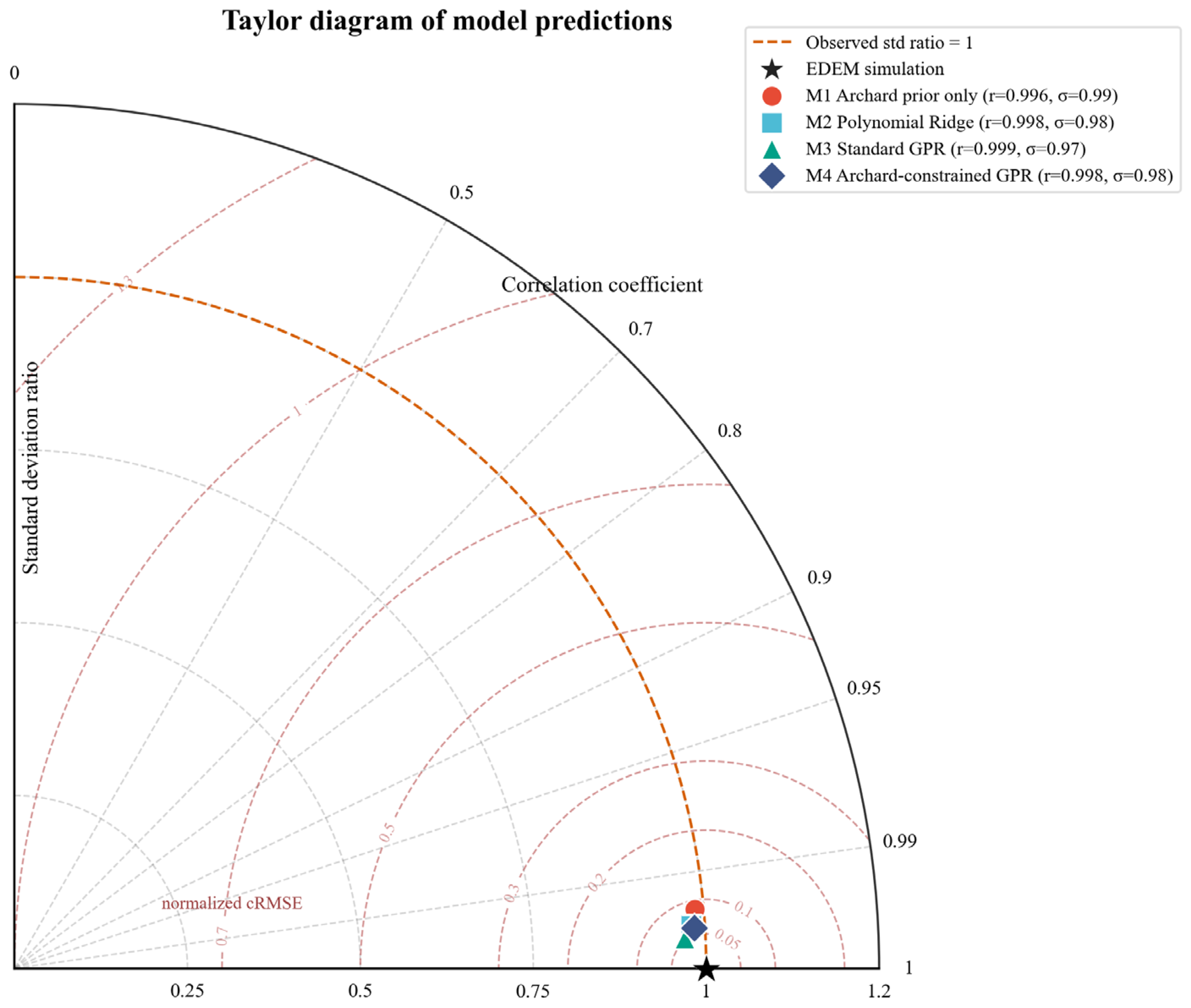
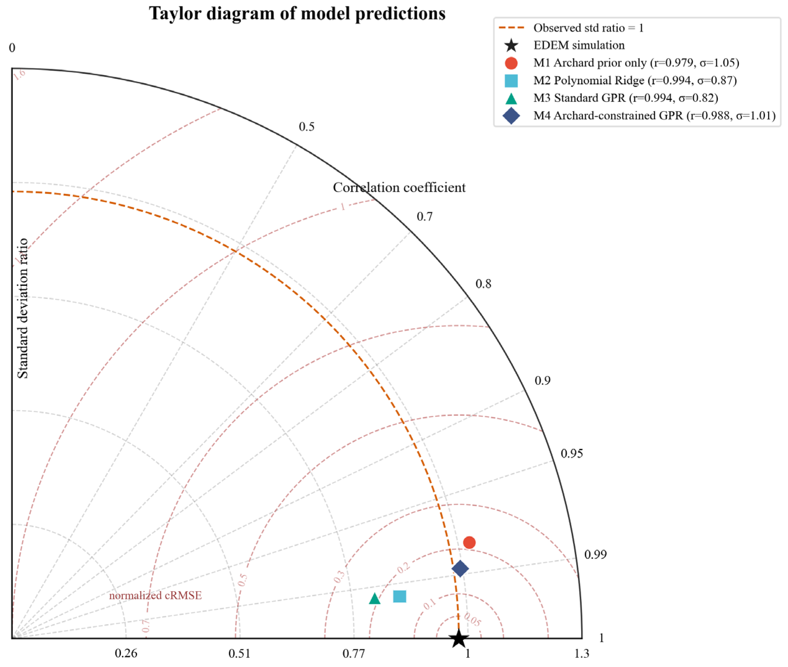
Figure 9 is the Taylor diagram of model performance, which simultaneously reflects the correlation coefficient, standard deviation matching degree, and centred RMSE. Under the representative random split interpolation condition, M₃ is closest to the EDEM simulation reference point in Figure 9, indicating that it has the highest linear correlation and its predicted standard deviation matches the distribution of simulated data most closely. M₄ is located close to M₃ in the diagram, suggesting that Archard-informed GPR also possesses competitive overall prediction performance under interpolation conditions.

It should be noted that the random split test is an interpolation-type validation, and the test samples do not exceed the parameter range of the training data; therefore, this result mainly demonstrates the local fitting ability of the models and cannot alone prove their extrapolation ability at unseen parameter levels.

3.3. Results of the Tillage-Depth Extrapolation Test

In the tillage-depth extrapolation test, which evaluates the extrapolation ability of the models under the boundary condition of greater tillage depth, samples with depths of 100, 125, 150, and 175 mm are used for training, and all 20 samples with a depth of 200 mm are used as the test set. The wear volume of the test set ranges from 0.005690 to 0.011278 mm³, with a mean value of 0.008092 mm³. The results are shown in

Table 6. Prediction performance under the tillage-depth extrapolation test.

Model	R2	RMSE/mm3	MAE/mm3	MAPE/%	Bias/mm3	PICP/%	MPIW/mm3
M1 Archard Prior Only	0.9528	0.000348	0.000284	3.43	0.000034	-	-
M2 Polynomial Ridge	0.5287	0.001099	0.001067	13.17	−0.001067	-	-
M3 Standard GPR	0.8524	0.000615	0.000515	5.90	−0.000515	100.0	0.002183
M4 Archard-Informed GPR	0.9752	0.000252	0.000214	2.68	0.000014	100.0	0.001598

.

Table 6 shows that M₄ achieves the highest prediction accuracy in tillage-depth extrapolation, with R², RMSE, MAE, MAPE, and Bias values of 0.9752, 2.52 × 10⁻⁴ mm³, 2.14 × 10⁻⁴ mm³, 2.68%, and 1.37 × 10⁻⁵ mm³, respectively. Compared with standard GPR, the RMSE of M₄ decreases from 6.15 × 10⁻⁴ to 2.52 × 10⁻⁴ mm³, a reduction of approximately 59.04%; its MAPE decreases from 5.90% to 2.68%; and its Bias decreases from −5.15 × 10⁻⁴ mm³ to nearly zero. Compared with cubic polynomial Ridge, the advantage of M₄ is more evident: M₂ has an R² of only 0.5287, MAPE of 13.17%, and Bias of −0.001067 mm³, indicating systematic underestimation.

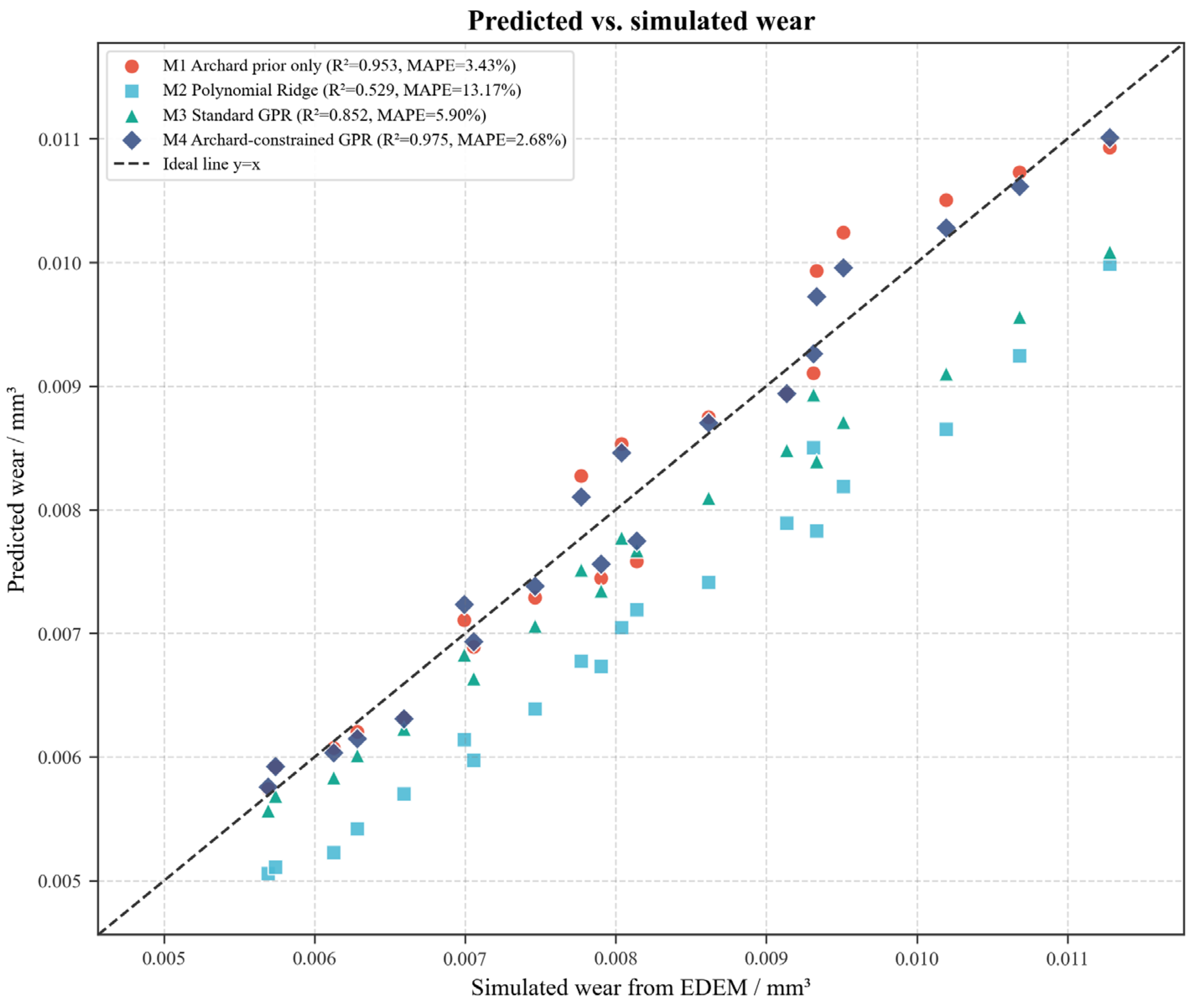
As shown in Figure 10, the predictions of M4 are generally closest to the 1:1 reference line, whereas M2 and M3 exhibit varying degrees of underestimation under the unseen 200 mm tillage-depth condition. The tillage-depth extrapolation results indicate that the Archard prior provides an effective constraint for load-dominated extrapolation. Increasing tillage depth enlarges the soil-cutting cross-section of the soil-engaging component; increases soil reaction force, normal contact load, contact frequency, and local compaction; and thereby affects the normal-load term and wear accumulation intensity in the Archard model. Existing DEM studies also show that tillage depth changes soil displacement, working resistance, and soil–component contact state [29,30,31,32]. In wear studies, normal load and sliding distance are key factors used by the Archard model to explain material loss [33,34]; therefore, under unseen high-depth conditions, M₄ can use the physical prior to provide a reasonable increasing wear trend, while the GPR residual term corrects local nonlinear errors, reducing the systematic bias of standard GPR and polynomial models during boundary extrapolation.

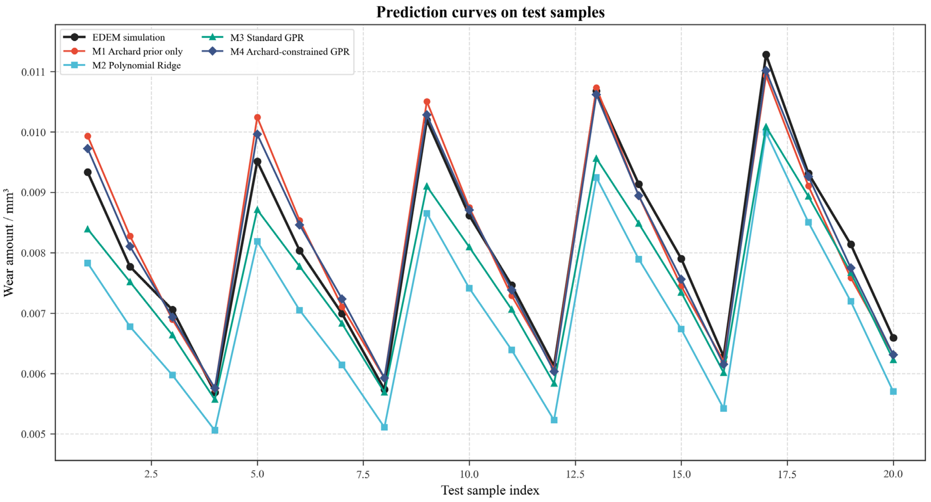
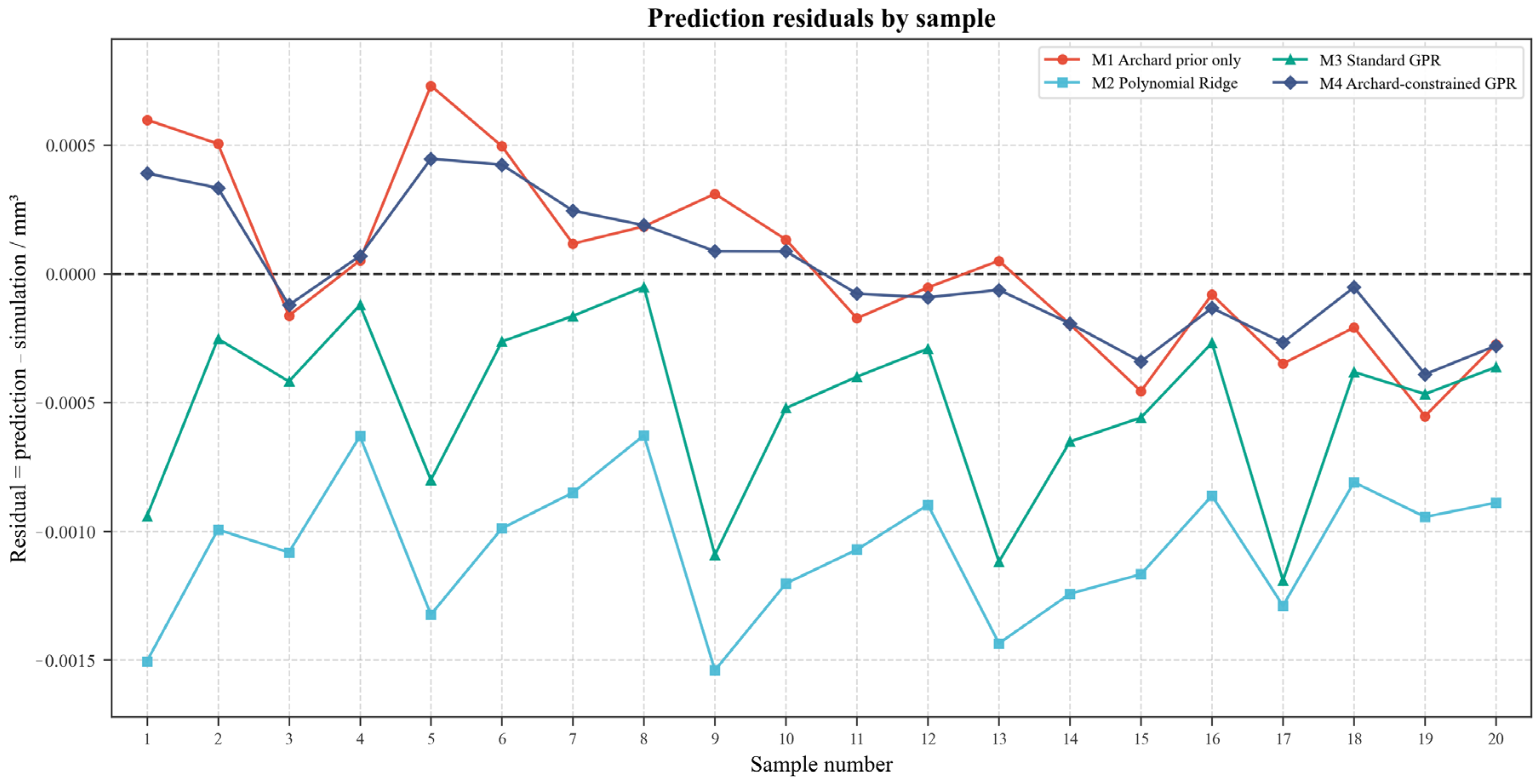
The sample-wise prediction curves in Figure 11 show that M2 systematically underestimates wear volume under the 200 mm tillage-depth condition, whereas the prediction curve of M4 follows the EDEM-simulated wear trend more closely. The corresponding residuals in Figure 12 further show that the residual curve of M2 is generally below the zero line and that M3 also exhibits predominantly negative residuals, indicating systematic underestimation by both models. In comparison, the residuals of M4 fluctuate only slightly around zero. Quantitatively, M3 has a Bias of −0.000515 mm³, whereas the Bias of M4 is only 0.000014 mm³. These results demonstrate that the Archard prior effectively corrects the systematic underestimation of standard GPR under high-depth extrapolation conditions.

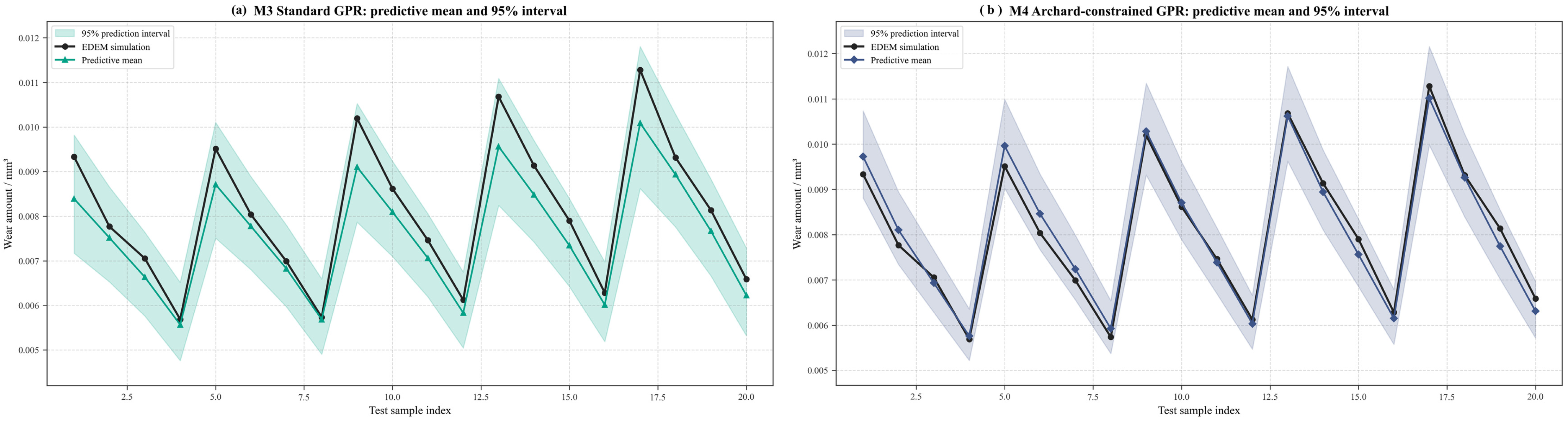
The 95% prediction intervals shown in Figure 13 indicate that both M3 and M4 cover all EDEM-simulated test values, corresponding to PICP values of 100%. However, the MPIW of M4 is 0.001598 mm³, which is lower than the value of 0.002183 mm³ obtained by M3. This result indicates that M4 provides a more compact prediction interval while maintaining complete empirical coverage. Thus, in the tillage-depth extrapolation scenario, the Archard prior improves not only the predictive-mean accuracy but also the uncertainty representation for unseen high-depth conditions.

The Taylor diagram in Figure 14 further supports the preceding results. Under the tillage-depth extrapolation condition, the model point of M₄ is closest to the EDEM simulation reference point, indicating that it outperforms the other models in correlation, standard deviation matching, and centred error. Combined with the prediction interval results, M₄ improves both predictive mean accuracy and interval compactness in this extrapolation scenario.

Overall, tillage depth directly affects the contact load, cutting resistance, and contact intensity between the soil-engaging component and soil, and is closely related to the normal-load term in the Archard model. Therefore, in the tillage-depth extrapolation scenario, the Archard prior provides GPR with a mean trend consistent with wear growth, enabling the model to maintain stable extrapolation under unseen high-depth conditions.

3.4. Results of the Tillage-Speed Extrapolation Test

In the tillage-speed extrapolation test, which evaluates the extrapolation ability of the models under the low-speed boundary condition, samples with speeds of 1.25, 1.50, 1.75, and 2.00 m/s are used as the training set, and all 20 samples with a speed of 1.00 m/s are used as the test set. The wear volume of the test set ranges from 0.001927 to 0.009334 mm³, with a mean value of 0.005008 mm³. The results are shown in

Table 7. Prediction performance under the tillage-speed extrapolation test.

Model	R2	RMSE/mm3	MAE/mm3	MAPE/%	Bias/mm3	PICP/%	MPIW/mm3
M1 Archard Prior Only	0.9695	0.000346	0.000255	5.68	−0.000203	-	-
M2 Polynomial Ridge	0.9627	0.000382	0.000253	4.36	−0.000249	-	-
M3 Standard GPR	0.9818	0.000267	0.000168	3.49	−0.000160	90.0	0.000598
M4 Archard-Informed GPR	0.9714	0.000335	0.000212	4.63	−0.000199	80.0	0.000617

.

Table 7 shows that M₃ performs best in tillage-speed extrapolation, with R², RMSE, MAE, and MAPE values of 0.9818, 2.67 × 10⁻⁴ mm³, 1.68 × 10⁻⁴ mm³, and 3.49%, respectively. M₄ has an R² of 0.9714, RMSE of 3.35 × 10⁻⁴ mm³, and MAPE of 4.63%; its overall accuracy is lower than that of M₃ but higher than that of M₁ in terms of MAPE. M₂ has an MAPE of 4.36%, lower than that of M₄, but its RMSE and Bias are worse than those of M₃, indicating that polynomial Ridge still has boundary prediction bias in this scenario.

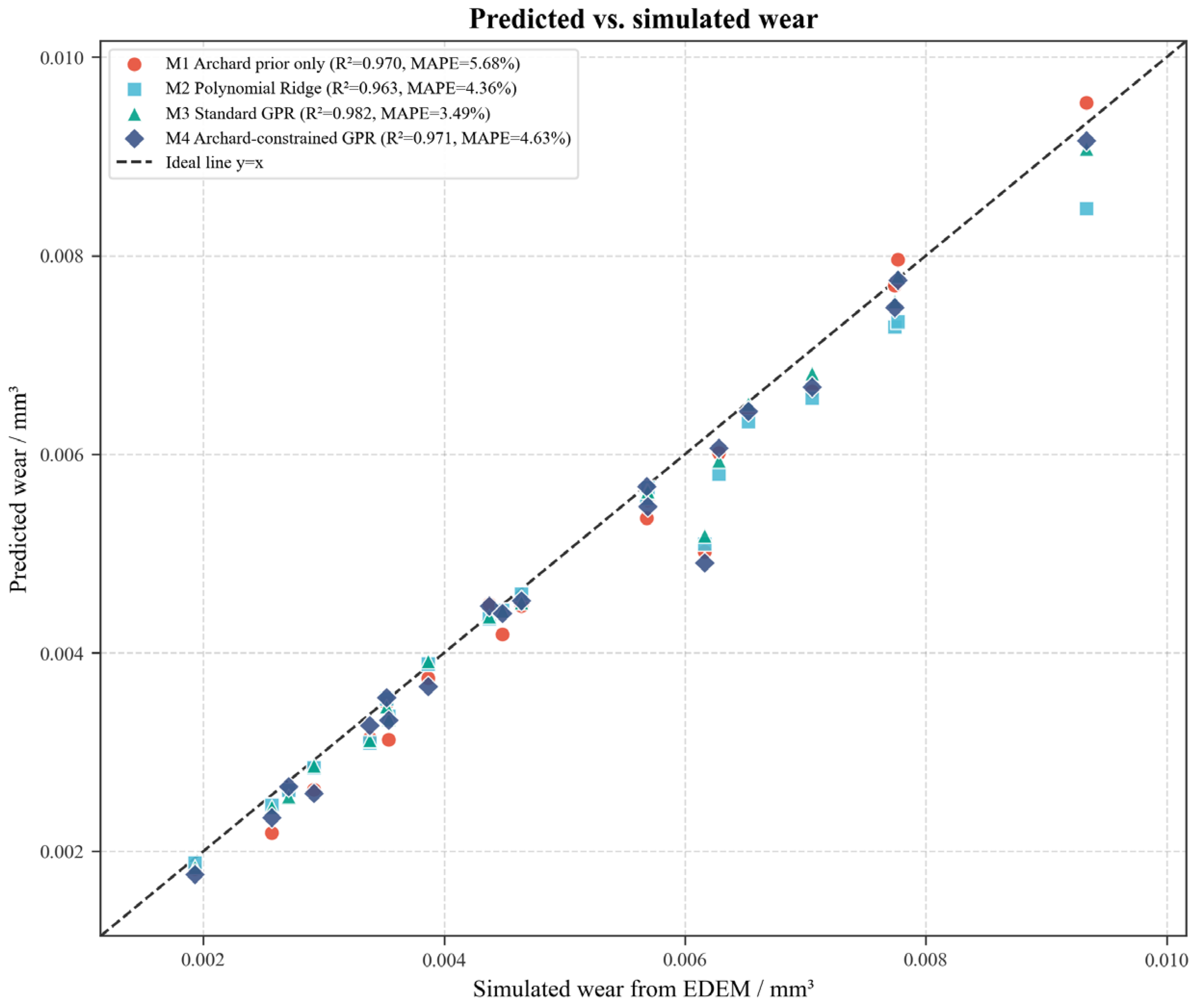
The predicted-versus-simulated comparison in Figure 15 shows that the predictions of all four models are predominantly located below the 1:1 reference line under the unseen 1.00 m/s tillage-speed condition, which is consistent with their negative Bias values. M3 has the Bias closest to zero, at −1.60 × 10⁻⁴ mm³, whereas M4 has a Bias of −1.99 × 10⁻⁴ mm³, suggesting that the Archard prior does not fully correct the systematic underestimation in low-speed extrapolation. A possible reason is that the effect of tillage speed on wear is not limited to changes in sliding distance per unit time; it also affects the particle-flow state, contact duration, contact frequency, particle-impact intensity, and soil-disturbance pattern. Previous DEM studies on tillage indicate that operating speed has complex effects on soil disturbance, resistance, and particle flow, and that soil–component contact responses may vary nonlinearly across different speed ranges [34]. Therefore, the Archard-inspired prior constructed from d, v, and α cannot fully represent the wear mechanism under low-speed boundary conditions.

The sample-wise prediction curves in Figure 16 show that all four models generally capture the variation in wear caused by tillage depth and penetration angle under the low-speed test condition. However, M1, M2, and M4 exhibit varying degrees of underestimation, whereas the prediction curve of M3 follows the EDEM-simulated wear curve more closely across the test samples. This difference indicates that the influence mechanism of tillage speed on wear volume does not fully conform to the simple power-law relationship assumed in the current Archard-inspired prior. In addition to affecting the relative sliding distance per unit time, tillage speed changes the soil-particle-flow state, contact duration, particle disturbance, contact frequency, and local impact behaviour. Consequently, a prior containing only a velocity-dependent term may be insufficient to describe wear variation at the low-speed boundary of 1.00 m/s.

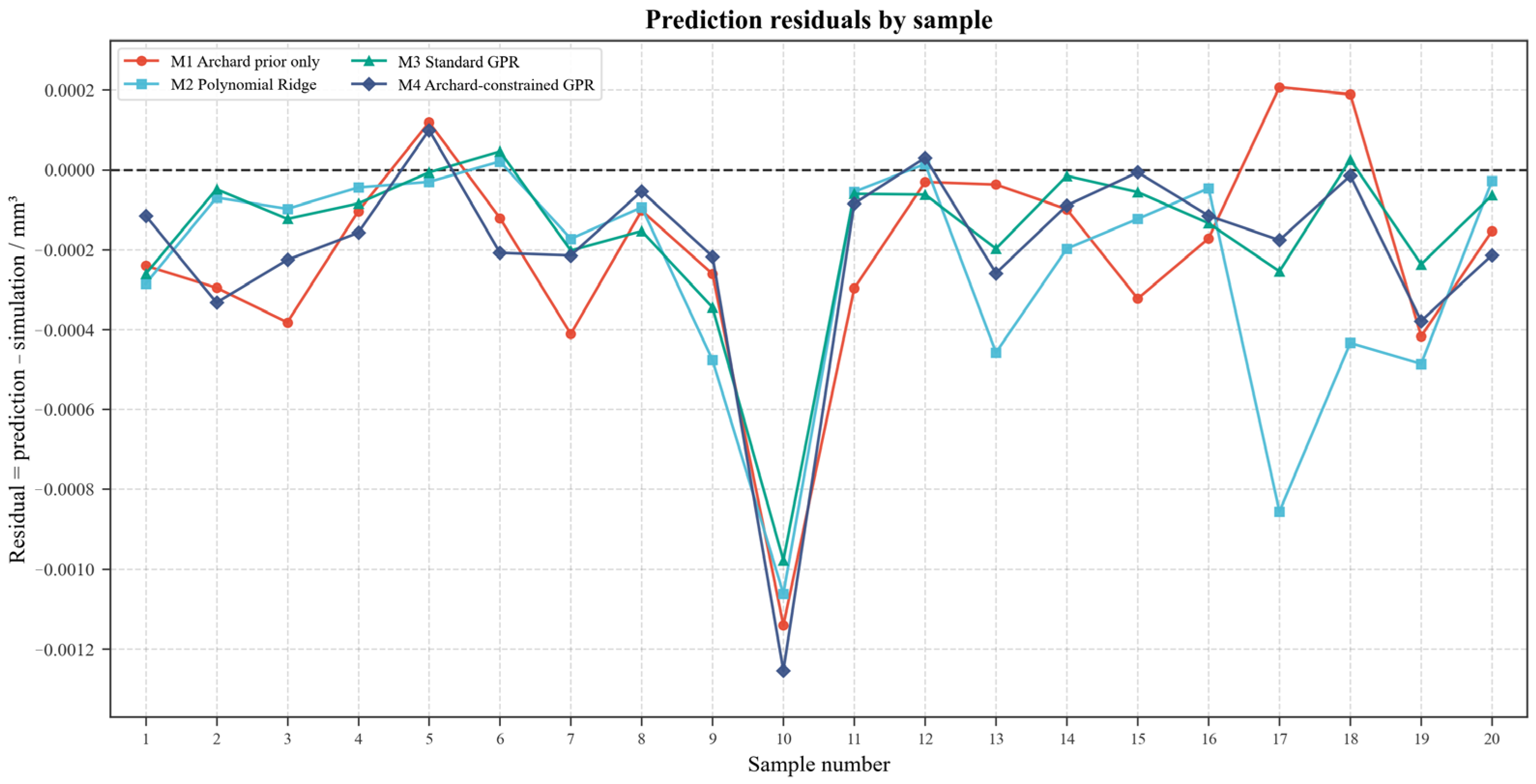
The prediction residuals in Figure 17 further show that M3 has the smallest overall residual magnitude and that its residuals are distributed more evenly around the zero line. By contrast, M1, M2, and M4 exhibit more persistent negative deviations, consistent with their systematic underestimation of wear volume. The relatively small and stable residuals of M3 indicate better data adaptability under the low-speed extrapolation condition. These results also suggest that the relationship between tillage speed and wear is less directly aligned with the Archard normal-load mechanism than the relationship between tillage depth and wear. Therefore, although the velocity term in the physical prior captures the general directional effect of speed, it does not adequately represent the nonlinear changes in soil flow and soil–component contact behaviour near the boundary of the investigated speed range.

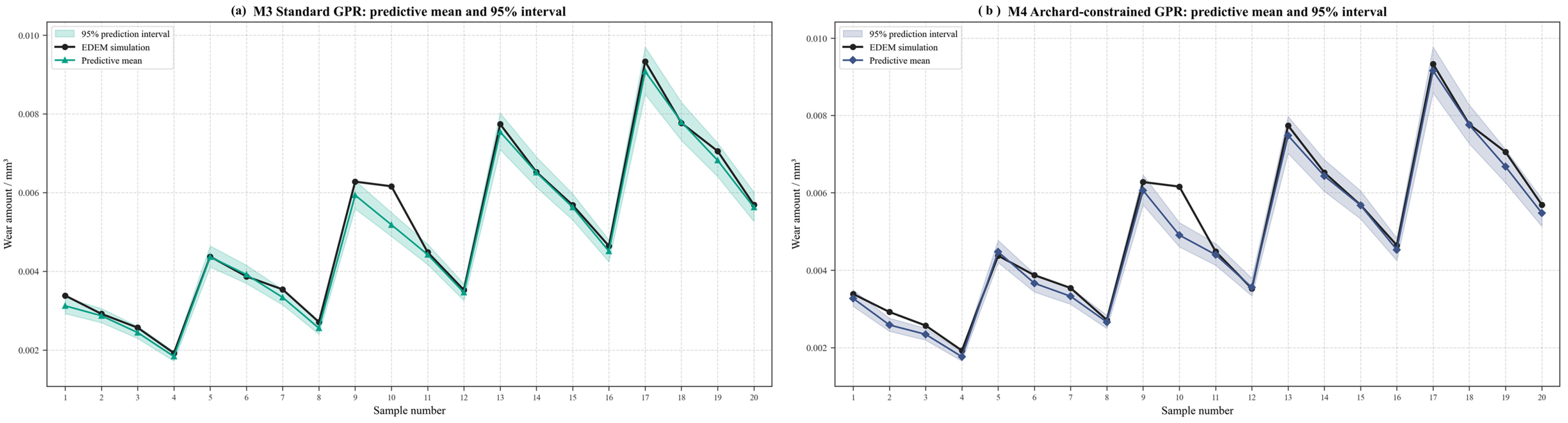
As shown in Figure 18, the 95% prediction intervals of M3 cover more of the EDEM-simulated test values than those of M4. Quantitatively, M3 has a PICP of 90% and an MPIW of 0.000598 mm³, whereas M4 has a PICP of 80% and an MPIW of 0.000617 mm³. Thus, M4 produces lower empirical coverage and a slightly wider prediction interval than M3, indicating that the physical prior does not improve the uncertainty representation of GPR in the tillage-speed extrapolation test. This result demonstrates that the benefit of the physical prior is conditional: when the extrapolated variable is strongly associated with the Archard normal-load term, the prior may improve prediction stability; however, when the variable affects wear mainly through indirect mechanisms such as particle-flow state and contact duration, a simple physical prior may be insufficient.

3.5. Results of the Penetration-Angle Extrapolation Test

In the penetration-angle extrapolation test, which evaluates the extrapolation ability of the models under the low-penetration-angle boundary condition, samples with angles of 30°, 45°, and 60° are used for training, and all 25 samples with an angle of 15° are used as the test set. The wear volume of the test set ranges from 0.003209 to 0.011278 mm³, with a mean value of 0.006620 mm³. The results are shown in

Table 8. Prediction performance under the penetration-angle extrapolation test.

Model	R2	RMSE/mm3	MAE/mm3	MAPE/%	Bias/mm3	PICP/%	MPIW/mm3
M1 Archard Prior Only	0.9283	0.000669	0.000606	9.96	0.000606	-	-
M2 Polynomial Ridge	−13.0385	0.009357	0.008646	129.15	0.008646	-	-
M3 Standard GPR	0.9293	0.000664	0.000540	7.24	−0.000486	96.0	0.001433
M4 Archard-Informed GPR	0.9283	0.000669	0.000606	9.96	0.000606	48.0	0.001276

.

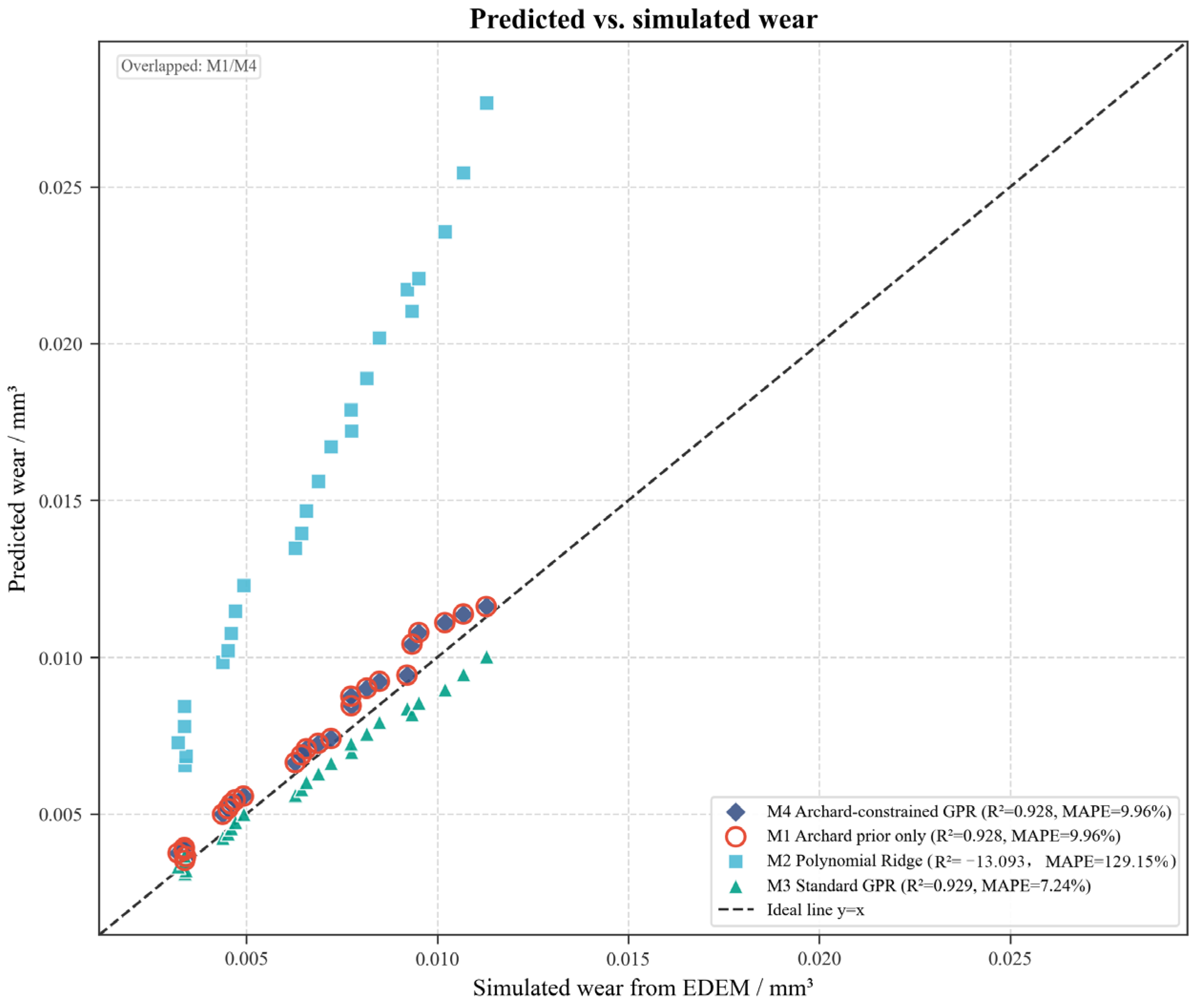
The predicted-versus-simulated comparison in Figure 19 shows that M3 provides the closest overall agreement with the EDEM-simulated values under the unseen 15° penetration-angle condition. The predictions of M1 and M4 exhibit similar positive deviations from the 1:1 reference line, whereas those of M2 deviate substantially above the reference line, indicating severe systematic overestimation. Quantitatively, M3 achieves R², RMSE, MAE, and MAPE values of 0.9293, 6.64 × 10⁻⁴ mm³, 5.40 × 10⁻⁴ mm³, and 7.24%, respectively. 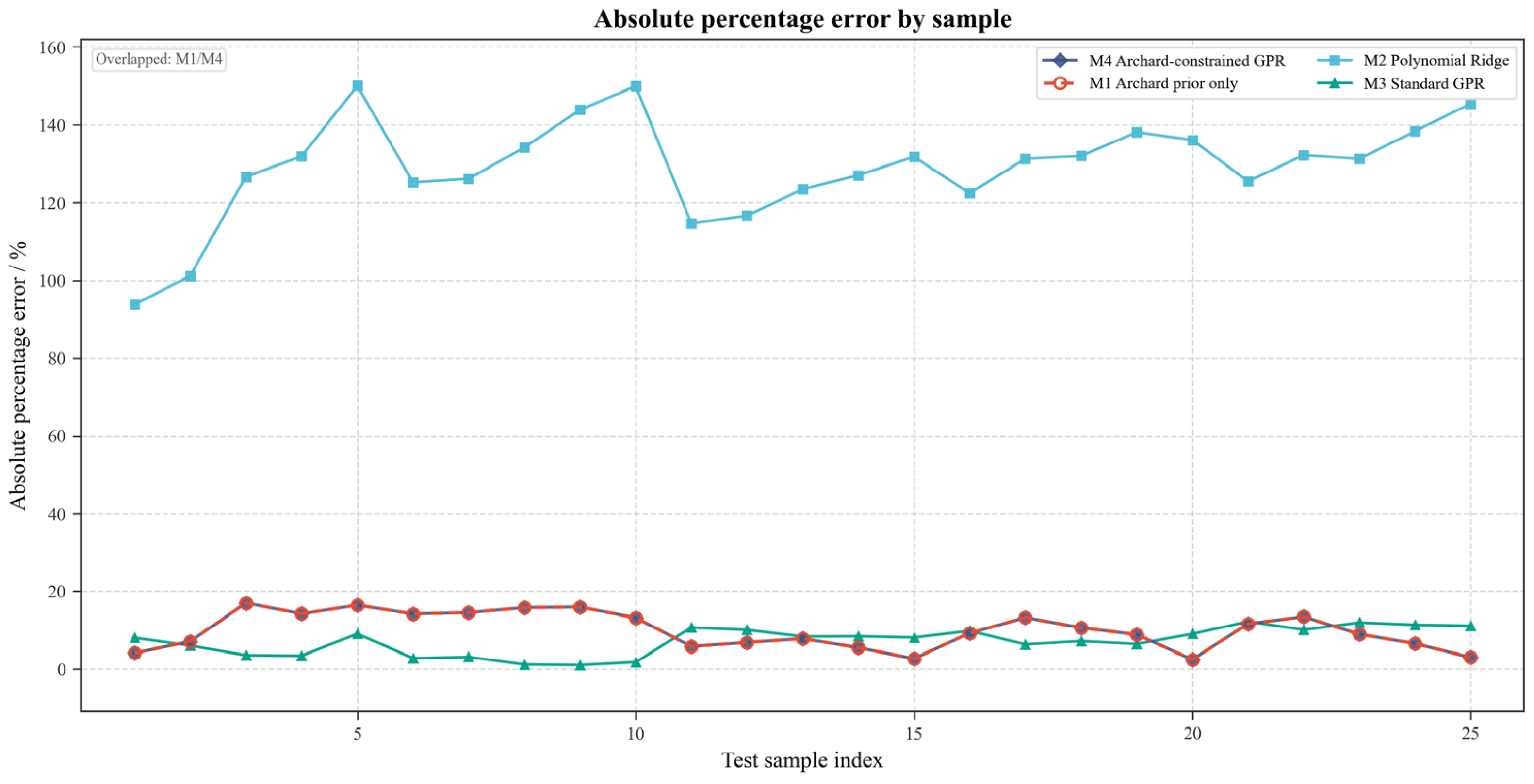By comparison, M4 has an R² of 0.9283, an RMSE of 6.69 × 10⁻⁴ mm³, and a MAPE of 9.96%, which are close to the results of M1. M2 performs particularly poorly, with an R² of −13.0385, a MAPE of 129.15%, and a Bias of 0.008646 mm³, confirming that the cubic polynomial response surface diverges when extrapolated to the unseen low-penetration-angle region.

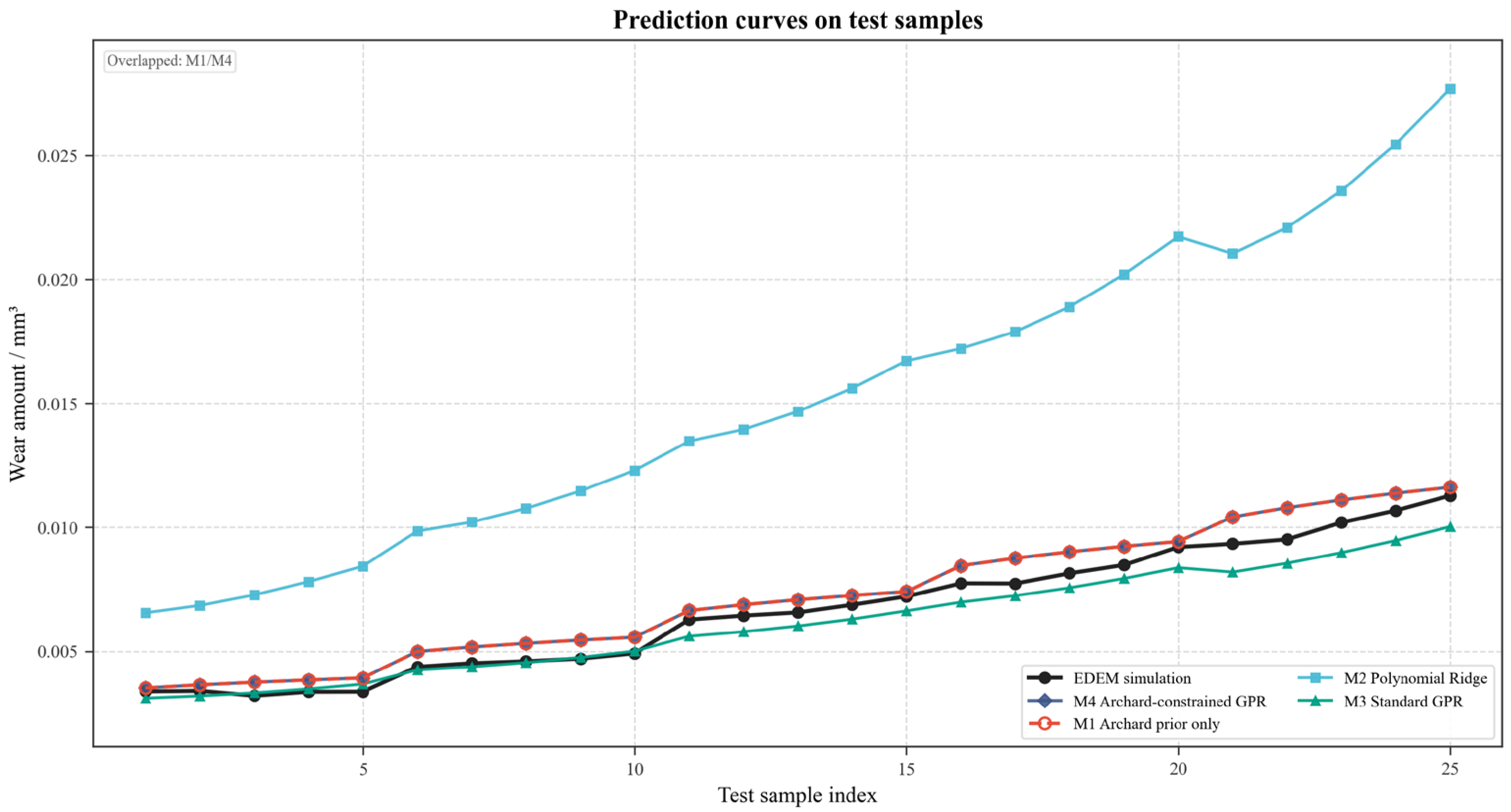
The sample-wise prediction curves in Figure 20 further demonstrate that M3 follows the EDEM-simulated wear trend more closely than the other models across the 25 test samples. In contrast, the prediction curve of M2 increases far above the simulated values, while the curves of M1 and M4 remain similar and generally overestimate wear. M4 does not outperform M3 in this extrapolation scenario mainly because the mechanism by which penetration angle influences wear is more complex than that of tillage depth. Penetration angle changes not only contact intensity but also penetration posture, soil-flow direction, effective contact area, local sliding path, and the location of abrasive action. DEM studies on narrow tines, furrow openers, and plough bodies show that component posture and penetration angle significantly affect soil-disturbance profiles, resistance fluctuations, and local contact processes [32,33]. Therefore, using exp(−β₃α) to describe the inhibitory effect of increasing penetration angle on wear can represent the general trend within the training range but cannot robustly extrapolate to the 15° low-penetration-angle boundary condition.

The relative-error comparison in Figure 21 provides further evidence of these performance differences. M2 exhibits extremely large relative errors across nearly all test samples, which is consistent with the divergence of its prediction curve. M3 generally produces the smallest and most stable relative errors, whereas M1 and M4 show similar but larger error levels. These results indicate that the GPR residual correction in M4 cannot fully compensate for the structural bias introduced by the penetration-angle term of the physical prior. Although the current Archard-inspired prior correctly represents the overall direction of the penetration-angle effect, it is not sufficiently flexible to describe the nonlinear changes in contact posture, soil flow, local sliding, and abrasive-action location near the low-angle boundary. Consequently, the prediction accuracy of M4 depends strongly on whether the assumed physical-prior form remains valid outside the training range.

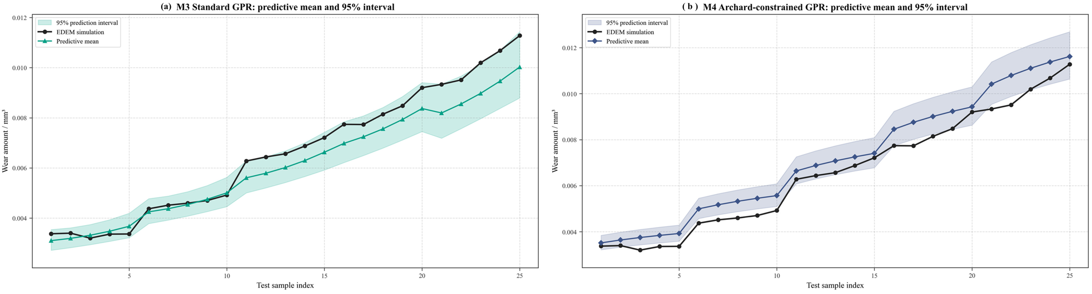
The 95% prediction intervals shown in Figure 22 further support this interpretation. M3 achieves a PICP of 96% with an MPIW of 0.001433 mm³, indicating that its intervals provide approximately nominal coverage of the EDEM-simulated test values. By contrast, M4 has a narrower MPIW of 0.001276 mm³ but a PICP of only 48%, and many simulated values fall outside its prediction intervals. The narrower interval of M4 is therefore not an advantage but evidence of severe undercoverage and overconfidence. This behaviour is consistent with structural bias in the penetration-angle term and incomplete propagation of uncertainty in the Archard-prior parameters. A possible reason is that the current model mainly propagates the uncertainty of the GPR residual, whereas the uncertainty associated with the fitted physical-prior parameters is not fully considered. For variables strongly affected by contact posture, such as penetration angle, future studies should incorporate EDEM-derived microphysical features, including normal contact force, tangential sliding distance, frictional work, contact area, and contact frequency, to improve the adaptability of the physical prior to boundary conditions. Overall, the results show that M2 is unsuitable for penetration-angle boundary extrapolation, M3 is relatively stable, and the performance of M4 depends on the accuracy of the assumed physical-prior form.

The boundary tests should not be read as evidence that one model is universally superior; M₄ was most accurate only for the 200 mm tillage-depth test, whereas M₃ was more accurate for the 1.00 m/s speed test and the 15° penetration-angle test. This pattern is consistent with a prior that is more directly aligned with load-related depth changes than with the coupled flow and contact-posture changes induced by speed and angle.

3.6. Overall Comparison of Model Performance

The model ranking was scenario-dependent: M₃ provided the best interpolation performance in the representative random split and was more stable in speed and penetration-angle extrapolation; M₄ provided the best result in the depth extrapolation case, where the withheld variable was most closely related to load and contact intensity; M₂ was competitive for interpolation but unstable outside the training domain; and M₁ preserved a simple monotonic trend but lacked residual correction. The results therefore support a conditional use of the prior-guided model rather than a claim of general superiority.

4. Discussion

4.1. Predictability and Validation Scope of the EDEM Dataset

The 100-sample full-factorial dataset is small relative to datasets used for deep learning, but it is dense for a three-dimensional regular design, explaining why GPR and regularized polynomial regression achieved high interpolation accuracy. Repeated random splits showing consistently high interpolation performance across 30 independent trials, with all data-driven models achieving mean R² above 0.99 and mean MAPE below 3%, demonstrate that this conclusion is not driven by one favourable set of ten test samples.

The prediction target is the total wear volume generated by one EDEM configuration, rather than a direct measurement of ploughshare mass loss or service life. Particle properties, contact model parameters, cohesion, boundary conditions, mesh representation, and the fixed wear coefficient affect the target values. The surrogate is therefore valid as an emulator of the calibrated simulation configuration; transfer to field use requires independent soil-bin or field calibration, particularly for the absolute wear-volume scale.

4.2. Conditional Benefit in Tillage-Depth Extrapolation

M₄ reduced the depth extrapolation RMSE relative to standard GPR and preserved the increasing wear trend at 200 mm. Tillage depth increases the engaged soil cross-section and is expected to increase soil reaction force and normal contact intensity; therefore, depth is the most direct proxy among the three selected operating variables for the load term that motivates the Archard-inspired prior. Mechanistically, a larger depth increases the disturbed soil volume and can increase both the number and persistence of particle–surface contacts. Over the fixed 10 m travel distance, these effects are expected to raise the cumulative normal-load–sliding contribution accumulated by the EDEM wear model, which is consistent with the observed increase in total wear volume.

A stationary GPR fitted only to depths of 100–175 mm may revert toward its training-domain mean near the upper boundary. The monotonic prior supplies a directional trend, while the residual GPR corrects local nonlinear departures, explaining why a prior that does not improve interpolation can still improve a specific extrapolation direction. The result should nevertheless be described as evidence from one withheld depth level, not as general proof of load extrapolation.

4.3. Prior Bias in Speed and Penetration-Angle Extrapolation

The same prior did not improve speed or penetration-angle extrapolation. Speed changes not only sliding distance per unit time but also particle kinetic energy, contact duration, contact frequency, impact intensity, and the soil flow pattern. Penetration angle changes tool posture, effective contact area, pressure distribution, local sliding path, and the location of abrasive action. These coupled mechanisms are not represented by a single power-law speed term or exponential angle term. Because the simulated travel distance was fixed at 10 m, speed does not simply scale the nominal travel distance; instead, it modifies time-dependent contact dynamics, including impact severity, particle rearrangement, and force fluctuations. For penetration angle, the redistribution of contact pressure and sliding paths across the working surface means that total wear integrates competing local increases and decreases, which can violate the assumed simple monotonic trend.

The 48% PICP of M₄ in the 15° test is particularly important, as it shows that a biassed prior can shift the predictive mean while the residual GPR still reports a narrow variance, producing overconfident intervals. A physically motivated prior is therefore not automatically a safer prior: its structural adequacy must be checked for each extrapolated variable.

4.4. Circularity and Interpretation of the Archard-Inspired Prior

The EDEM wear outputs were generated using an Archard-type wear model, and the surrogate also contains an Archard-inspired trend. This structural consistency may contribute to the observed depth extrapolation gain. The result demonstrates efficient emulation of an Archard-based DEM response, but it does not by itself demonstrate improved physical understanding or transfer to wear data generated by another wear law.

The present study therefore treats the prior as a transparent inductive bias rather than as independent physical validation. Stronger generalization evidence would require comparison with an alternative wear formulation, variation in the wear coefficient or DEM calibration, or independent experimental wear data; until such evidence is available, claims are restricted to the current simulation framework.

4.5. Ablation and Baseline Scope

The prior-only, data-only GPR, and prior-plus-residual models form a direct ablation of the proposed architecture: M₁ demonstrates that the prior alone is too simple for accurate prediction; M₃ shows the flexibility of the residual learner without the operational prior; and M₄ reveals the combined effect. The comparison shows that residual correction is essential and that prior structure is useful only in the depth boundary case.

Cubic polynomial Ridge was retained as a conventional response-surface baseline and was competitive for interpolation but diverged in the penetration-angle extrapolation. Broader comparisons with SVR or tree ensembles would be useful for a benchmark study, but they are not necessary to isolate the effect of the prior–residual architecture.

4.6. Uncertainty Calibration

GPR prediction intervals should be evaluated by both coverage and sharpness, as high coverage with very wide intervals is not informative, whereas a narrow interval with low coverage is overconfident. The reliability diagram and multi-level PICP/MPIW results, which reveal markedly divergent calibration behaviours across the three extrapolation scenarios, provide a more complete assessment than a single nominal 95% interval. Here, calibration refers to the empirical agreement between a nominal interval level and the fraction of held-out EDEM responses covered across a test set; it is not a per-sample guarantee. The reported intervals quantify conditional surrogate uncertainty under the fixed DEM configuration and do not include uncertainty in DEM parameters, the wear coefficient, fitted prior parameters, or experimental variability.

The current M₄ formulation propagates the residual GPR variance but treats the fitted prior parameters as fixed. Bootstrap or Bayesian estimation of the prior parameters, model averaging, and explicit representation of DEM response uncertainty are possible extensions; these additions are especially important when the prior form is uncertain at a boundary.

4.7. Practical Implications

Within the calibrated EDEM configuration, the surrogate can replace many repeated simulations for rapid comparison of relative wear among operating combinations. The prior-guided model is most defensible when screening high-depth, load-dominated conditions close to the investigated boundary. For speed and penetration-angle screening, standard GPR should be retained as a competing model, and disagreement between M₃ and M₄ can be used as a warning that additional EDEM simulations are needed.

4.8. Limitations and Future Work

The main limitations are the single DEM configuration, fixed wear coefficient, absence of independent experimental wear measurements, and use of total wear volume rather than local wear evolution. Moreover, the operational prior does not directly use accumulated normal force, sliding distance, frictional work, contact area, or contact frequency, and the full-factorial design is transparent but may be less efficient than space-filling or adaptive sampling for higher-dimensional problems.

Future work should calibrate the DEM and wear coefficient against soil-bin or field measurements, propagate parameter and simulation uncertainty, include local wear maps or microphysical contact descriptors, and test the framework under alternative soil states, tool geometries, and wear formulations. These steps are required before general claims about service-life prediction or cross-domain transfer can be made.

5. Conclusions

This study developed a residual-learning surrogate for the total wear volume generated by an EDEM ploughshare model. The prior is an Archard-inspired operational-parameter trend rather than a direct use of normal load and sliding distance; therefore, the M₁–M₃–M₄ comparison evaluates the effect of a simplified prior, a data-only GPR, and their combination.

Within the sampled domain, standard GPR and polynomial Ridge were at least as accurate as the prior-guided model: across 30 independently repeated 90%/10% random training–test splits, the former exhibited a modest yet statistically significant advantage in RMSE over the Archard-informed GPR as verified by a paired Wilcoxon signed-rank test (p = 0.018), while both data-driven models maintained consistently high interpolation performance with mean R² values above 0.99. Thus, the Archard-inspired prior did not provide a general interpolation advantage.

The prior-guided model performed best in the 200 mm tillage-depth extrapolation test, with R² = 0.9752, RMSE = 0.000252 mm³, and MAPE = 2.68%, supporting a conditional benefit for the load-dominated depth direction. Standard GPR remained more accurate in the speed and penetration-angle tests, while the 48% coverage of M₄ in the penetration-angle test showed that prior bias can also produce overconfident uncertainty estimates.

Accordingly, the proposed model should be used as a scenario-dependent EDEM surrogate, not as a universally superior or experimentally validated wear predictor. Its engineering application depends on DEM calibration, the selected wear coefficient, uncertainty calibration, and future validation using microphysical DEM outputs and soil-bin or field wear measurements.