Deep Learning for Hourly FAO-56 PM-Derived Crop Evapotranspiration Estimation Using a Transformer Encoder Approach for Data-Driven Irrigation Management in Tropical Horticulture

Abstract

Accurate hourly crop evapotranspiration (ETc) estimation is important for data-driven irrigation management support in tropical horticulture, yet existing approaches are constrained by data requirements and an inability to capture multi-scale temporal dynamics. This study proposes a Transformer encoder model for one-step-ahead hourly FAO-56 PM-derived ETc estimation in a durian orchard in Chanthaburi Province, Eastern Thailand, using 36,528 hourly meteorological observations obtained from the Visual Crossing Weather API for the orchard location over four years, with ETc computed from these inputs using the FAO-56 Penman–Monteith equation. The model employs a 168-h (7-day) look-back window, three stacked encoder blocks with multi-head self-attention ($h=8$, $d_{\mathrm{model}}=128$), and five meteorological input features (air temperature, relative humidity, solar radiation, wind speed, and ETc). A SARIMA$(2,1,2){(1,0,0)}_{24}$ model trained on the same dataset served as the statistical baseline. The Transformer achieved an RMSE of 0.0308 mm/h, MAE of 0.0188 mm/h, and $R^2$ of 0.9018 on the 168-h test set, outperforming SARIMA (RMSE = 0.0717, MAE = 0.0593, $R^2$ = 0.4688), representing a 57.0% reduction in RMSE, a 68.3% reduction in MAE, and a 92.4% improvement in $R^2$. The Transformer also achieved a daytime-only RMSE of 0.0414 mm/h vs. 0.0791 mm/h for SARIMA, and a daily cumulative ETc MAE of 0.1599 mm/day vs. 0.5901 mm/day, demonstrating superior accuracy during agronomically critical periods. The Transformer accurately reproduced both the 24-h diurnal cycle and the 7-day weekly pattern of ETc, whereas SARIMA exhibited a damped amplitude response. A recursive 168-h heuristic simulation demonstrated that the model generates physically plausible ETc patterns under an approximated meteorological scenario, suggesting the approach warrants further investigation as a component of future irrigation decision-support research. These results highlight the potential of Transformer-based deep learning for site-specific, proof-of-concept ETc estimation from meteorological inputs in tropical fruit production, pending validation across diverse sites and seasons.

1. Introduction

Accurate estimation of crop evapotranspiration (ETc) is fundamental to precision irrigation management, enabling farmers to match water supply with actual crop demand and thereby improve water-use efficiency, reduce energy costs, and sustain agricultural productivity under increasing water scarcity [1]. In tropical fruit cultivation, where irrigation scheduling is particularly sensitive to diurnal and seasonal fluctuations in atmospheric demand, reliable hourly ETc estimates are important for supporting data-driven irrigation management in drip and micro-irrigation systems [2]. Durian, Thailand’s most economically significant tropical fruit, is cultivated extensively in the Eastern region, where prolonged dry spells and erratic rainfall patterns make data-driven irrigation decisions increasingly critical for maintaining yield and fruit quality [3].

The Food and Agriculture Organization (FAO) Penman–Monteith (PM) equation remains the internationally recommended standard for computing reference evapotranspiration (ETo) [4]. Although physically well-founded, its operational application is impeded by the requirement for complete sets of meteorological inputs, net radiation, air temperature, humidity, and wind speed, which are frequently unavailable and subject to measurement gaps at the farm level, particularly in developing regions [5]. Moreover, ETc estimates rely on empirically derived crop coefficients ($K_c$) that must be locally calibrated and periodically updated, introducing additional uncertainty in dynamic tropical environments [6]. These limitations have motivated a growing body of research into data-driven approaches capable of learning ETc dynamics directly from meteorological observations, without explicit physical parameterization.

Machine learning (ML) and deep learning (DL) methods have been widely explored as alternatives or complements to physics-based ETc models. Shallow ML approaches including support vector regression, random forests, and extreme gradient boosting have demonstrated competitive accuracy relative to PM estimates when trained on locally collected meteorological data [7,8]. Among sequential models, Long Short-Term Memory (LSTM) networks and Gated Recurrent Units (GRU) have been particularly effective for short-term forecasting, owing to their ability to capture nonlinear temporal dependencies across multi-day look-back windows [9,10,11,12]. However, recurrent architectures process sequences step-by-step and may struggle to directly exploit long-range periodic patterns—such as the pronounced 24-h diurnal and 7-day weekly cycles that characterize weather in tropical orchards—because information from distant timesteps must propagate through many sequential hidden states [12,13].

Statistical time-series models, notably the Seasonal Autoregressive Integrated Moving Average (SARIMA), have also been applied to short-term ETc and reference ET forecasting [14,15]. SARIMA is interpretable and computationally efficient, but it is inherently univariate, relying solely on the historical ETc record and unable to assimilate concurrent meteorological drivers such as solar radiation and humidity as auxiliary features. Furthermore, SARIMA assumes linear dynamics and a fixed seasonal structure, which can inadequately represent the complex non-stationary behavior of ETc under variable cloud cover and intermittent rainfall in tropical climates [9,14,15].

The Transformer architecture, originally introduced by Vaswani et al. for natural language processing [16], has recently demonstrated strong performance on multivariate time-series forecasting tasks in agricultural and environmental domains. Its multi-head self-attention mechanism allows the model to simultaneously relate any pair of timesteps within the input window, regardless of their temporal distance, making it well-suited to capturing both short-term diurnal transitions and longer weekly periodicities without the information-decay constraint of recurrent networks [17,18]. Compared with LSTM-based models, Transformer encoders are also more amenable to parallelization, facilitating training on large meteorological datasets collected over multi-year periods [19,20].

Despite these promising properties, the application of Transformer models to hourly ETc estimation in tropical horticultural settings remains largely unexplored, and a direct comparison with SARIMA as a statistical baseline under identical data conditions has not been reported. Most existing studies focus on daily and sub-daily reference ET in temperate climates, using meteorological station data rather than location-specific weather API data [21,22]. The present study addresses this gap through a site-specific proof-of-concept evaluation; given the single-site design, PM-derived target variable, single chronological holdout period, and heuristic simulation component, it is not intended as a validated operational system, and its findings should be interpreted accordingly.

To address these gaps, this study proposes a Transformer encoder model for hourly ETc estimation in a durian orchard in Chanthaburi Province, Eastern Thailand, using 36,528 hourly meteorological observations obtained from the Visual Crossing Weather API for the orchard location over four years, with ETc computed using the FAO-56 Penman–Monteith equation. The model employs a look-back window of 168 h (7 days) and stacked multi-head self-attention blocks to capture both diurnal and weekly ETc dynamics. A SARIMA$(2,1,2){(1,0,0)}_{24}$ model trained on the same data serves as the statistical baseline.

To the best of the authors’ knowledge, no previous study has applied a Transformer encoder model to hourly crop ETc estimation in a tropical orchard setting using meteorological data from a weather API. Most existing studies address daily and sub-daily reference ET in temperate climates with standard weather station data [6,9], leaving a gap in exploratory evaluations of deep learning approaches for hourly ETc estimation in tropical fruit production systems. The principal contributions of this work are as follows:

• A multivariate Transformer encoder architecture is developed and evaluated for one-step-ahead hourly FAO-56 PM-derived ETc estimation at a single tropical orchard location, using meteorological data obtained from a weather API. The results suggest that a 168-h self-attention window can reproduce the 24-h diurnal cycle and 7-day weekly pattern of ETc at this site and test period; however, these findings are specific to the single site and episode evaluated and cannot be generalised without further validation.
• An exploratory and structurally unbalanced comparison between the proposed multivariate Transformer and a univariate SARIMA baseline is conducted under identical train-test partitioning. Because the Transformer receives five meteorological input features while SARIMA operates on the ETc series alone, the observed performance difference reflects a combination of architectural, input, and context-length factors and cannot be attributed to the self-attention mechanism alone. This comparison is therefore reported as an initial exploratory evaluation rather than a controlled architectural assessment.
• A recursive 168-h heuristic simulation is implemented as a visually assessed feasibility demonstration under approximated meteorological inputs, in which future meteorological variables are approximated using observed values from 72 h prior. This exercise is not a validated forecasting procedure; it illustrates only that the model can maintain physically plausible ETc patterns under a simplified meteorological approximation. Its utility for irrigation planning remains to be established through field-based investigation involving independently measured ETc and real forecast weather inputs.

2. Materials and Methods

2.1. Study Area and Data Collection

The dataset used in this study comprises hourly meteorological data obtained from the Visual Crossing Weather API https://www.visualcrossing.com/weather-api (accessed on 23 October 2025) for the location of a durian orchard in Chanthaburi Province, Eastern Thailand (approximately 12°36′ N, 102°6′ E). Data were retrieved continuously from August 2021 to September 2025, yielding a total of 36,528 hourly observations. The retrieved variables included air temperature (°C), relative humidity (%), solar radiation (W/${\mathrm{m}}^2$), and wind speed (m/s). Hourly crop evapotranspiration (ETc, mm/h), which served as the target variable, was computed externally from these four meteorological inputs using the FAO–56 Penman–Monteith equation. The processed dataset and a visualization dashboard are publicly available at https://weather-31ba2.web.app/home (accessed on 23 October 2025). Note that this link directs to a web platform hosted on a separate server that retrieves and displays data for the above coordinates; the geographic reference of the data query is fixed to the study orchard location stated above.

2.2. Data Preprocessing

Raw sensor readings were parsed by combining the date and hour fields into a unified datetime index and sorted in chronological order. The hourly time series obtained from the Visual Crossing Weather API was largely complete over the four-year study period. Anomalous values were identified through visual inspection of the parsed hourly time series, including implausible readings that fell outside the physically expected range for each meteorological variable. Such values accounted for less than 0.5% of the total 36,528 observations and were retained without modification or imputation. Given the negligible proportion relative to the full four-year record, their influence on sliding-window construction and model training is considered minimal. Five input features were selected for model training, namely air temperature, relative humidity, solar radiation, wind speed, and ETc. All features were normalized to the interval $[0,1]$ using Min–Max scaling [23]. The scaling function is presented in Equation (1), where x is the original value and $x^{\prime }$ is the scaled value.

$$x^{\prime }={\displaystyle \frac{x-x_{min}}{x_{max}-x_{min}}}$$

(1)

This standard normalization formula maps each feature value to the interval $[0,1]$ and is widely used in deep learning preprocessing [23].

To prevent data leakage, the dataset was first partitioned chronologically into a training subset (all observations except the final 168 h) and a test set (the last 168 h, corresponding to 7 days) before any scaling was applied.The Min–Max scaler was then fitted exclusively on the training subset and applied without modification to the test set using the same scaling parameters, with no refitting or adjustment. A separate Min–Max scaler for the target variable (ETc) was similarly fitted on the training subset only, to enable accurate inverse transformation of model predictions during evaluation.

2.3. Stationarity Analysis

Prior to model development, the stationarity of the ETc time series was examined using the Augmented Dickey–Fuller (ADF) test [24,25]. The null hypothesis states that the series has a unit root. The test was applied to both the original series and its first-order difference. Rolling statistics were also visualized to inspect temporal trends. Autocorrelation function (ACF) and partial autocorrelation function (PACF) plots with 48 lags were generated to guide the selection of SARIMA hyperparameters [26].

2.4. Seasonal Autoregressive Integrated Moving Average (SARIMA)

A Seasonal Autoregressive Integrated Moving Average (SARIMA) model was used as the statistical baseline [27]. Based on the ACF and PACF analysis, a SARIMA$(2,1,2){(1,0,0)}_{24}$ specification was adopted, where the non-seasonal component $(p,d,q)=(2,1,2)$ captures short-term autoregressive and moving-average dynamics after first-order differencing, and the seasonal component ${(P,D,Q)}_s={(1,0,0)}_{24}$ captures the 24-h daily cycle. Model parameters were estimated by maximum likelihood [28]. One-step-ahead forecasts were produced for the entire 168-h test period.

2.5. Transformer Model

2.5.1. Dataset Construction

A sliding-window approach was used to create supervised learning samples [29,30]. Each input sample ${\mathbf{X}}_t\in {\mathbb{R}}^{L\times F}$ consists of $L=168$ consecutive hourly observations (7 days) across $F=5$ features, with the corresponding label $y_t$ being the ETc value at the next time step $t+1$. Training samples were constructed from the training set; test samples were constructed by prepending the last L rows of the training set to the test set, yielding 168 test samples.

2.5.2. Model Architecture

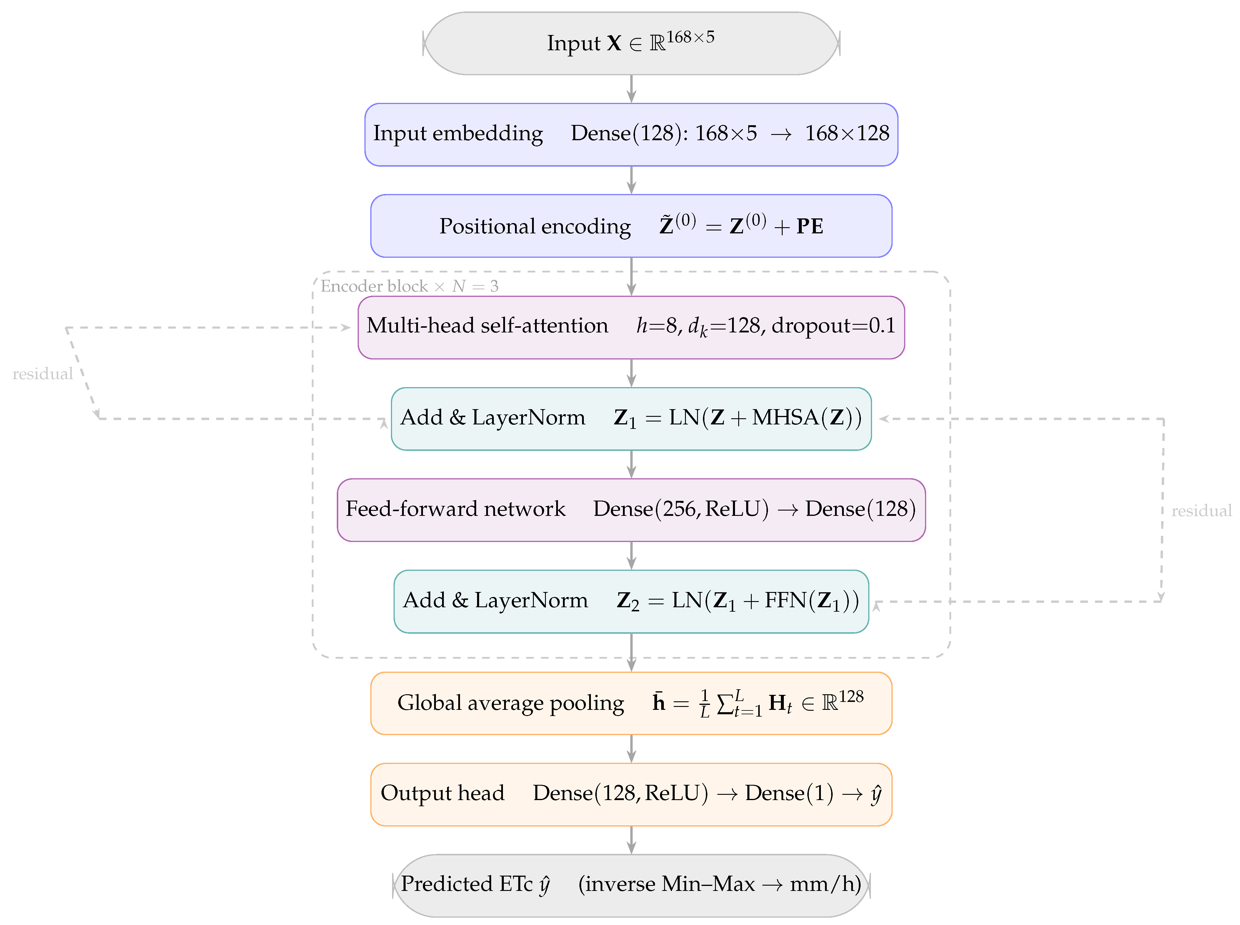
The proposed Transformer encoder model processes a multivariate time-series input $\mathbf{X}\in {\mathbb{R}}^{L\times F}$ ($L=168$, $F=5$) and produces a scalar ETc prediction $\widehat{y}$. The architecture consists of five sequential stages: (1) input embedding, (2) positional encoding, (3) $N=3$ stacked encoder blocks each containing a Multi-Head Self-Attention (MHSA) sub-layer and a position-wise Feed-Forward Network (FFN), both wrapped in residual connections and Layer Normalization, (4) Global Average Pooling, and (5) a fully connected output head [16]. The complete data flow is illustrated in Figure 1.

The architecture, illustrated in Figure 1, consists of five sequential components: (1) a fully connected input embedding that projects each timestep into a $d_{\mathrm{model}}=128$ dimensional space; (2) fixed sinusoidal positional encodings added element-wise to inject temporal order information [16]; (3) $N=3$ stacked encoder blocks, each comprising a Multi-Head Self-Attention (MHSA) sub-layer ($h=8$ heads, $d_k=16$, dropout $p=0.1$) and a position-wise Feed-Forward Network (FFN; Dense (256, ReLU) → Dense (128)), both wrapped in residual connections [31] and Layer Normalization [32,33]; (4) Global Average Pooling (GAP) that reduces the sequence of L hidden vectors to a single fixed-length representation [34,35]; and (5) a two-layer output head (Dense (128, ReLU) → Dense (1)) that produces the scalar ETc prediction, subsequently recovered to mm ${\mathrm{h}}^{-1}$ via inverse Min–Max scaling.

Within each encoder block, residual connections and Layer Normalization are applied sequentially after each sub-layer:

$$\mathbf{z}=\mathrm{LayerNorm}\left(\mathbf{x}+\mathrm{MHSA}\left(\mathbf{x}\right)\right),\mathbf{h}=\mathrm{LayerNorm}\left(\mathbf{z}+\mathrm{FFN}\left(\mathbf{z}\right)\right),$$

(2)

where $\mathbf{x}$, $\mathbf{z}$, $\mathbf{h}\in {\mathbb{R}}^{L\times d_{\mathrm{model}}}$ are the sub-layer input, post-MHSA output, and final block output, respectively. All remaining components follow the standard formulation of Vaswani et al. [16]. A summary of all hyperparameters is provided in

Table 1. Hyperparameter configuration of the proposed Transformer model.

Hyperparameter	Symbol/Notation	Value
Look-back window	L	168 h
Number of input features	F	5
Model dimensionality	$d_{\mathrm{model}}$	128
Number of encoder blocks	N	3
Number of attention heads	h	8
Key/query dimension per head	$d_k$	16
FFN inner dimensionality	$d_{\mathrm{ff}}$	256
Attention dropout rate	p	0.1
Output dense units	—	128
Optimizer	—	Adam
Learning rate	$\eta$	${10}^{-3}$
Batch size	—	32
Maximum epochs	—	60
Early stopping patience	—	10

.

2.5.3. Training Objective

The model was trained by minimizing the Mean Squared Error (MSE) loss over all training samples:

$${\mathcal{L}}_{\mathrm{MSE}}={\displaystyle \frac{1}{N_{\mathrm{train}}}}{\displaystyle \sum _{i=1}^{N_{\mathrm{train}}}}{\left({\widehat{y}}_i-y_i\right)}^2,$$

(3)

where $N_{\mathrm{train}}$ is the number of training samples. Parameters were optimized using the Adam optimizer [36] with a learning rate of $\eta ={10}^{-3}$ and default momentum coefficients ${\beta }_1=0.9$, ${\beta }_2=0.999$. Training was conducted for a maximum of 60 epochs with a mini-batch size of 32. The internal validation subset comprising the last 20% of the training pool was used for early stopping only. Early stopping with a patience of 10 epochs and restoration of the best-validation-loss weights was applied to prevent overfitting [30]. A summary of all Transformer hyperparameters is provided in Table 1.

2.5.4. Dataset Partitioning and Validation Strategy

The complete dataset was partitioned chronologically before any sliding-window construction or scaling was applied. The final 168 h were reserved as the held-out test set, and the remaining observations were divided into training (80%) and internal validation (20%) subsets in strict temporal order, such that all training observations precede all validation observations in calendar time.

Sliding-window samples were subsequently constructed separately within each subset. Near the training–validation split boundary, adjacent windows share overlapping input content of up to $L-1=167$ timesteps, an inherent consequence of applying a sliding-window construction to a continuous time series [29,30]. Critically, this overlap affects only the input window content and does not constitute leakage of future target values, as the target $y_t$ for each sample is always the ETc value at the timestep immediately following the end of its input window, which lies strictly in the future relative to that window’s training data.

It is nonetheless acknowledged that this overlap may cause validation loss near the split boundary to be marginally optimistic as a measure of generalization, since the model may have encountered similar input contexts during training. An embargo gap of $L-1=167$ h between the training and validation subsets was not implemented for the following reasons. First, the internal validation subset is used exclusively for early stopping and is not involved in any reported performance metric; the practical consequence of the overlap is therefore confined to the early stopping criterion and does not affect the integrity of the held-out test set evaluation. Second, imposing a 167-h embargo would remove approximately 0.5% of the total dataset from the validation pool, reducing the number of samples available to monitor convergence without a commensurate benefit given the sole use of the validation subset for early stopping. The acknowledged consequence of not using an embargo gap is that the early stopping criterion may trigger at a marginally suboptimal epoch relative to what a gap-protected criterion would select. However, the training and validation losses converged closely at the optimal checkpoint (0.0016 and 0.0017, respectively) with no sign of overfitting, suggesting that the impact on the selected weights is minimal. All reported performance metrics are computed on the held-out test set only, which remains completely disjoint from both training and validation subsets in calendar time. Implementation of an embargo gap equal to $L-1$ h is identified as a recommended practice for future work [29,30].

The internal validation subset was not used for hyperparameter selection, model comparison, or performance reporting. All reported performance metrics were computed on the held-out test set only, which is completely disjoint from both training and validation subsets in calendar time. The three-way temporal partitioning of the data is summarized in

Table 2. Chronological data partitioning used in this study.

Subset	Duration (Hours)	Samples (Windows)	Purpose
Train subset	≈29,154	≈28,986	Weight update
Val subset	≈7238	≈7070	Early stopping only
Test set	168	168	Performance evaluation
Total	$36,528$	—	—

Val subset = last 20% of raw observations after removing the test set, partitioned chronologically before sliding-window construction. The test set was never used during training or early stopping. Window size $L=168$ h for all subsets.

.

It is acknowledged that evaluation on a single chronological hold-out of 168 h constitutes a limited basis for assessing model generalizability across seasonal variation and diverse meteorological conditions, and this is identified as a boundary of the present contribution.

2.6. Future Forecasting

To demonstrate the model’s potential utility in operational settings, a recursive multi-step forecasting heuristic simulation was implemented. It is emphasized that this exercise is a proof-of-concept demonstration rather than a fully operational forecast because future exogenous meteorological features (temperature, humidity, solar radiation, wind speed) are not available and must be approximated.

Specifically, future exogenous feature values were approximated by copying the corresponding observed values from 72 h prior (equivalent to the same hour three days previously). This replication strategy preserves the diurnal cycle structure but does not account for day-to-day meteorological variability. It therefore does not constitute forecasting without future meteorological information in a realistic operational sense. Only the ETc slot in each new input row was replaced by the model’s own prediction from the previous step.

2.7. Evaluation Metrics

Model performance on the 168-h test set was assessed using six complementary metrics. The first two provide overall measures of predictive accuracy:

$$\mathrm{RMSE}=\sqrt{{\displaystyle \frac{1}{n}}\sum _{t=1}^n{\left({\widehat{y}}_t-y_t\right)}^2}$$

(4)

$$R^2=1-{\displaystyle \frac{{\sum }_{t=1}^n{({\widehat{y}}_t-y_t)}^2}{{\sum }_{t=1}^n{(y_t-\overline{y})}^2}}$$

(5)

The third metric is Mean Absolute Error (MAE):

$$\mathrm{MAE}={\displaystyle \frac{1}{n}}{\displaystyle \sum _{t=1}^n}\left|{\widehat{y}}_t-y_t\right|$$

(6)

Since RMSE and $R^2$ computed over the full hourly cycle may disproportionately reward models that accurately reproduce near-zero nocturnal ETc values, three additional irrigation-relevant metrics were computed to better capture model performance during agronomically critical periods [6].

The fourth metric is the daytime-only RMSE (${\mathrm{RMSE}}_{\mathrm{day}}$), computed exclusively over hours 06:00–18:00 h, when ETc is non-zero and irrigation decisions are most consequential:

$${\mathrm{RMSE}}_{\mathrm{day}}=\sqrt{{\displaystyle \frac{1}{n_d}}\sum _{t\in \mathcal{D}}{\left({\widehat{y}}_t-y_t\right)}^2}$$

(7)

where $\mathcal{D}$ denotes the set of daytime timesteps (06:00–18:00 h) and $n_d=\left|\mathcal{D}\right|$.

The fifth metric is the mean daily peak ETc bias, defined as the mean difference between the predicted and observed daily maximum ETc:

$$\mathrm{Peak}\mathrm{bias}={\displaystyle \frac{1}{D}}{\displaystyle \sum _{d=1}^D}\left(\underset{t\in d}{max}{\widehat{y}}_t-\underset{t\in d}{max}{y}_t\right)$$

(8)

where $D=7$ is the number of forecast days. Negative values indicate systematic underestimation of daily ETc peaks.

The sixth metric is the daily cumulative ETc MAE, which measures the mean absolute error of total predicted ETc per day (mm/day):

$$\mathrm{Daily}\mathrm{MAE}={\displaystyle \frac{1}{D}}{\displaystyle \sum _{d=1}^D}\left|\sum _{t\in d}{\widehat{y}}_t-\sum _{t\in d}{y}_t\right|$$

(9)

where $y_t$ is the observed ETc, ${\widehat{y}}_t$ is the predicted value, $\overline{y}$ is the mean of observed values, and $n=168$. Lower RMSE, MAE, ${\mathrm{RMSE}}_{\mathrm{day}}$, and Daily MAE indicate better predictive accuracy. For Peak bias, values closer to zero indicate less systematic error in peak ETc estimation. For the SARIMA model, in-sample fitted values on the training set were additionally evaluated to characterize goodness-of-fit.

2.8. Software and Reproducibility

All analyses were performed in Python 3.12. The SARIMA model was implemented using the statsmodels 0.14 library [37]. The Transformer model was built with TensorFlow/Keras 2.x. Data preprocessing and evaluation used pandas, NumPy, and scikit-learn [38]. Experiments were conducted on Google Colaboratory (NVIDIA T4 GPU). The complete dataset is publicly available at https://weather-31ba2.web.app/home. The complete source code is available from the corresponding author upon reasonable request.

3. Results

3.1. Model Training

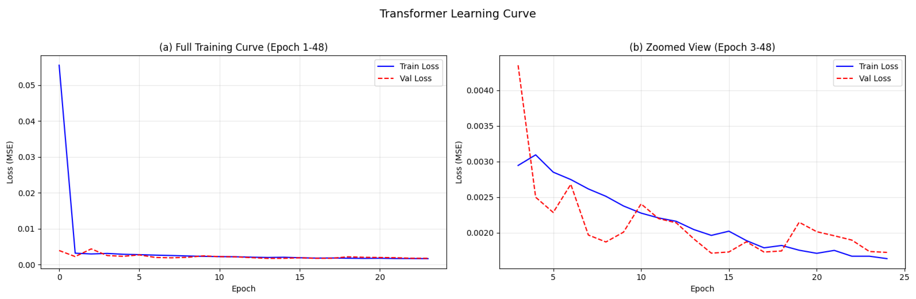
The Transformer model was trained for 24 epochs before early stopping was triggered, indicating that validation loss ceased to improve within the allotted patience of 10 epochs. The best model weights were restored from epoch 14.

The training loss decreased rapidly during the first two epochs, from approximately 0.0555 to 0.0032, and continued to decline gradually thereafter, converging at a training loss of 0.0016 and a validation loss of 0.0017 at the optimal checkpoint. No signs of severe overfitting were observed, as the training and validation losses remained closely aligned throughout the training process (Figure 2). These results confirm that the early stopping strategy with best-weight restoration was effective in obtaining a well-generalized model.

3.2. Stationarity Analysis

Prior to model comparison, the Augmented Dickey–Fuller (ADF) test was applied to the ETc time series to verify stationarity. The results are summarized in

Table 3. Augmented Dickey–Fuller (ADF) test results for the ETc time series.

Series	ADF Statistic	p-Value	Conclusion
ETc (original)	$-13.063$	$2.03\times {10}^{-24}$	Stationary
ETc (1st differencing)	$-40.054$	<0.001	Stationary

Critical values at 1%, 5%, and 10% significance levels are $-3.431$, $-2.862$, and $-2.567$, respectively. Number of observations used: 36,475; lags selected by AIC: 52.

. The original ETc series yielded an ADF statistic of $-13.06$ with a p-value of $2.03\times {10}^{-24}$, well below the 1% significance threshold ($-3.431$), providing strong evidence against the null hypothesis of a unit root. Consequently, the series is stationary in its original form, which is consistent with the SARIMA model specification using $d=1$ purely for capturing autoregressive dynamics rather than for removing a stochastic trend. First-order differencing further reduced the ADF statistic to $-40.05$ ($p\approx 0$), confirming robust stationarity.

3.3. ETc Estimation Performance on the Test Set

Table 4. ETc estimation performance comparison on the 168-h test set.

Model	RMSE	MAE	${\mathit{R}}^2$	RMSEday	Peak Bias	Daily MAE
SARIMA$(2,1,2){(1,0,0)}_{24}$	0.0717	0.0593	0.4688	0.0791	−0.0965	0.5901
Transformer	0.0308	0.0188	0.9018	0.0414	−0.0180	0.1599
Improvement	$\downarrow 57.0\%$	$\downarrow 68.3\%$	$\uparrow 92.4\%$	$\downarrow 47.7\%$	—	$\downarrow 72.9\%$

Bold values indicate the best-performing model. RMSE and MAE are computed in the original ETc scale (mm/h). RMSE_day: daytime-only RMSE (06:00–18:00 h). Peak bias: mean daily peak ETc bias (mm/h); negative values indicate underestimation. Daily MAE: mean absolute error of daily cumulative ETc (mm/day). $R^2$: coefficient of determination; higher is better (maximum 1.0). ↓: percentage reduction relative to SARIMA; ↑: percentage improvement relative to SARIMA.

presents the ETc estimation performance of the SARIMA baseline and the proposed Transformer model evaluated on the 168-h test set across six complementary metrics. The Transformer model achieved an RMSE of 0.0308 mm/h, MAE of 0.0188 mm/h, and $R^2$ of 0.9018, substantially outperforming SARIMA (RMSE = 0.0717, MAE = 0.0593, $R^2$ = 0.4688). The Transformer’s RMSE was approximately 57% lower than that of SARIMA, while its $R^2$ was approximately 0.43 units higher, indicating that the model explained over 90% of the variance in the observed ETc values during the test period.

It is noted at the outset that this evaluation is based on a single 168-h test episode, without multivariate statistical baselines such as SARIMAX with exogenous inputs or machine learning comparators; the absence of these baselines means that the observed performance gap cannot be attributed solely to the Transformer architecture.

The Transformer outperformed SARIMA on all reported metrics. Three design differences between the two models may contribute to this gap: the Transformer’s multivariate input design incorporating four meteorological features, its 168-h self-attention window enabling direct comparison of any two timesteps within the look-back period, and its three stacked encoder blocks. However, the current experimental design does not isolate these factors, as the Transformer differs from SARIMA simultaneously in input dimensionality, model architecture, and temporal dependency structure. It is therefore not possible to determine from the present results whether the performance gains are attributable to the self-attention architecture, the multivariate input design, or the combination of both. A comparison with a multivariate statistical baseline such as SARIMAX would be required to isolate these contributions and is identified as a direction for future research.

The irrigation-relevant metrics provide evaluation criteria that are more consistent with agronomic contexts than hourly RMSE alone. However, they remain statistical proxies rather than demonstrated irrigation outcomes. The daytime-only RMSE (${\mathrm{RMSE}}_{\mathrm{day}}$) was 0.0414 mm/h for the Transformer versus 0.0791 mm/h for SARIMA, representing a 47.7% reduction, indicating more accurate reproduction of ETc during daytime hours, a period that is agronomically relevant for irrigation scheduling, though the present study does not evaluate actual irrigation decisions or outcomes.

The mean daily peak ETc bias was −0.0180 mm/h for the Transformer and −0.0965 mm/h for SARIMA. Both models exhibited a tendency to underestimate daily peak ETc values, but the magnitude of underestimation was substantially smaller for the Transformer, indicating more accurate reproduction of maximum daily water demand.

The daily cumulative ETc MAE was 0.1599 mm/day for the Transformer versus 0.5901 mm/day for SARIMA, a 72.9% reduction, reflecting more accurate statistical proxies of total daily water demand. These metrics are more consistent with irrigation-relevant evaluation criteria than hourly RMSE alone, but do not constitute demonstrated field-scale irrigation outcomes.

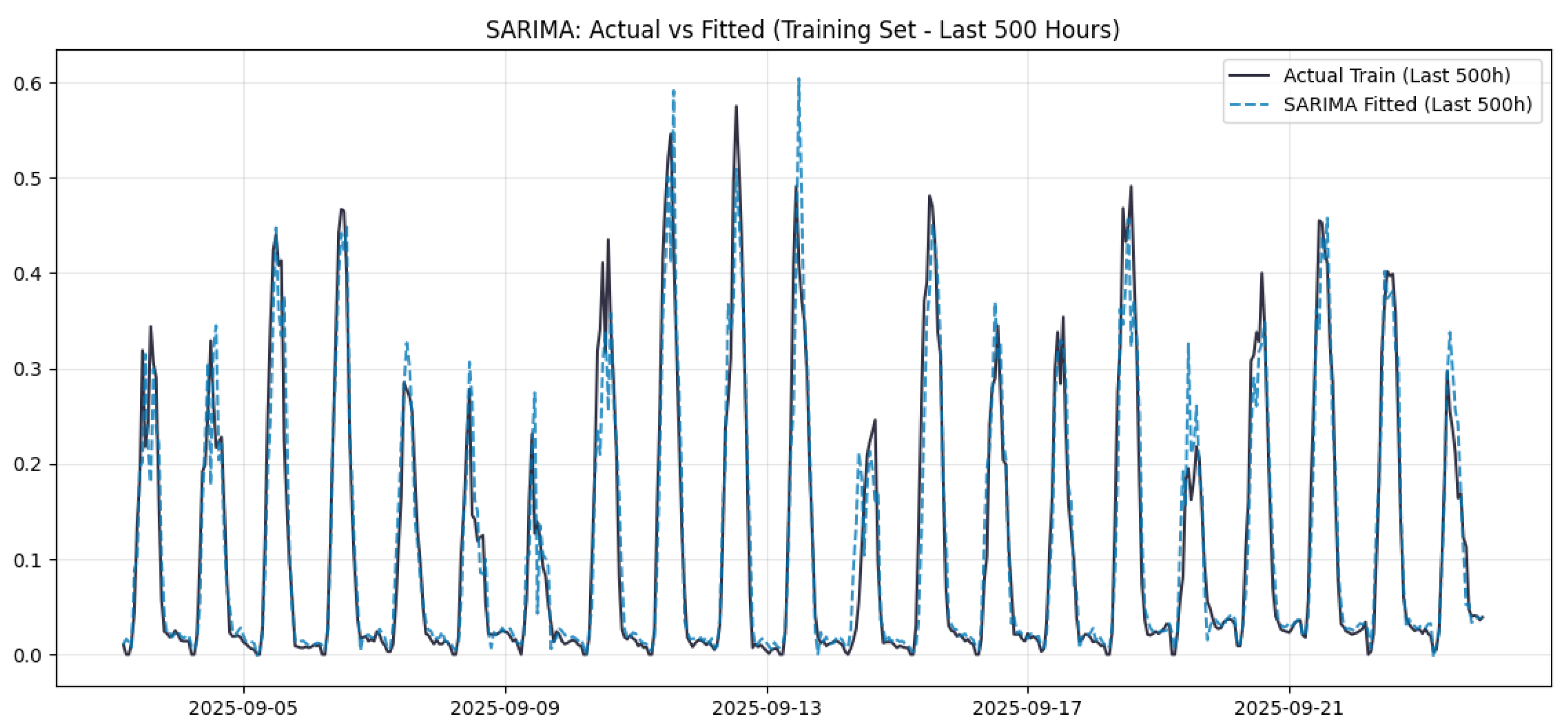
The in-sample performance of the SARIMA model on the training set is illustrated in Figure 3. The fitted values closely follow the observed diurnal pattern over the last 500 h of the training period, achieving a training RMSE of 0.0392 and $R^2$ of 0.9539, indicating that the model captured the general seasonal structure of the ETc series during fitting. However, the considerably lower test-set performance (RMSE = 0.0717, $R^2$ = 0.4688) suggests limited generalization to unseen data, particularly during periods of anomalous solar radiation and atypical meteorological conditions. Note that Figure 3 covers the training period (4–23 September 2025), while Figure 4 covers the held-out test period (24 September–1 October 2025); the two figures necessarily cover different time windows because they serve different analytical purposes.

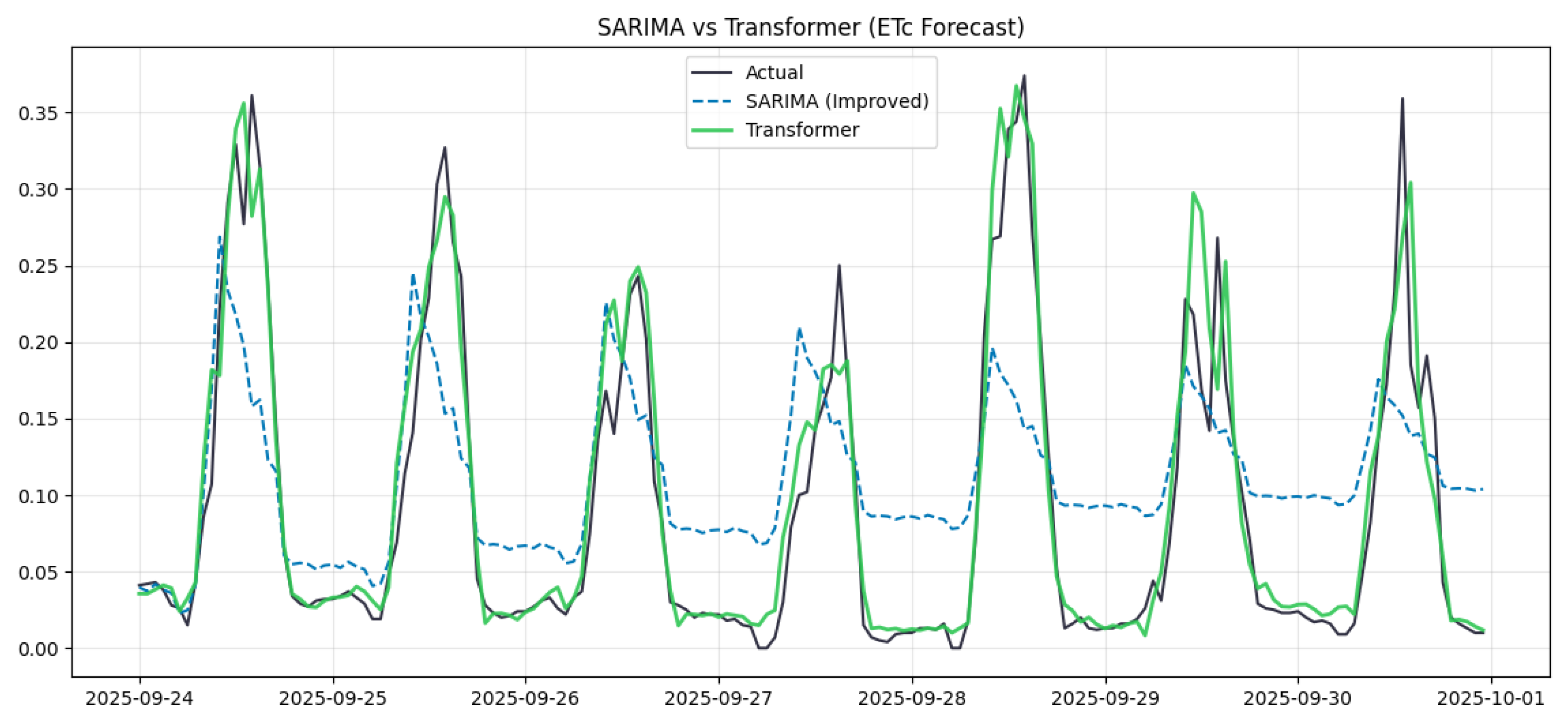
Figure 4 provides a visual illustration of the qualitative difference in forecasting behavior between the two models over the selected test week. The Transformer more closely tracks the diurnal fluctuations of the observed series, whereas the SARIMA forecast exhibits a damped amplitude response and underestimates the magnitude of daytime ETc peaks during high-radiation periods. It should be noted, however, that this figure represents a single 168-h test episode and is intended to illustrate qualitative differences in model behavior rather than serve as evidence of general predictive superiority. Performance over other seasonal periods or meteorological conditions may differ, and rolling-origin evaluation across multiple non-overlapping test windows is identified as an important direction for future research.

The test period (24 September–1 October 2025) falls within Thailand’s rainy season, which is characterized by higher cloud cover, reduced solar radiation, and lower ETc peaks relative to the dry season (November–April). The representativeness of this test week with respect to the full four-year dataset—which spans both rainy and dry season conditions—has not been formally established. Model performance during dry season periods, which typically exhibit higher solar radiation and substantially higher ETc peaks, remains untested. The visual comparison in Figure 4 should therefore be interpreted as an illustration of qualitative model behavior under rainy season conditions only, not as evidence of performance across diverse seasonal contexts.

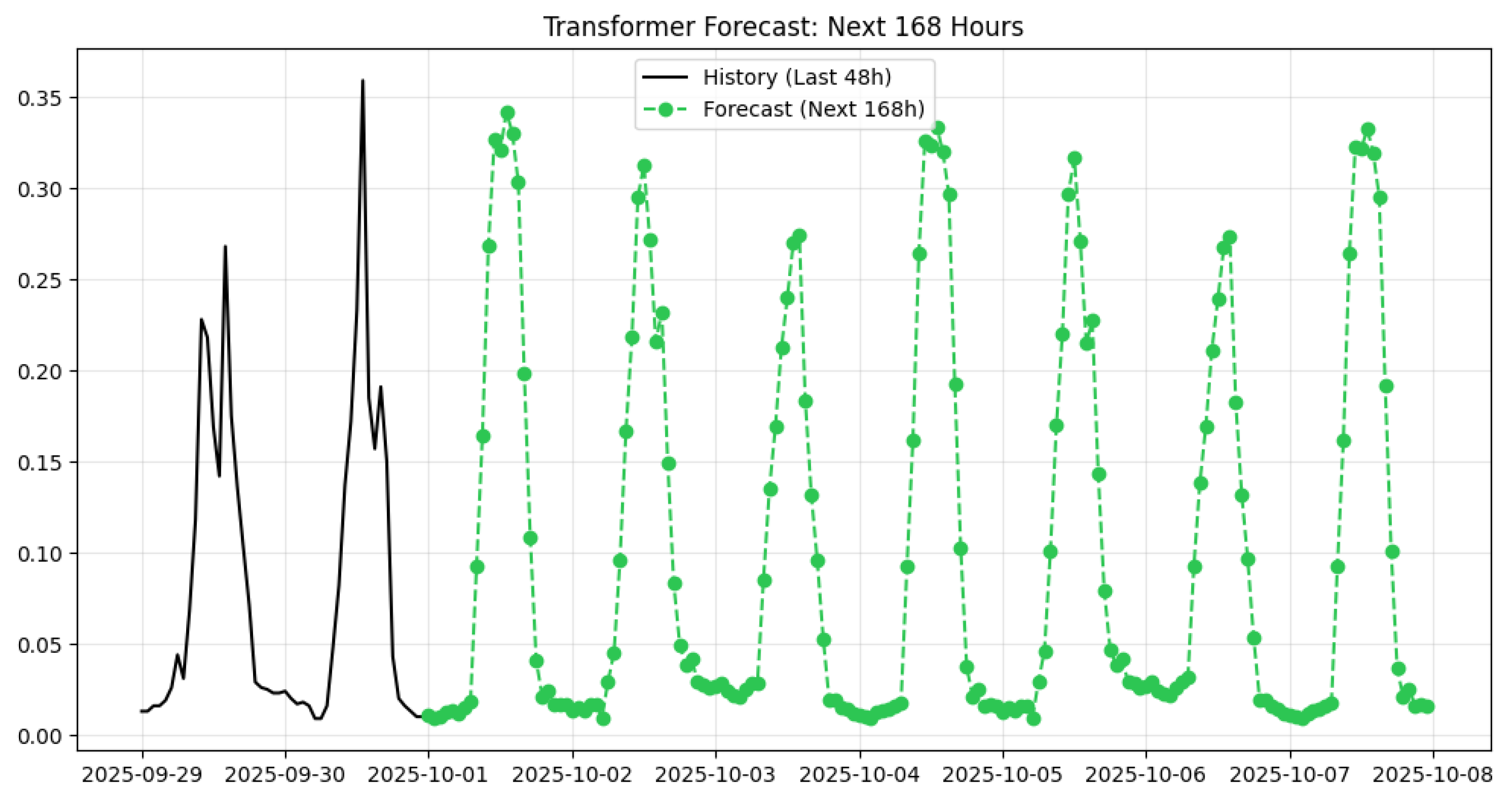
3.4. Future Forecasting

To demonstrate the model’s potential utility in a proof-of-concept setting, the trained Transformer was deployed in a recursive multi-step heuristic simulation to predict ETc for the subsequent 168 h beyond the end of the available record (Figure 5). At each step, the model predicted one hour ahead; the forecast window was then advanced by one timestep, and the predicted ETc value was inserted into the input sequence. Exogenous feature values (temperature, humidity, solar radiation, and wind speed) for future timesteps were approximated using the corresponding observations from 72 h prior (equivalent to the same hour three days previously). This replication strategy preserves the diurnal cycle structure of the meteorological inputs but does not represent real future meteorological uncertainty, as day-to-day variability in temperature, humidity, solar radiation, and wind speed is not captured. The exercise should therefore be interpreted solely as a heuristic simulation demonstrating that the model can generate physically plausible ETc patterns under a simplified meteorological approximation, and not as evidence of operational multi-step forecasting capability. The 168-h simulation exhibits a physically plausible diurnal pattern, with ETc values rising during daylight hours and approaching zero at night, consistent with the dependence of evapotranspiration on solar radiation. The peak ETc values in the forecast period are comparable in magnitude to those observed in the 168-h history window, suggesting that the 72-h feature replication strategy preserved the general diurnal structure under the approximated meteorological scenario.

Figure 5 presents the recursive 168-h ETc simulation generated by the trained Transformer model for the period 1–8 October 2025, immediately following the end of the available observation record. The black line represents the last 48 h of observed ETc, serving as the historical context window, while the green dashed line with markers shows the model’s predictions for the subsequent 168 h.

The simulation exhibits a physically plausible and consistent diurnal pattern throughout the entire 7-day horizon. ETc values rise sharply during daylight hours, reaching daily peaks of approximately 0.28–0.35 mm/h between late morning and early afternoon, and approach near-zero values during night-time hours, consistent with the dependence of evapotranspiration on incoming solar radiation. The amplitude and timing of predicted diurnal peaks remain stable across all seven forecast days, with no evidence of cumulative error propagation or systematic drift.

These results demonstrate that under the 72-h feature replication heuristic, the model generates physically plausible diurnal ETc patterns across the 7-day simulation horizon. However, this exercise constitutes a heuristic simulation rather than a fully rigorous operational forecast, as the exogenous meteorological inputs are approximated rather than independently predicted. The results should therefore be interpreted as a proof-of-concept demonstration of the model’s ability to maintain physically consistent ETc patterns under an approximated meteorological scenario, rather than as evidence of operational forecasting capability without future weather data.

4. Discussion

4.1. Transformer Performance Relative to SARIMA

The Transformer encoder model substantially outperformed the SARIMA baseline on the 168-h test set, achieving an RMSE of 0.0308 mm/h and $R^2$ of 0.9018 compared with RMSE = 0.0717 and $R^2$ = 0.4688 for SARIMA. These findings are consistent with the broader literature reporting that deep learning models outperform classical statistical approaches for hourly and sub-daily PM-derived ETc estimation, particularly when multiple meteorological drivers are available as inputs [6]. LSTM-based models applied to daily ETc forecasting in tropical conditions have demonstrated strong predictive accuracy relative to physics-based baselines [9,12], while GRU-based approaches for sub-daily ET estimation have shown competitive performance under similar meteorological input configurations [10]. The Transformer encoder proposed in this study achieves competitive accuracy at hourly resolution in a tropical orchard setting, suggesting that self-attention mechanisms offer a viable alternative to recurrent architectures for this estimation task.

It should be noted that these metrics are computed over a single 168-h test period, representing one meteorological episode in late September 2025. While the results are consistent with the broader literature on deep learning versus statistical baselines for ETc estimation, they should be interpreted as site-specific and period-specific findings. A rolling-origin evaluation across multiple non-overlapping test windows spanning different seasons would provide a more robust assessment of generalization performance [39,40].

The comparison between the multivariate Transformer and the univariate SARIMA baseline is structurally unbalanced in three respects: input dimensionality (five meteorological features versus the ETc series alone), temporal context (168-h self-attention window versus autoregressive lags), and model family (nonlinear deep learning versus linear statistical model) [41]. The observed performance gap therefore reflects a combination of these factors and cannot be attributed to the self-attention architecture alone. This is not merely a future direction but a necessary caveat for interpreting the present results: the current design demonstrates that the combined Transformer configuration outperforms a univariate statistical baseline on this dataset and test period, but does not establish which design element drives the improvement. A fair architectural comparison would require at minimum a SARIMAX model with exogenous meteorological inputs, a multivariate machine learning baseline such as XGBoost or Random Forest, and a univariate Transformer operating on the ETc series alone [6,41].

The relatively modest generalization performance of SARIMA ($R^2=0.4688$ on the test set versus $R^2=0.9539$ on the training set) highlights the well-known limitations of univariate linear time-series models when applied to ETc estimation in variable tropical climates. The large gap between in-sample and out-of-sample performance is attributable to two structural constraints: first, SARIMA cannot assimilate concurrent meteorological covariates such as solar radiation and relative humidity, which are the primary drivers of day-to-day ETc variability; second, the fixed seasonal structure assumed by SARIMA$(2,1,2){(1,0,0)}_{24}$ may be inadequate to represent non-stationary ETc dynamics arising from irregular cloud cover and rainfall events common in Chanthaburi Province during the study period [14,26]. These observations are in line with findings by [6], who reported that multivariate machine learning models consistently outperformed univariate statistical baselines for reference ET estimation under data-sparse and climatically variable conditions.

4.2. Role of Multivariate Inputs and Long Look-Back Window

A key distinguishing feature of the proposed model is its use of five concurrent meteorological features and a 168-h (7-day) look-back window. The ETc values used in this study were computed from the same four meteorological inputs (solar radiation, temperature, relative humidity, and wind speed) using the FAO-56 Penman–Monteith equation. The Transformer encoder therefore learns to approximate this functional relationship from sequential meteorological observations, rather than forecasting an independently measured agronomic variable [42,43].

This distinction has important implications for interpreting the high $R^2$ of 0.9018. The strong performance reflects the model’s ability to approximate a deterministic mathematical relationship between inputs and a derived target, not its ability to predict actual crop water use under variable biophysical conditions. Independently measured ETc, obtained from lysimeter or eddy-covariance systems, reflects actual crop water use including stomatal regulation, soil water limitation, and canopy boundary-layer effects not captured by the PM equation [43,44]. Model performance against measured ETc is therefore likely to be lower than against PM-derived ETc, particularly under water stress conditions, partial canopy cover, or periods when the FAO-56 crop coefficient does not accurately represent local crop status. This is not a limitation unique to the present study—it is an inherent consequence of using a PM-derived target and must be acknowledged as a boundary of interpretation rather than deferred as future work [42].

Within this context, the inclusion of all four meteorological drivers as input features is consistent with the physical basis of the FAO-56 PM framework [1], in which ETc is determined by the joint action of radiation, temperature, vapour pressure deficit, and aerodynamic resistance. The 168-h look-back window further enables the model to capture temporal patterns in these drivers, particularly the sharp diurnal rise and fall of solar radiation that dominates hourly ETc fluctuations in tropical orchards [29,30].

The choice of $L=168$ h was motivated by the need to encompass both the 24-h diurnal cycle and the 7-day weekly periodicity of ETc, which have been observed to influence irrigation demand patterns in perennial orchard crops [29,30]. The self-attention mechanism, by directly comparing any two positions within the 168-h window, can in principle capture these periodicities without relying on the sequential state propagation required by LSTM or GRU architectures. However, this interpretation remains inferential. The present study does not include an ablation analysis, a univariate Transformer baseline, or a multivariate statistical comparison such as SARIMAX. It is therefore not possible to determine from the current results whether the performance gains are attributable to the self-attention architecture, the multivariate input design, the 168-h temporal context, or the combination of these factors. The claims in this section should therefore be read as plausible hypotheses consistent with the observed results, rather than as demonstrated causal mechanisms.

The test results show that the Transformer more closely reproduced the timing and amplitude of daytime ETc peaks across all seven test days compared with SARIMA, including days with lower peak ETc values (27–28 September 2025). The lower peaks on these days are consistent with reduced solar radiation input, as solar radiation is the dominant driver of hourly ETc in the FAO-56 PM framework, though the specific meteorological cause cannot be confirmed without additional observational data.

4.3. Operational Applicability of Recursive Forecasting

The heuristic simulation demonstrated that under the 72-h feature replication approximation, the trained model generates physically plausible and stable diurnal ETc patterns across the 7-day simulation horizon, with no evidence of systematic drift or amplitude decay. These results should be interpreted as a proof-of-concept demonstration of the model’s ability to maintain physically consistent ETc patterns under an approximated meteorological scenario, rather than evidence of fully autonomous operational forecasting capability [3,21].

It should be emphasized that the 72-h feature replication strategy is a heuristic approximation that does not constitute forecasting without future meteorological information in a realistic operational sense, as it assumes that meteorological conditions three days prior are representative of future conditions. This assumption may be reasonable during periods of stable weather but is likely to introduce error during periods of sustained meteorological change, such as the onset of the monsoon season or multi-day cloudy spells.

More fundamentally, the recursive simulation does not test the model’s ability to forecast ETc from independently predicted meteorological inputs—it tests only whether the model can maintain physically plausible ETc patterns when fed a simplified approximation of future weather. The two tasks are structurally different: the first requires a coupled meteorological forecasting system, while the second requires only a self-consistent diurnal pattern. The physically plausible output shown in Figure 5 is therefore a necessary but not sufficient condition for operational multi-step ETc forecasting. True operational deployment would require integration with independently forecast meteorological inputs from a numerical weather prediction (NWP) source, replacing the replication heuristic with data-driven atmospheric projections [19,22]. Until such integration is demonstrated and validated against independently measured ETc, the recursive simulation exercise should be understood as a feasibility demonstration rather than a validated forecasting procedure.

4.4. Implications for Smart Irrigation in Tropical Horticulture

The results of this study suggest several potential advantages of the proposed approach for data-driven irrigation management, subject to the limitations noted in this study. These should be understood as directions for future applied research rather than demonstrated operational outcomes.

First, the model relies solely on meteorological variables routinely available from low-cost weather monitoring platforms, without requiring specialised sensors or atmospheric sounding equipment required by the FAO-56 PM method [1,4]. If validated with on-site sensor data and independently measured ETc values, this characteristic could make the approach accessible to smallholder tropical orchards with limited instrumentation infrastructure.

Second, once trained, the model performs inference at low computational cost and could in principle be deployed on edge computing devices or cloud-based platforms. Whether this translates to reliable hourly irrigation decisions at the field scale would depend on the model’s performance under real sensor conditions, which has not been evaluated in the present study.

Third, the model’s 168-h look-back window and one-step-ahead forecasting capability suggest potential utility for supporting advance estimates of crop water demand during critical fruit development and maturation stages of durian [12]. However, the present study evaluated the model only on meteorological data from the Visual Crossing Weather API and did not assess its performance using externally supplied weather forecasts, decision-relevant irrigation metrics, or real management outcomes. Claims about weekly irrigation planning or field-scale optimization therefore remain speculative at this stage.

Establishing the irrigation usefulness of the proposed model would require a structured validation program that goes beyond statistical accuracy metrics on a held-out test set. At minimum, four components would be necessary. First, the model’s ETc estimates would need to be compared against a conventional irrigation scheduling approach, such as FAO-56 PM computed from on-site sensor readings or a standard crop-coefficient calendar, to determine whether model-guided scheduling produces materially different irrigation prescriptions under field conditions [45]. Second, water-use efficiency metrics, including total seasonal irrigation volume and irrigation water productivity, would need to be quantified across model-guided and conventional treatments in a replicated field trial [46]. Third, agronomic outcomes, including durian yield, fruit quality, and physiological indicators of water stress, would need to be assessed to determine whether any reduction in estimated water demand translates to maintained or improved crop performance [3]. Fourth, the model’s robustness under real sensor conditions would need to be evaluated, including its behaviour under sensor noise, calibration drift, and missing data typical of low-cost IoT deployments in tropical orchard environments [21]. None of these components has been addressed in the present study, and claims about irrigation benefit therefore remain speculative pending such field-based validation.

It is also worth noting that even if the model performs well against PM-derived ETc under API-sourced meteorological inputs, additional uncertainty would arise when transitioning to on-site IoT sensor data. API-sourced gridded estimates may differ systematically from in situ measurements due to topographic and microclimate effects specific to the orchard canopy environment. The performance gap between API-sourced and sensor-sourced inputs has not been evaluated in the present study and represents an additional validation step required before operational deployment [21,22].

4.5. Limitations and Future Research Directions

Several limitations of the present study should be acknowledged. First, the meteorological data used in this study were obtained from the Visual Crossing Weather API for the orchard location in Chanthaburi Province, rather than from on-site IoT sensors installed directly in the orchard. Throughout this study, ETc refers exclusively to values computed via the FAO-56 Penman–Monteith equation from API-retrieved meteorological inputs, not to independently measured field evapotranspiration [42,44]. Accordingly, the model learns to approximate a deterministic mathematical relationship between meteorological variables and ETc, rather than forecasting an independently measured agronomic variable. Field validation using direct on-site sensor measurements and independently observed ETc values remains an essential next step before operational deployment.

Second, the model was trained and evaluated on data representing a single orchard location in Chanthaburi Province. Its generalizability to other durian-growing regions or different crop types has not been established. Transfer learning or domain adaptation strategies may be required to extend the model to new sites with limited historical data.

Third, the train–test split comprised a single chronological hold-out period of 168 h, representing less than 0.5% of the total dataset. While this design preserves temporal integrity and avoids data leakage, a rolling-window cross-validation scheme over multiple test periods would provide a more robust estimate of out-of-sample performance and model generalization across different seasons and meteorological conditions [39,40]. It is noted, however, that the training pool comprised approximately 36,192 sliding-window samples spanning four years of continuous hourly observations, which is considered sufficient for training the Transformer architecture employed in this study.

Several directions are identified for future research. First, validation using data from on-site IoT sensors together with independently measured ETc from lysimeter or eddy-covariance systems would confirm whether the model’s performance holds under real field conditions with sensor noise and data gaps. Second, incorporating additional input features, including vapor pressure deficit [47], soil moisture from multi-source remote sensing [48], and land surface temperature [49], would enrich the model’s representation of crop water demand. Third, a systematic comparison with SARIMAX, Random Forest, and state-of-the-art architectures such as Informer [19] and TimesNet under identical experimental conditions would clarify the relative contribution of multivariate inputs versus architectural design. Fourth, replacing the 72-h replication heuristic with NWP outputs would substantially improve the operational relevance of the multi-step ETc simulation [19]. Fifth, integrating the model into a closed-loop automated irrigation controller and evaluating it against agronomic benchmarks in a replicated field trial represents essential steps toward practical deployment. Sixth, rolling-origin evaluation across multiple seasonal test periods, together with a formal sensitivity analysis of individual input features, would provide stronger evidence of model generalizability [39].

5. Conclusions

This study developed and evaluated a Transformer encoder model for one-step-ahead hourly FAO-56 PM-derived crop evapotranspiration (ETc) estimation in a durian orchard in Chanthaburi Province, Eastern Thailand. Meteorological data were obtained from the Visual Crossing Weather API for the orchard location over four years, with ETc computed using the FAO–56 Penman-Monteith equation. The model was benchmarked against a SARIMA$(2,1,2){(1,0,0)}_{24}$ statistical baseline under identical data partitioning conditions.

On the 168-h held-out test set, the Transformer achieved an RMSE of 0.0308 mm/h, MAE of 0.0188 mm/h, and $R^2$ of 0.9018, compared with RMSE = 0.0717, MAE = 0.0593, and $R^2$ = 0.4688 for SARIMA, representing a 57.0% reduction in RMSE, a 68.3% reduction in MAE, and a 92.4% improvement in $R^2$. Three design differences between the models—multivariate meteorological inputs, the 168-h self-attention window, and stacked encoder blocks—may contribute to this performance gap, though the present study does not isolate these factors, and the gains cannot be causally attributed to any single design choice.

A recursive 168-h heuristic simulation showed that the model generates physically plausible diurnal ETc patterns under a 72-h feature replication approximation. This exercise is a proof-of-concept demonstration rather than a rigorous operational forecast, as future meteorological inputs were approximated rather than independently predicted.

The study is best understood as a site-specific proof of concept. It demonstrates that a Transformer encoder can learn to approximate the FAO-56 PM functional relationship from sequential meteorological observations at hourly resolution and that the resulting model outperforms a SARIMA baseline on a single test episode at one orchard location. These results are encouraging but cannot be generalized to other sites, crop types, or seasons without further validation. Future work should prioritize field validation using on-site sensor data and independently measured ETc, ablation analysis to isolate the contribution of individual design choices, comparison with multivariate baselines such as SARIMAX, rolling-origin evaluation across multiple seasonal test periods, and integration with numerical weather prediction outputs for operationally rigorous multi-step forecasting.

References

1. Wanniarachchi, S.; Sarukkalige, R. A review on evapotranspiration estimation in agricultural water management: Past, present, and future. Hydrology 2022, 9, 123. [Google Scholar] [CrossRef]
2. Sarker, K.K.; Karim, N.N.; Islam, A.T.; Ahmed, I.; Uddin, M.N.; Hasan, S.; Hoque, M.R.; Ali, M.T.; Kabir, M.S.; Biswas, S.K.; et al. Field evaluation of sensor-driven drip irrigation systems for eggplant production. BMC Agric. 2026, 2, 7. [Google Scholar] [CrossRef]
3. Bwambale, E.; Abagale, F.K.; Anornu, G.K. Data-driven model predictive control for precision irrigation management. Smart Agric. Technol. 2023, 3, 100074. [Google Scholar] [CrossRef]
4. Sentelhas, P.C.; Gillespie, T.J.; Santos, E.A. Evaluation of FAO Penman–Monteith and alternative methods for estimating reference evapotranspiration with missing data in Southern Ontario, Canada. Agric. Water Manag. 2010, 97, 635–644. [Google Scholar] [CrossRef]
5. Jagtap, S.S.; Chan, A.K. Agrometeorological aspects of agriculture in the sub-humid and humid zones of Africa and Asia. Agric. For. Meteorol. 2000, 103, 59–72. [Google Scholar] [CrossRef]
6. Taheri, M.; Bigdeli, M.; Imanian, H.; Mohammadian, A. An overview of evapotranspiration estimation models utilizing artificial intelligence. Water 2025, 17, 1384. [Google Scholar] [CrossRef]
7. Just, A.C.; Arfer, K.B.; Rush, J.; Dorman, M.; Shtein, A.; Lyapustin, A.; Kloog, I. Advancing methodologies for applying machine learning and evaluating spatiotemporal models of fine particulate matter (PM2.5) using satellite data over large regions. Atmos. Environ. 2020, 239, 117649. [Google Scholar] [CrossRef]
8. Xu, Y.; Ho, H.C.; Wong, M.S.; Deng, C.; Shi, Y.; Chan, T.C.; Knudby, A. Evaluation of machine learning techniques with multiple remote sensing datasets in estimating monthly concentrations of ground-level PM2.5. Environ. Pollut. 2018, 242, 1417–1426. [Google Scholar] [CrossRef]
9. ArunKumar, K.; Kalaga, D.V.; Kumar, C.M.S.; Kawaji, M.; Brenza, T.M. Comparative analysis of Gated Recurrent Units (GRU), long Short-Term memory (LSTM) cells, autoregressive Integrated moving average (ARIMA), seasonal autoregressive Integrated moving average (SARIMA) for forecasting COVID-19 trends. Alex. Eng. J. 2022, 61, 7585–7603. [Google Scholar] [CrossRef]
10. Sajjad, M.; Khan, Z.A.; Ullah, A.; Hussain, T.; Ullah, W.; Lee, M.Y.; Baik, S.W. A novel CNN-GRU-based hybrid approach for short-term residential load forecasting. IEEE Access 2020, 8, 143759–143768. [Google Scholar] [CrossRef]
11. Michael, N.E.; Bansal, R.C.; Ismail, A.A.A.; Elnady, A.; Hasan, S. A cohesive structure of Bi-directional long-short-term memory (BiLSTM)-GRU for predicting hourly solar radiation. Renew. Energy 2024, 222, 119943. [Google Scholar] [CrossRef]
12. Thongnim, P.; Inthasuth, T.; Leelaphaiboon, M. Integrating LSTM-based VPD forecasting into IoT-driven smart irrigation systems in tropical orchards. Discov. Sustain. 2025, 7, 173. [Google Scholar] [CrossRef]
13. Jackson, C.; Preston, N.; Thompson, P.J.; Burford, M. Nitrogen budget and effluent nitrogen components at an intensive shrimp farm. Aquaculture 2003, 218, 397–411. [Google Scholar] [CrossRef]
14. Alharbi, F.R.; Csala, D. A seasonal autoregressive integrated moving average with exogenous factors (SARIMAX) forecasting model-based time series approach. Inventions 2022, 7, 94. [Google Scholar] [CrossRef]
15. Liu, H.; Li, C.; Shao, Y.; Zhang, X.; Zhai, Z.; Wang, X.; Qi, X.; Wang, J.; Hao, Y.; Wu, Q.; et al. Forecast of the trend in incidence of acute hemorrhagic conjunctivitis in China from 2011–2019 using the Seasonal Autoregressive Integrated Moving Average (SARIMA) and Exponential Smoothing (ETS) models. J. Infect. Public Health 2020, 13, 287–294. [Google Scholar] [CrossRef] [PubMed]
16. Vaswani, A.; Shazeer, N.; Parmar, N.; Uszkoreit, J.; Jones, L.; Gomez, A.N.; Kaiser, Ł.; Polosukhin, I. Attention is all you need. Adv. Neural Inf. Process. Syst. 2017, 30, 1–11. [Google Scholar]
17. Tie, R.; Li, M.; Zhou, C.; Ding, N. Research on the application of an improved Autoformer model integrating CNN-attention-BiGRU in short-term power load forecasting. Evol. Syst. 2025, 16, 98. [Google Scholar] [CrossRef]
18. Zhu, Y.; Pu, L.; Yang, D.; Kang, T.; Liang, C.; Peng, M.; Zhai, C. A Virtual Power Plant Load Forecasting Approach Using COM Encoding and BiLSTM-Att-KAN. Energies 2025, 18, 5598. [Google Scholar] [CrossRef]
19. Ampas, H.; Refanidis, I.; Ampas, V. Hybrid hydrological forecasting through a physical model and a weather-informed transformer model: A case study in Greek watershed. Appl. Sci. 2025, 15, 6679. [Google Scholar] [CrossRef]
20. Song, Z.; Tsang, H.S.H.; Hsung, R.T.C.; Zhu, Y.; Lo, W.L. From Market Volatility to Predictive Insight: An Adaptive Transformer–RL Framework for Sentiment-Driven Financial Time-Series Forecasting. Forecasting 2025, 7, 55. [Google Scholar] [CrossRef]
21. Zanella, A.; Zubelzu, S.; Bennis, M. Sensor networks, data processing, and inference: The hydrology challenge. IEEE Access 2023, 11, 107823–107842. [Google Scholar] [CrossRef]
22. de Chalendar, J.A.; McMahon, C.; Valenzuela, L.F.; Glynn, P.W.; Benson, S.M. Unlocking demand response in commercial buildings: Empirical response of commercial buildings to daily cooling set point adjustments. Energy Build. 2023, 278, 112599. [Google Scholar] [CrossRef]
23. Sinsomboonthong, S. Performance comparison of new adjusted min-max with decimal scaling and statistical column normalization methods for artificial neural network classification. Int. J. Math. Math. Sci. 2022, 2022, 3584406. [Google Scholar] [CrossRef]
24. Ivanovski, Z.; Ivanovska, N. The augmented dickey-fuller test for the stationarity of the final public consumption and gdp time series of the republic of north macedonia. UTMS J. Econ. 2024, 15, 109–124. [Google Scholar]
25. Roza, A.; Violita, E.S.; Aktivani, S. Study of inflation using stationary test with augmented dickey fuller & phillips-peron unit root test (Case in bukittinggi city inflation for 2014–2019). EKSAKTA Berk. Ilm. Bid. MIPA 2022, 23, 106–116. [Google Scholar] [CrossRef]
26. Szostek, K.; Mazur, D.; Drałus, G.; Kusznier, J. Analysis of the effectiveness of ARIMA, SARIMA, and SVR models in time series forecasting: A case study of wind farm energy production. Energies 2024, 17, 4803. [Google Scholar] [CrossRef]
27. Box, G. Box and Jenkins: Time series analysis, forecasting and control. In A Very British Affair: Six Britons and the Development of Time Series Analysis During the 20th Century; Springer: Berlin/Heidelberg, Germany, 2013; pp. 161–215. [Google Scholar]
28. Broersen, P.; De Waele, S. Empirical time series analysis and maximum likelihood estimation. In Proceedings of the IEEE Benelux Signal Processing Symposium; IEEE: New York, NY, USA, 2000; pp. 1–4. [Google Scholar]
29. Lim, B.; Zohren, S. Time-series forecasting with deep learning: A survey. Philos. Trans. R. Soc. A Math. Phys. Eng. Sci. 2021, 379, 20200209. [Google Scholar] [CrossRef]
30. Benidis, K.; Rangapuram, S.S.; Flunkert, V.; Wang, Y.; Maddix, D.; Turkmen, C.; Gasthaus, J.; Bohlke-Schneider, M.; Salinas, D.; Stella, L.; et al. Deep learning for time series forecasting: Tutorial and literature survey. ACM Comput. Surv. 2022, 55, 1–36. [Google Scholar] [CrossRef]
31. He, K.; Zhang, X.; Ren, S.; Sun, J. Deep residual learning for image recognition. In Proceedings of the IEEE Conference on Computer Vision and Pattern Recognition; IEEE: New York, NY, USA, 2016; pp. 770–778. [Google Scholar]
32. Jing, L.; Yang, T.; Zhang, H.; Shi, Y.; Zhang, C.; Zhang, B. Signal Compression for Wireless Communication and Sensing: A General Approach Utilizing Pretrained Wireless Foundation Models. In IEEE Transactions on Mobile Computing; IEEE: New York, NY, USA, 2026. [Google Scholar] [CrossRef]
33. Xiong, R.; Yang, Y.; He, D.; Zheng, K.; Zheng, S.; Xing, C.; Zhang, H.; Lan, Y.; Wang, L.; Liu, T. On layer normalization in the transformer architecture. In Proceedings of the International Conference on Machine Learning; PMLR: New York, NY, USA, 2020; pp. 10524–10533. [Google Scholar]
34. Lin, M.; Chen, Q.; Yan, S. Network in Network. In Proceedings of the 2nd International Conference on Learning Representations (ICLR), Banff, AB, Canada, 14–16 April 2014. [Google Scholar]
35. Zafar, A.; Aamir, M.; Mohd Nawi, N.; Arshad, A.; Riaz, S.; Alruban, A.; Dutta, A.K.; Almotairi, S. A comparison of pooling methods for convolutional neural networks. Appl. Sci. 2022, 12, 8643. [Google Scholar] [CrossRef]
36. Kinga, D.; Adam, J.B. A method for stochastic optimization. In Proceedings of the International Conference on Learning Representations (ICLR); Computational and Biological Learning Society: Cambridge, UK, 2015; Volume 5. [Google Scholar]
37. Seabold, S.; Perktold, J. Statsmodels: Econometric and statistical modeling with python. Scipy 2010, 7, 92–96. [Google Scholar]
38. Pedregosa, F.; Varoquaux, G.; Gramfort, A.; Michel, V.; Thirion, B.; Grisel, O.; Blondel, M.; Prettenhofer, P.; Weiss, R.; Dubourg, V.; et al. Scikit-learn: Machine learning in Python. J. Mach. Learn. Res. 2011, 12, 2825–2830. [Google Scholar]
39. Tashman, L.J. Out-of-sample tests of forecasting accuracy: An analysis and review. Int. J. Forecast. 2000, 16, 437–450. [Google Scholar] [CrossRef]
40. Bergmeir, C.; Benítez, J.M. On the use of cross-validation for time series predictor evaluation. Inf. Sci. 2012, 191, 192–213. [Google Scholar] [CrossRef]
41. Makridakis, S.; Spiliotis, E.; Assimakopoulos, V. Statistical and Machine Learning forecasting methods: Concerns and ways forward. PLoS ONE 2018, 13, e0194889. [Google Scholar] [CrossRef] [PubMed]
42. Allen, R.G.; Pereira, L.S.; Raes, D.; Smith, M. Crop evapotranspiration-Guidelines for computing crop water requirements-FAO Irrigation and drainage paper 56. Fao Rome 1998, 300, D05109. [Google Scholar]
43. Pereira, L.S.; Allen, R.G.; Smith, M.; Raes, D. Crop evapotranspiration estimation with FAO56: Past and future. Agric. Water Manag. 2015, 147, 4–20. [Google Scholar] [CrossRef]
44. Kool, D.; Agam, N.; Lazarovitch, N.; Heitman, J.; Sauer, T.; Ben-Gal, A. A review of approaches for evapotranspiration partitioning. Agric. For. Meteorol. 2014, 184, 56–70. [Google Scholar] [CrossRef]
45. Fereres, E.; Soriano, M.A. Deficit irrigation for reducing agricultural water use. J. Exp. Bot. 2007, 58, 147–159. [Google Scholar] [CrossRef]
46. Steduto, P.; Faurès, J.M.; Hoogeveen, J.; Winpenny, J.; Burke, J. Coping with Water Scarcity: An Action Framework for Agriculture and Food Security; Food and Agriculture Organization of the United Nations: Rome, Italy, 2012. [Google Scholar]
47. Corak, N.K.; Thornton, P.E.; Lowman, L.E. A high resolution, gridded product for vapor pressure deficit using Daymet. Sci. Data 2025, 12, 256. [Google Scholar] [CrossRef]
48. Valerio, F.; Godinho, S.; Ferraz, G.; Pita, R.; Gameiro, J.; Silva, B.; Marques, A.T.; Silva, J.P. Multi-temporal remote sensing of inland surface waters: A fusion of Sentinel-1&2 data applied to small seasonal ponds in semiarid environments. Int. J. Appl. Earth Obs. Geoinf. 2024, 135, 104283. [Google Scholar] [CrossRef]
49. Ermida, S.L.; Soares, P.; Mantas, V.; Göttsche, F.M.; Trigo, I.F. Google earth engine open-source code for land surface temperature estimation from the landsat series. Remote Sens. 2020, 12, 1471. [Google Scholar] [CrossRef]
Figure 1. Transformer encoder model architecture for hourly crop evapotranspiration (ETc; mm h 1 ) estimation in a durian orchard, Chanthaburi Province, Eastern Thailand. ETc is derived from the FAO-56 Penman–Monteith (PM) equation. The model takes a 168-h input window ( X R 168 × 5 ) and outputs a scalar prediction y ^ (mm h 1 ). Blue: input embedding and sinusoidal positional encoding (PE). Violet: Multi-Head Self-Attention (MHSA; h = 8 , d k = 16 , dropout p = 0.1 ) and Feed-Forward Network (FFN; Dense (256)→Dense (128)). Teal: residual addition and Layer Normalization. Orange: Global Average Pooling (GAP) and output head (Dense (128)→Dense (1)). Dashed arrows: residual (skip) connections. Dashed rectangle: one encoder block ( × N = 3 ). y ^ is recovered to mm h 1 via inverse Min–Max scaling.
Agriengineering 08 00207 g001
Figure 2. Mean squared error (MSE) training loss (solid line) and validation loss (dashed line) per epoch for the proposed Transformer encoder model, trained on FAO-56 Penman–Monteith (PM)-derived hourly crop evapotranspiration (ETc) data from a durian orchard in Chanthaburi Province, Eastern Thailand. Loss values are computed on the Min–Max-normalized [ 0 , 1 ] scale. (a) Full training curve from epoch 1 to epoch 24, showing the rapid initial decrease in MSE during the first two epochs. (b) Zoomed view from epoch 3 to epoch 24, illustrating the gradual convergence of training and validation losses. The vertical marker at epoch 14 indicates the optimal checkpoint from which the best model weights were restored via early stopping.
Agriengineering 08 00207 g002
Figure 3. In-sample fitted values of the SARIMA ( 2 , 1 , 2 ) ( 1 , 0 , 0 ) 24 model (cyan dashed line) versus observed FAO-56 Penman–Monteith (PM)-derived hourly crop evapotranspiration (ETc; mm h 1 ; black solid line) over the last 500 h of the training set (approximately 4–23 September 2025), for a durian orchard in Chanthaburi Province, Eastern Thailand. SARIMA: Seasonal Autoregressive Integrated Moving Average. RMSE: root mean squared error. The model reproduces the general diurnal shape but occasionally overestimates peak ETc amplitude, as reflected by the training RMSE of 0.0392 mm h 1 and coefficient of determination ( R 2 = 0.9539 ).
Agriengineering 08 00207 g003
Figure 4. Observed FAO-56 Penman–Monteith (PM)-derived hourly crop evapotranspiration (ETc; mm h 1 ; black solid line) versus one-step-ahead estimates by the SARIMA ( 2 , 1 , 2 ) ( 1 , 0 , 0 ) 24 baseline (blue dashed line) and the proposed Transformer encoder model (green solid line) over the 168-h held-out test period (24 September–1 October 2025), for a durian orchard in Chanthaburi Province, Eastern Thailand. SARIMA: Seasonal Autoregressive Integrated Moving Average; RMSE: root mean squared error; MAE: mean absolute error; R 2 : coefficient of determination. The test period was fixed as the final 168 h of the complete dataset prior to any model development. The Transformer more closely reproduces both daytime ETc peaks and near-zero nocturnal values (RMSE = 0.0308 mm h 1 , MAE = 0.0188 mm h 1 , R 2 = 0.9018 ), whereas SARIMA exhibits a damped amplitude response with persistent underestimation during high-radiation periods (RMSE = 0.0717 mm h 1 , MAE = 0.0593 mm h 1 , R 2 = 0.4688 ).
Agriengineering 08 00207 g004
Figure 5. Recursive 168-h heuristic simulation of FAO-56 Penman–Monteith (PM)-derived hourly crop evapotranspiration (ETc; mm h 1 ) produced by the trained Transformer encoder model for 1–8 October 2025, for a durian orchard in Chanthaburi Province, Eastern Thailand. Black solid line: last 48 h of observed ETc (29–30 September 2025), serving as historical context. Green dashed line with circular markers: 168-h model simulation. Exogenous meteorological features (air temperature, relative humidity, solar radiation, and wind speed) were approximated using observed values from 72 h prior, preserving diurnal structure but not representing real future meteorological uncertainty. Results should be interpreted as a proof-of-concept heuristic demonstration, not as a validated operational forecast.
Agriengineering 08 00207 g005