A Method for Automated Crop Health Monitoring in Large Areas Using Multi-Spectral Images and Deep Convolutional Neural Networks

Abstract

Crop monitoring over large land extensions represents a central challenge in precision agriculture, especially in polyculture contexts where species with different nutritional needs are combined. This study presents a methodology to manage and analyze large volumes of multispectral images captured by unmanned aerial vehicles (UAVs) in order to identify and monitor crops at the plant level. The images are efficiently stored and retrieved using a Hilbert Curve, which reduces the complexity of the search process from $O\left(n^2\right)$ to $O(log(n\left)\right)$ where n represents the number of indexed data points). The system connects to a distributed Structured Query Language (SQL) database, allowing for fast image retrieval based on GPS coordinates and other metadata. Additionally, the Normalized Difference Vegetation Index (NDVI) is calculated using reflectance data from the red and near-infrared channels, adjusted by semantic segmentation masks generated with a U-Net model, which allows for species-specific evaluations. The methodology was evaluated on a 20,000 m² polyculture farm with coffee, avocado, and plantain crops, using a dataset of 270 aerial images partitioned into 70% for training and 30% for validation. The results show improvements in retrieval speed and precision with the Hilbert Space-Filling Curve (HSFC) approach, and an accuracy of 82.3% and an the Mean Intersection over Union (MIoU) of 68.4% in species detection with the U-Net model. Overall, this integrated framework demonstrates a scalable potential for precision agriculture in complex polyculture systems, facilitating efficient data management and targeted crop interventions.

1. Introduction

Food supply constitutes one of the most critical challenges for the future of humanity. This problem is intensified by a confluence of factors, notably demographic growth, the reduction of arable land, climate change, and increasing water scarcity. This convergence necessitates the research and development of technologies that optimize agricultural production on farms [1,2].

In the Colombian context, the Gross Domestic Product (GDP) experienced a 2.0% growth during the third quarter of 2024, compared to the same period of the previous year. This boost primarily came from the agriculture, livestock, hunting, forestry, and fishing sector, which recorded an expansion of 10.7%, contributing 1.1 percentage points to the total annual variation [3]. Food production in the country faces significant challenges, such as the efficient management of water and nutrients, high dependence on labor—which is costly and intensive, geographical access limitations, integrated pest management, and the optimization of fertilizer and insecticide use. In this landscape, Precision Agriculture Systems (PAS) emerge as a promising technological solution, capable of addressing many of these challenges by enabling, for example, the analysis and application of inputs at the individual plant level [4,5].

Traditional methods of monitoring, tracking, and measurement, based on manual labor, are not only expensive but also inherently imprecise and unreliable [6,7]. The implementation of a PAS can transform agricultural production, making it more sustainable and profitable for farmers. Historically, irrigation control was carried out rudimentarily, using tools like shovels to open or close channels—a slow, inefficient, and unscalable method for large crop areas [7,8].

The adoption of unmanned aerial vehicles (UAVs), equipped with multispectral cameras and combined with advanced image processing techniques, allows for overcoming these manual limitations. This technology facilitates the precise estimation of the water and nutritional status of crops over vast areas [9,10,11]. A key technological alternative involves calculating vegetation indices, such as NDVI, from the photosynthetic activity of the leaves, information obtained directly from multispectral images.

However, the acquisition and processing of the large volume of multispectral images in polyculture systems—where multiple species grow together for mutual benefits—create a big data challenge [12,13,14]. In these systems, each species, such as coffee and plantain, has different nutritional requirements, complicating their joint monitoring [15,16]. Consequently, a robust architecture is required not only to capture data but to store, retrieve, and analyze it efficiently to distinguish between crop types.

The selection of coffee (Coffea arabica), plantain (Musa paradisiaca), and avocado (Persea americana) for this study is not arbitrary; these crops represent a prevalent agroforestry system in the Andean region, crucial for both economic stability and food security. However, their co-cultivation introduces significant agronomic complexities that justify the need for precise segmentation. For instance, while plantains provide necessary shade for coffee bushes, their rapid growth can outcompete coffee for light and nutrients if not managed precisely [17]. Furthermore, avocado trees have specific hydrological requirements and are highly susceptible to root rot in waterlogged soils, whereas established coffee plants exhibit different hydrological stress thresholds [18]. Traditional monitoring treats the field as a homogeneous unit, often leading to inefficient input application. Therefore, the ability to accurately classify and segment these species is scientifically and practically vital: it allows for species-specific NDVI analysis, enabling farmers to apply irrigation or fertilizers only to the plants that need it, thereby optimizing resources and reducing environmental impact.

Despite the general challenges in precision agriculture, our specific study addresses three core inherent difficulties: (i) achieving seamless integration and scalability between the distributed storage architecture (Hadoop Distributed File System (HDFS)/Hilbert Space-Filling Curve (HSFC)) and the deep learning processing pipeline (U-Net); (ii) ensuring robust semantic segmentation of structurally similar crops (coffee, plantain, avocado) under conditions of canopy overlap using a limited, site-specific dataset; and (iii) balancing the computational demand of pixel-level classification with the requirement for fast image retrieval necessary for real-world field application.

Therefore, the main objective of this study is to develop a comprehensive methodology for the capture, management, and classification of wide-area multispectral images using relational databases and deep learning, ultimately enabling optimized, species-specific irrigation state assessment.

To address these challenges, this article presents a comprehensive methodology that integrates four key stages to manage large multispectral datasets and automate crop monitoring. First, we propose a data acquisition subsystem utilizing UAVs to capture high-resolution multispectral imagery across wide areas. Second, to solve the data management issue, the system integrates a distributed storage architecture based on the HDFS. A critical innovation in this stage is the implementation of a HSFC algorithm. This approach maps multidimensional geospatial queries (GPS coordinates) into a linear index, significantly reducing the computational complexity of image retrieval from $O\left(n^2\right)$ to logarithmic time $O(logn)$, enabling near-instantaneous access to specific crop regions.

Third, to tackle the complexity of polyculture environments, we employ a deep learning approach for semantic segmentation. The core segmentation task is performed by a U-Net Convolutional Neural Network (CNN). This model is trained on a labeled dataset, where convergence is optimized by evaluating adaptive algorithms such as ADAM and Rectified Adam (Radam), to accurately distinguish between soil and specific crop species such as coffee, avocado, and plantain. Finally, based on this segmentation, the system calculates species-specific NDVI, ensuring that health assessments are accurate for each plant type rather than aggregated across the field. This end-to-end workflow is experimentally validated in a functional farm in Pereira, Colombia, demonstrating its potential for scalable precision agriculture.

2. Review of the State of the Art

Crop monitoring has undergone a remarkable technological evolution, radically transforming precision agriculture. Initially, data capture through remote sensors relied on satellite imagery. However, as demonstrated by Van der Wal et al. (2013), this method had serious limitations, as cloud cover could reduce the availability of useful images to less than 20% of daylight hours, thus driving the search for more reliable alternatives [19].

The arrival of unmanned aerial vehicles (UAVs), or drones, equipped with multispectral sensors, represented a turning point. Daroya and Ramos pioneered the feasibility of using drones with modified cameras to capture NDVI data, establishing a new paradigm in agricultural monitoring [20]. This breakthrough was consolidated in 2018 by Inkyu Sa et al. [21], who developed a semantic segmentation framework for mapping weeds using UAV imagery and deep neural networks. Their system, capable of covering over 16,500 m², achieved an accuracy of 86.3% in crop detection and 78.2% in weed identification, surpassing conventional models in resolution and consistency [21].

The efficient management of the enormous volume of multispectral data became the next critical challenge. In 2014, Li et al. [22] proposed a multidimensional query method based on Hilbert space-filling curves to optimize load balancing and efficiency in HBase, a distributed database. Their approach maps multidimensional data to a one-dimensional space, speeding up its retrieval [22]. Subsequently, Nguyen et al. explored alternative patterns of these curves to improve locality preservation in image search, managing to increase precision and recall in agricultural contexts [23]. This concept was later expanded by the same team, integrating multiple data sources (hyperspectral, thermal, and LiDAR) to predict phenotypic traits with determination coefficients ($R^2$) of up to 0.85 [24].

The most recent advances have focused on the application of deep learning techniques. In 2023, Mia et al. developed a multimodal model that combines multispectral images with meteorological data to predict rice yield, achieving an RMSE of only $0.859$ t/ha [25]. Meanwhile, Zhang et al. demonstrated the power of ensemble techniques to predict oat yield, reducing the mean absolute error from $743.8$ kg/ha to $371.77$ kg/ha [26].

Polyculture monitoring presents unique challenges that have been the subject of intense research. Works such as those by [27,28] have reviewed the applications of deep learning in agriculture, highlighting the inherent complexities of these mixed systems. In this line, Liu et al. proposed modifications to the U-Net architecture to improve crop segmentation in mixed-cropping scenarios, demonstrating the need to adapt neural networks to the particularities of complex agricultural systems [29].

In this context, our research focuses on addressing the specific challenges of polyculture monitoring through an integrated system. This system combines efficient data capture with UAVs, optimized management of large volumes of multispectral data, and the application of advanced deep learning techniques for the precise identification and tracking of different crop species.

3. Materials and Methods

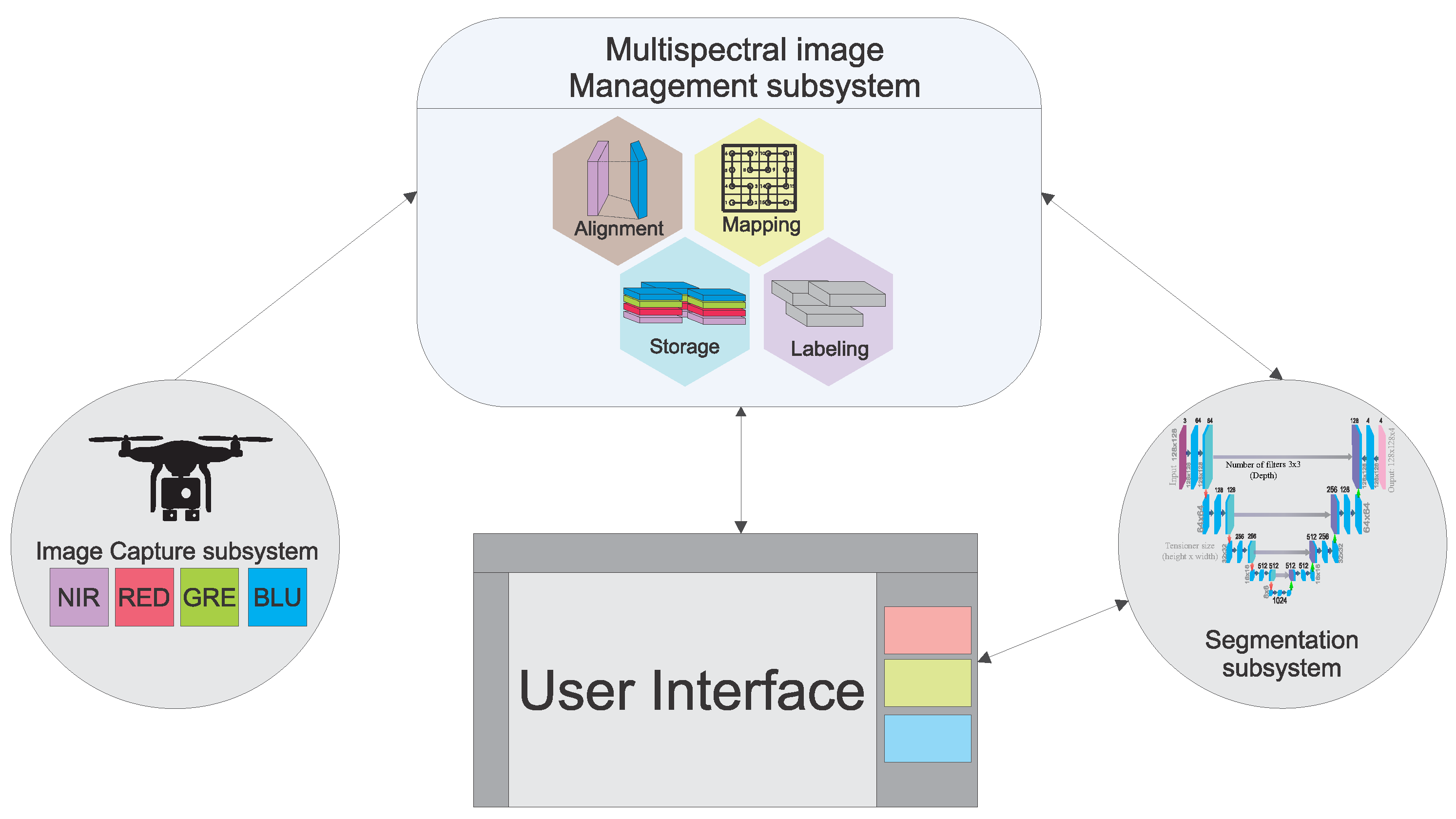
The proposed methodology was applied and validated in a real-world scenario over a 20,000 ${\mathbf{m}}^{\mathbf{2}}$ polyculture farm located in a semi-rural region of Pereira, Colombia. The framework is structured in four main stages, as illustrated in the system architecture in Figure 1. First, the Capture Subsystem collects multispectral data using unmanned aerial vehicles (UAVs) equipped with cameras capable of recording NIR, red, green, and blue channels. Second, this data is processed by the Image Management Subsystem, which integrates modules for data alignment, mapping, labeling, and storage. Third, the processed and labeled data feed the Segmentation Subsystem, which uses deep learning models for automated crop segmentation and NDVI calculation. Finally, the User Interface integrates and visualizes the results, allowing the end-user to interactively manage and analyze the captured data.

3.1. Aerial Multispectral Capture and Storage

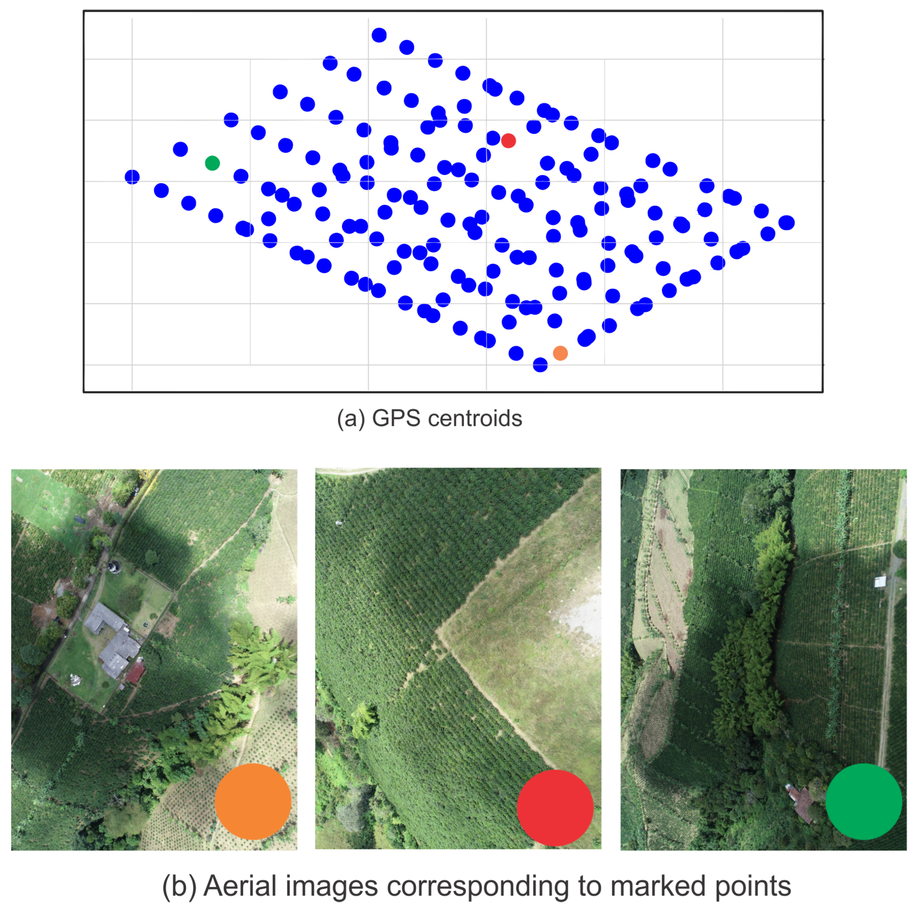
The experimental design focused on the acquisition of multispectral images over a 20,000 m² area in a semi-rural region of Pereira, Colombia. The images were captured using a commercial unmanned aerial vehicle (UAV), the DJI Phantom 4 Pro, manufactured by DJI (Shenzhen, China), and equipped with a Sequoia Sentera^™ multispectral camera (St. Paul, MN, USA). The terrain was divided into a grid of 270 centroids, each corresponding to a 5472 × 3648 pixels image taken from an altitude of 50 m. The distribution of these centroids is illustrated in Figure 2a. The captured images were uploaded to the proposed system, and their corresponding metadata automatically populated the fields of the SQL database. To demonstrate the process, Figure 2b shows the images associated with the colored points marked on the map.

The colors used in both subfigures establish a direct correspondence between Figure 2a and Figure 2b, such that each colored point in the centroid map is associated with the multispectral image marked with the same color. This color-coding scheme enables clear visual identification of the geographic location of each sample image and demonstrates how the proposed system links GPS-based capture points with the images stored in the database.

This dataset was used to validate the performance of the storage and retrieval system. Randomly generated GPS coordinates within the area of interest were used to simulate queries. Additionally, the dataset was expanded by interpolating GPS coordinates within the panoramic image, which allowed for larger-scale testing.

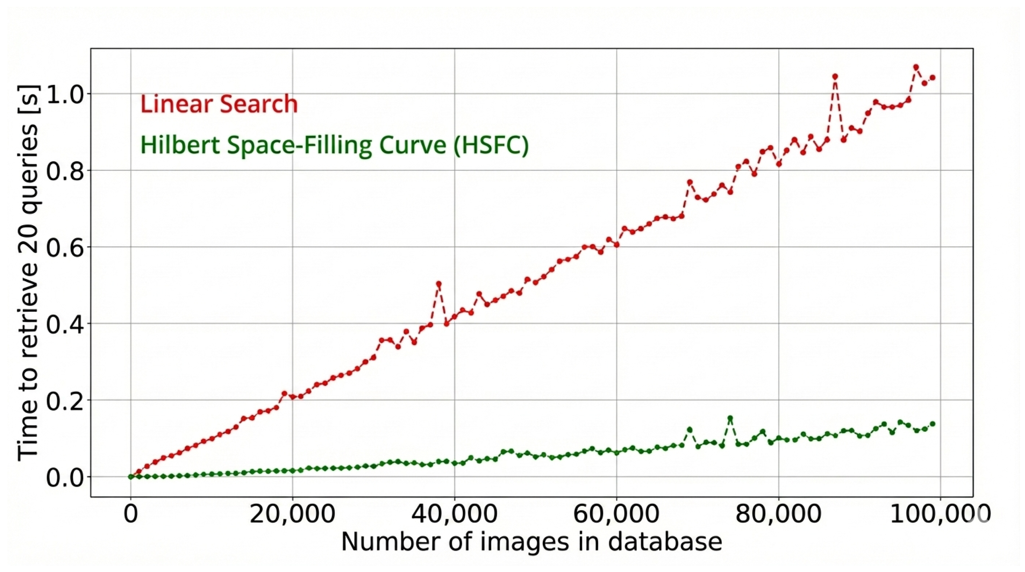
The experiment measured the execution time when querying the database by GPS coordinates, regardless of whether they matched the HSFC centroids. The results were compared to a linear search method that locates the centroid by minimum distance. Figure 3 demonstrates that the HSFC method offers superior performance, especially as the dataset size increases. The X-axis represents the number of GPS coordinates (images) in the database, and the Y-axis shows the average execution time for 20 queries.

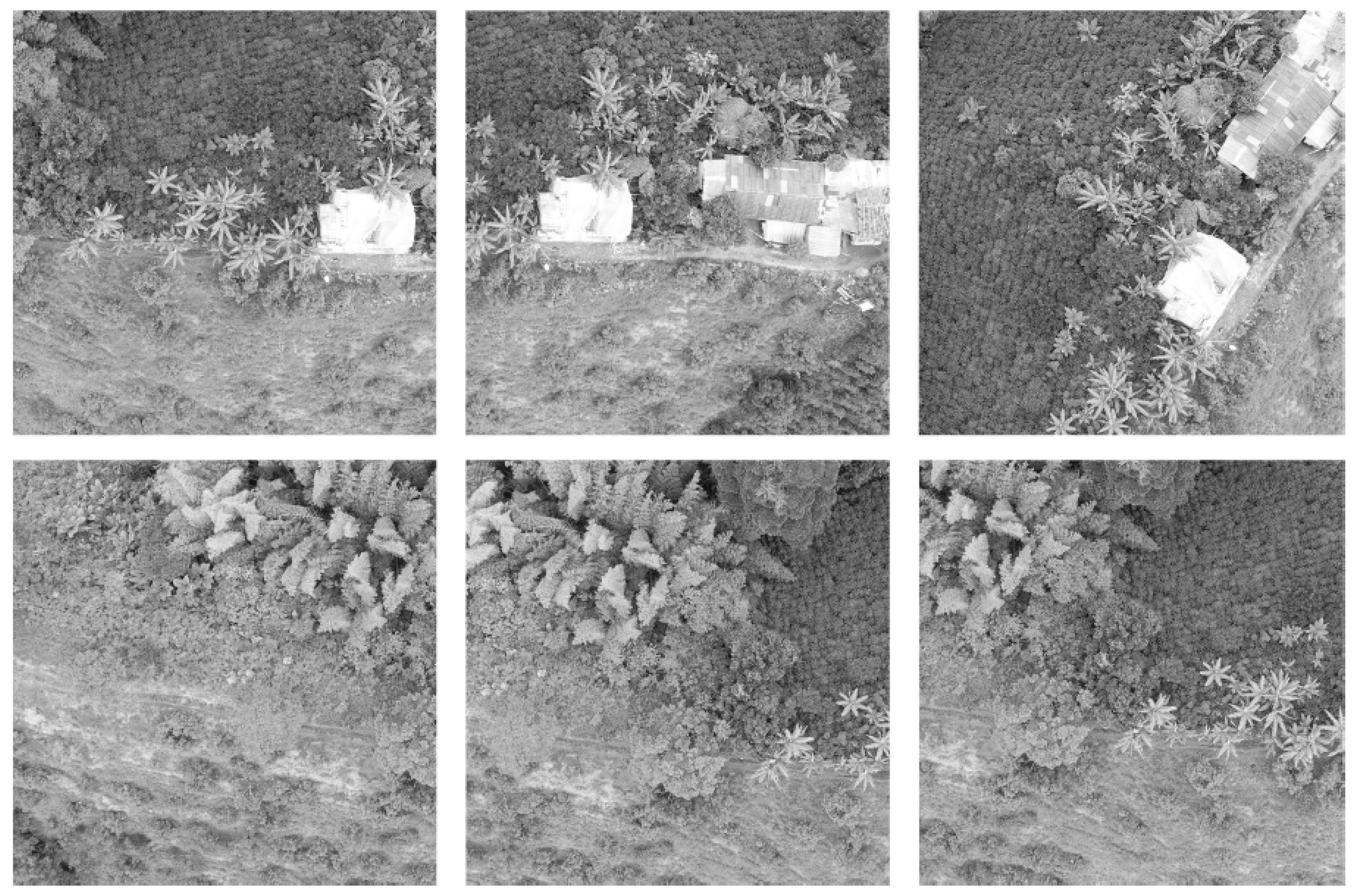
To generate panoramic views, the system retrieves adjacent images by querying the database using the previous and next indices on the HSFC. Figure 4 shows an example of images retrieved with adjacent indices, using the next_index field from the database. These images correspond to the area highlighted in the red box of Figure 5.

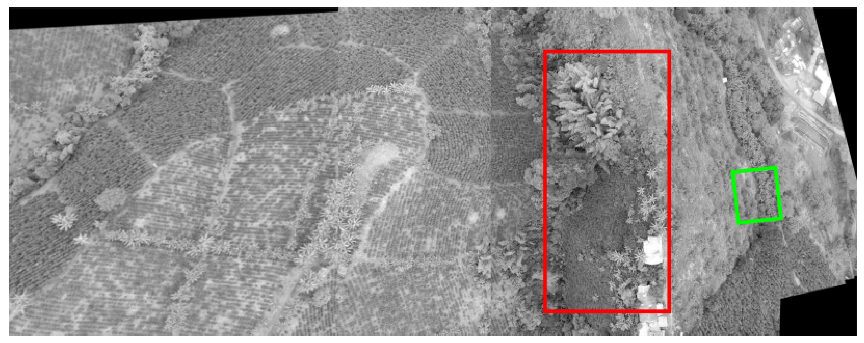
The individual images retrieved are then stitched together to construct a wide-area panorama. Figure 5 presents a panorama composed of 22 images, demonstrating the seamless reconstruction enabled by the HSFC-based retrieval.

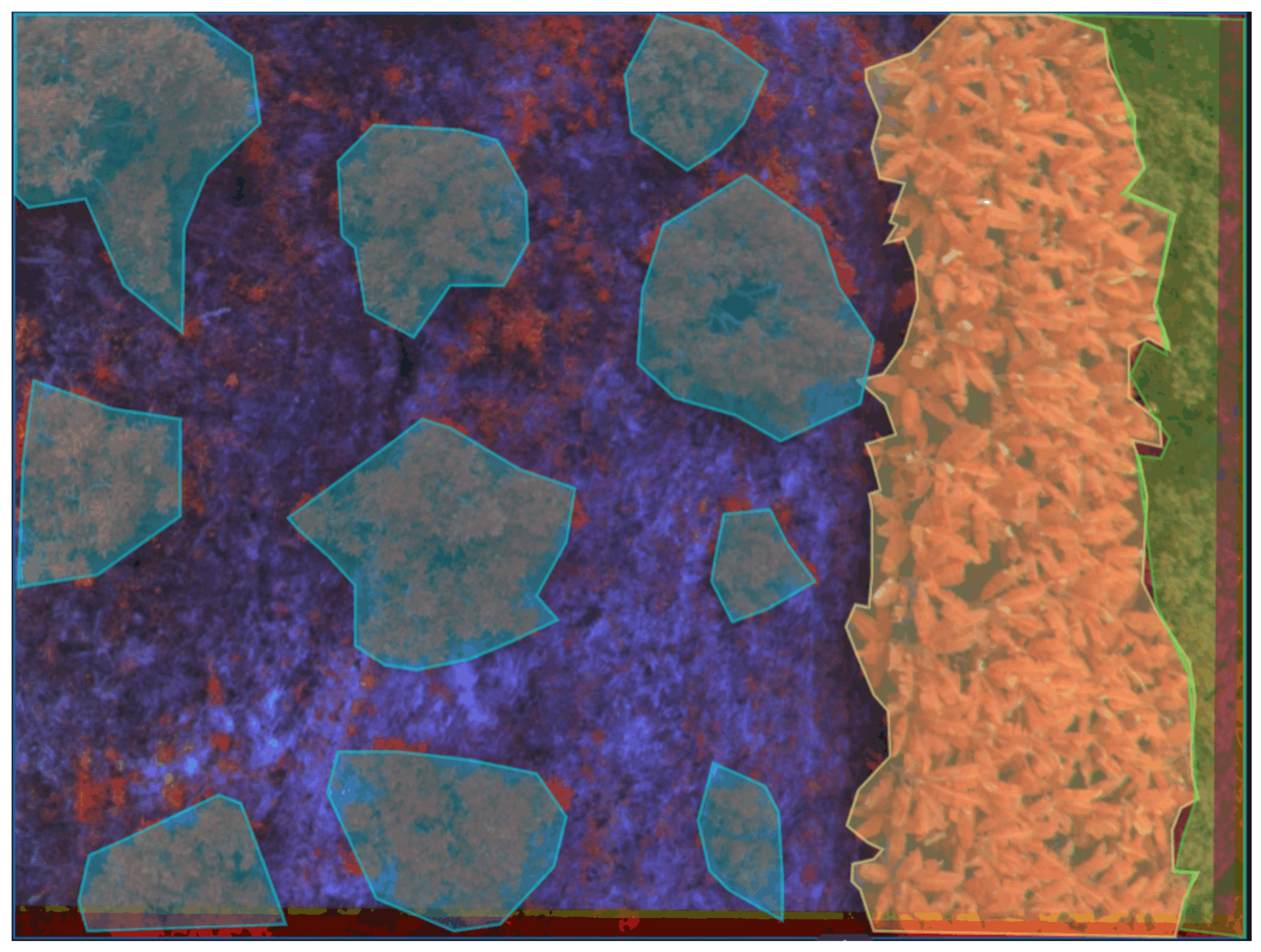
To analyze the raw data utilized for the semantic segmentation task, a specific region of the panoramic view was selected (green box in Figure 5). This region, shown in Figure 6, contains an image composed of the NIR-Red-Green channels along with the generated labels. Each color in the label mask represents a specific class (coffee, plantain, avocado, or soil), which served as the ground truth for training the U-Net model.

The Figure 6 shows the semantic segmentation process by comparing the false-color original images (NIR–Red–Green), the manually annotated labels, and the masks generated by the proposed model. The chromatic differentiation enables a clear identification of the different land covers present in the scene, facilitating the discrimination between coffee, avocado, and plantain crops, as well as soil.

3.2. Data Acquisition System and Image Alignment

The aerial imaging system consists of a fleet of UAVs. For this work, we used the DJI Phantom 4 Pro™ drone, operated using the DJI GO 4 application (version 4.x), which was employed to configure the flight parameters and control image acquisition, and equipped with the Sentera Sequoia™ multispectral camera. The detailed technical specifications of the equipment are provided in

Table 1. Technical Specifications of the UAV and Multispectral Sensor.

DJI Phantom 4 Pro
Manufacturer	DJI (China)
Maximum Flight Time	≈30 min
Maximum Speed	20 m/s (72 km/h)
Nominal Coverage (per flight)	≈65 hectares (at 100 m AGL)
Sentera Sequoia Camera
Sensor Manufacturer	Sentera (USA/France)
Number of Sensors	5 (1 RGB, 4 Monochromatic)
RGB Resolution	5472 × 3648 pixels (20 MP)
Monochromatic Resolution	1280 × 960 pixels (1.2 MP)
Spectral Bands (Central Wavelength)	Green (550 nm), Red (660 nm), Red-Edge (735 nm), NIR (790 nm)
Nominal Ground Sample Distance (GSD)	≈5.3 cm/px (at 50 m AGL)

. The drone was configured to capture images along predefined flight paths with an 80% overlap between consecutive shots. The camera features five lenses to capture RGB, near-infrared (NIR), and red-edge channels. Due to the physical separation of approximately 4 mm between the lenses, a spatial phase shift is introduced, which must be corrected using computer vision techniques. The NIR channel was selected as the reference space, and the remaining channels were aligned through automated homography computation. This alignment was achieved by identifying correspondences between adjacent images and filtering outliers using the RANSAC algorithm. Each drone can capture hundreds or thousands of images, which must be systematically aligned, linked, and stored.

To optimize the coverage of multiple regions and the capture of images at specific centroids, we employ a Linear Temporal Logic (LTL) formula $\phi$. This mathematical formalism allows for the high-level specification of the UAVs’ mission, such as “visit regions $r_1,r_2,\dots ,r_n$ in a specific sequence” or “periodically monitor region A”. The LTL formula is converted into a Büchi automaton, which is a state machine that accepts infinite input sequences satisfying $\phi$. By constructing a product automaton between the UAV’s transition system (representing physical movement capabilities) and the Büchi automaton (representing the task), an optimal path is synthesized. This trajectory minimizes the accumulated cost function (distance or energy) while mathematically guaranteeing that the complex coverage specifications are met.

3.3. Image Storage and Retrieval System

To efficiently manage the storage and retrieval of multispectral images covering large agricultural areas, we implemented a distributed architecture based on the HDFS. This system is designed to handle the massive volume of data generated by UAV fleets, where a single survey can consist of hundreds or thousands of individual snapshots. The HDFS framework stores both the raw multispectral images and their associated metadata, including file paths, GPS coordinates, timestamps, semantic labels, and image descriptors.

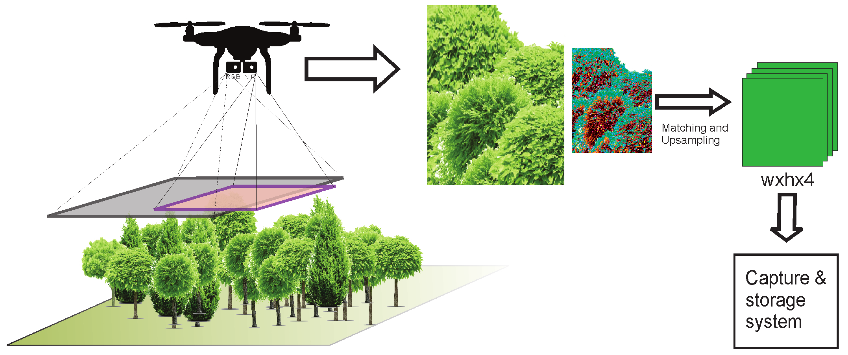
Retrieval and management are facilitated through Apache Hive™ v2.1.1, which provides a SQL-like interface for querying the distributed data. Figure 7 presents a simplified schematic of this workflow, illustrating the path from UAV capture to storage.

To optimize spatial queries, specifically those based on GPS coordinates to identify images within a region of interest, the system employs a Hilbert space-filling curve. This technique transforms multidimensional geospatial coordinates into a linear index, significantly reducing the computational complexity of the search process [30]. Finally, a custom interface developed Python 3.8 connects to this infrastructure, allowing users to execute metadata-based queries, download specific multichannel images, and manage the stored records, providing the necessary flexibility and robustness for big data applications.

To formalize the retrieval process described above, Algorithm 1 details the computational steps for querying images based on geospatial proximity using the HSFC index. This approach minimizes the search space before applying precise Euclidean distance filtering.

Algorithm 1 HSFC-Based Image Retrieval Strategy

Require:  Target GPS coordinates $(la{t}_q,lo{n}_q)$, Search Radius R, Hilbert Order N Ensure:  List of retrieved images $L_{final}$   1: Step 1: Coordinate Transformation   2: $P_{xy}\leftarrow \mathrm{GeoToCartesian}(la{t}_q,lo{n}_q)$   3: $H_{target}\leftarrow \mathrm{HilbertMapping}(P_{xy},N)$ {Calculate linear index}   4: Step 2: Define Search Range in Hilbert Space   5: $\Delta H\leftarrow \mathrm{EstimateHilbertRange}(R,N)$   6: $H_{min}\leftarrow H_{target}-\Delta H$   7: $H_{max}\leftarrow H_{target}+\Delta H$   8: Step 3: Database Query (SQL/Hive)   9: $Query\leftarrow “\mathrm{SELECT} * \mathrm{FROM} \mathrm{images} \mathrm{WHERE} \mathrm{h}\_\mathrm{index} \mathrm{BETWEEN} H_{min} \mathrm{AND} H_{max}^{″}$ 10: $Candidates\leftarrow \mathrm{ExecuteQuery}\left(Query\right)$ {Initial filtering $O(logn)$} 11: Step 4: Precise Filtering (Spatial Continuity) 12: for all $img\in Candidates$ do 13:  $d\leftarrow \mathrm{EuclideanDistance}(img.gps,(la{t}_q,lo{n}_q))$ 14:  if $d\le R$ then 15:   $L_{final}.append\left(img\right)$ 16:  end if 17: end for 18: return  $L_{final}$

3.4. Content-Based Image Retrieval

We propose a Content-Based Image Retrieval (CBIR) system to query the database using criteria such as GPS coordinates, crop species, or water status. The retrieved images are stitched together to generate a panoramic view of the area, while the associated labels are processed to create a segmentation mask covering the entire region. These labels can be generated manually by an operator through the system or automatically by the deep semantic segmentation neural network, which is detailed in Section 3.6.

The images and labels have over 50% overlap, ensuring accurate stitching. The geometric registration of adjacent images is performed by applying the homography matrices previously computed during the initial alignment phase, ensuring a seamless geometric transformation for panoramic reconstruction. Since multiple labels may coexist for the same pixel, the stitching algorithm calculates a weighted average to resolve discrepancies and merge the overlapping regions seamlessly. This weighting is based on a distance function that assigns a higher confidence (weight) to the pixel closer to the center of its original image, effectively creating a smooth blend (feathering) and minimizing visible seams in the final output.

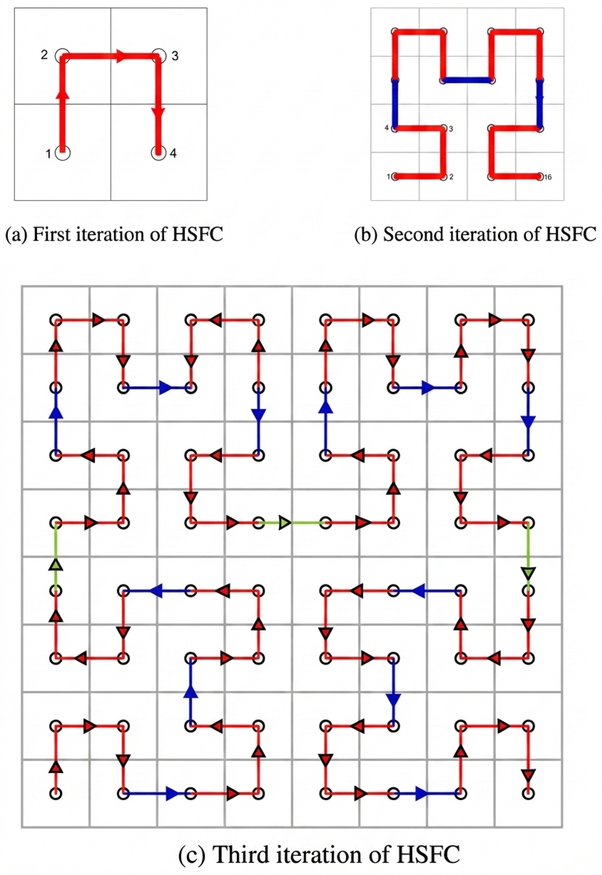
To reduce the complexity of retrieval by GPS coordinates, we use a HSFC to map points from ${\mathbb{R}}^2$ to $\mathbb{R}$. Assuming a square space divided into four quadrants, the curve traverses the centroids of these subdivisions. Figure 8 illustrates the first three iterations of the HSFC. Recursively, each subdivision can be divided into four smaller sections, which are rotated 90 degrees to connect adjacent spaces. The order of the HSFC is defined by the number of iterations, as shown in the figure.

It is important to note that while HSFC efficiently clusters spatially local points, it contains inherent discontinuities where sequential indices may be geographically distant (e.g., the jump between quadrants). To address this limitation for panoramic generation, we employ a hybrid retrieval strategy. The HSFC is primarily used to rapidly narrow down the search space to a candidate block with $O(logn)$ complexity. Once retrieved, a secondary spatial filter based on Euclidean distance (using GPS coordinates) is applied to the candidate images to strictly select the immediate geographical neighbors required for accurate stitching, ensuring spatial continuity regardless of HSFC index jumps.

Mapping points from a plane to an n-order HSFC requires an affine transformation, dividing the space into square intervals of $2^n$. The HSFC sequence can be represented in matrix form, as shown in Equations (1)–(4), where $(x_1,x_2)$ are the coordinates of a point in the unit square and $Q_n$ is the corresponding subsquare.

$$Q_0\left(\begin{array}{c}{x}_1\\ x_2\end{array}\right)={\displaystyle \frac{1}{2}}\left(\begin{array}{cc}0& 1\\ 1& 0\end{array}\right)\left(\begin{array}{c}{x}_1\\ x_2\end{array}\right)+{\displaystyle \frac{1}{2}}\left(\begin{array}{c}0\\ 0\end{array}\right)$$

(1)

$$Q_1\left(\begin{array}{c}{x}_1\\ x_2\end{array}\right)={\displaystyle \frac{1}{2}}\left(\begin{array}{cc}1& 0\\ 0& 1\end{array}\right)\left(\begin{array}{c}{x}_1\\ x_2\end{array}\right)+{\displaystyle \frac{1}{2}}\left(\begin{array}{c}0\\ 1\end{array}\right)$$

(2)

$$Q_2\left(\begin{array}{c}{x}_1\\ x_2\end{array}\right)={\displaystyle \frac{1}{2}}\left(\begin{array}{cc}1& 0\\ 0& 1\end{array}\right)\left(\begin{array}{c}{x}_1\\ x_2\end{array}\right)+{\displaystyle \frac{1}{2}}\left(\begin{array}{c}1\\ 1\end{array}\right)$$

(3)

$$Q_3\left(\begin{array}{c}{x}_1\\ x_2\end{array}\right)={\displaystyle \frac{1}{2}}\left(\begin{array}{cc}0& -1\\ -1& 0\end{array}\right)\left(\begin{array}{c}{x}_1\\ x_2\end{array}\right)+{\displaystyle \frac{1}{2}}\left(\begin{array}{c}2\\ 1\end{array}\right)$$

(4)

3.5. Labeled Dataset Creation

Training deep learning models requires a large, labeled dataset with local crop species, such as coffee, plantain, and avocado. The first step after acquiring multispectral images is the spatial alignment of the five color layers. This is achieved by computing keypoints with scale- and rotation-invariant algorithms like Oriented FAST and Rotated BRIEF (ORB), Scale-Invariant Feature Transform (SIFT), or Speeded-Up Robust Features (SURF). With at least four corresponding keypoints, homographies are calculated to project the images into a common alignment space.

The second step is the calculation of the NDVI mask from the aligned images, defined by Equation (5):

$$NDVI={\displaystyle \frac{NIR-R}{NIR+R}},$$

(5)

where $NIR$ represents the near-infrared channel (central wavelength of 790 nm) and R represents the red channel (central wavelength of 660 nm). Subsequently, the resulting images are uploaded via FTP to a data warehouse.

The third step is manual labeling, performed with a tool based on LabelMe v4.5.13. This software allows drawing polygons for semantic segmentation and storing them in XML or JSON format. These labels are then converted to a single-channel PNG image. Four labels were defined: (1) soil, (2) coffee crop, (3) plantain crop, and (4) avocado crop. Once verified, the labels are uploaded to the management system, updating the registry to distinguish between labeled and unlabeled images. In the PNG layers, pixel values (0 to 3) represent each semantic label.

3.6. Semantic Segmentation Model for Crop Species Detection

Crop management with aerial images generates large volumes of data. Authors such as [31,32] have employed deep learning architectures like U-Net to solve precision agriculture problems, with promising results in land cover classification and corn water status. Additionally, ref. [29] presented variations of U-Net that improve upon the original architecture’s performance at the cost of higher memory usage.

The U-Net architecture consists of two main paths: a contraction path (encoder) and an expansion path (decoder). The encoder extracts a dense feature map by progressively reducing resolution through convolutional and max-pooling layers. The decoder takes this low-resolution feature map and gradually reconstructs it to the original size through upsampling and convolution operations. To mitigate the vanishing gradient problem [33], U-Net incorporates skip connections that link encoder layers with their counterparts in the decoder, reusing features and accelerating training.

We selected U-Net for automatic labeling for two key advantages. First, it requires a relatively small dataset to achieve good results, as demonstrated in [33,34] where they trained with only 35 images using data augmentation. Second, its low memory consumption allows for deploying the inference model on embedded systems like Nvidia Jetson Nano™ for real-time labeling.

The U-Net model is trained using the Categorical Cross-Entropy loss function, which is the standard for multi-class segmentation tasks. The mathematical formulation of the loss function and the final segmentation mask generation via the Softmax activation function are detailed in Section 4.1, where the optimization strategies are discussed.

To evaluate performance, the authors in [35] use the intersection over union (IoU) metric, or Jaccard index, which measures the degree of overlap between the predicted and ground-truth labels, as defined in Equation (6):

$$IoU={\displaystyle \frac{|A\cap B|}{|A\cup B|}},$$

(6)

where A is the set of predicted pixels and B is the set of ground-truth pixels. The numerator represents the intersection and the denominator, the union of both sets.

4. Experiments

4.1. Crop Semantic Segmentation

For model training, manual labeling was performed by marking the different plant types with the developed tool. In this work, three common crops from the Pereira region were labeled: plantain, avocado, and coffee, as seen in Figure 6 (green box in Figure 5). The dataset, comprising 270 multispectral images, was split into 70% for training and 30% for validation. Three spectral bands (NIR, Red, and Green) were used, and the images were resized to 128 × 128 pixels to accommodate GPU memory limitations. The selection of these three specific bands was made to prioritize computational efficiency and direct relevance to the final objective. The NIR and Red bands are essential for calculating the NDVI, which is the primary health indicator used in the methodology. The Green band was included as it provides complementary information for differentiating the chlorophyll content of the distinct crop species. Crucially, limiting the input to three channels ($128\times 128\times 3$) allowed the model to be trained and deployed on a system with only 8 GB of VRAM (as detailed below), making the entire framework compatible with low-cost embedded devices like the Nvidia Jetson Nano.

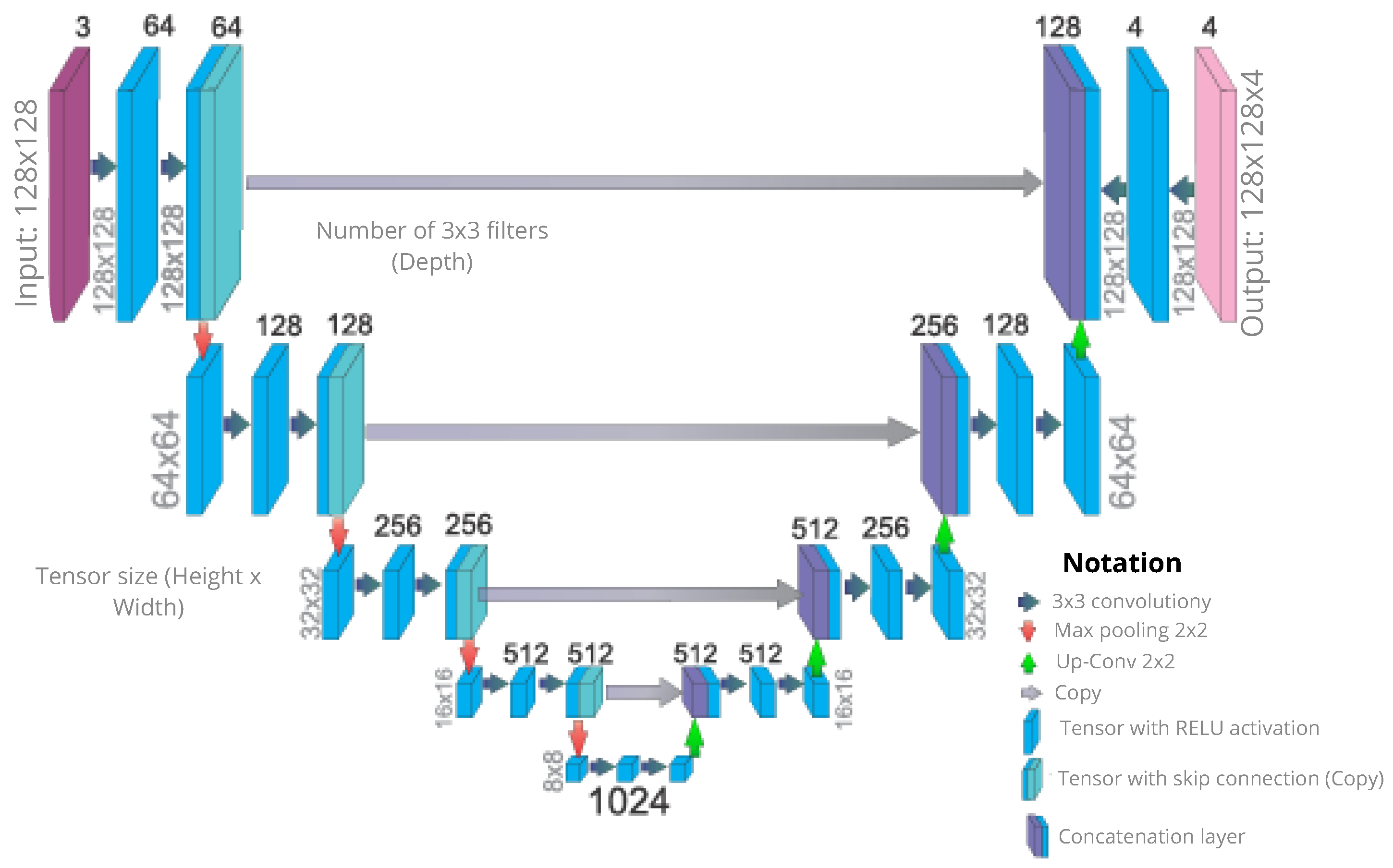
The U-Net model processes 128 × 128 × 3 input tensors and generates 128 × 128 × 4 outputs, corresponding to the four target classes (avocado, plantain, coffee, and soil). The model employs the Categorical Cross-Entropy loss function, which is the standard formulation for multi-class segmentation problems. Unlike binary formulations, this function penalizes the divergence between the predicted probability distribution and the ground truth distribution across all K classes:

$$J=-\sum _{c=1}^K{y}_{o,c}log\left(p_{o,c}\right),$$

(7)

where K is the number of classes (4 in this study), $y_{o,c}$ is the binary indicator (0 or 1) if class label c is the correct classification for observation o, and $p_{o,c}$ is the predicted probability. A softmax function is applied to the output to obtain the final segmentation mask:

$$\sigma {\left(Z\right)}_j={\displaystyle \frac{e^{Z_j}}{{\sum }_{k=1}^K{e}^{Z_k}}},$$

(8)

where Z represents the input vector to the softmax function and $\sigma {\left(Z\right)}_j$ is the probability of the j-th class.

The U-Net model employed for semantic segmentation follows an encoder–decoder architecture designed to extract hierarchical features and reconstruct segmentation maps with high spatial accuracy. This architecture, illustrated in Figure 9, combines contraction and expansion paths connected through skip connections, allowing the preservation of contextual information and relevant spatial details during the reconstruction of the segmented masks.

Regarding the dataset size, we acknowledge that 270 multispectral images represents a limited sample size. However, the robustness of the segmentation model is ensured through three key strategies. First, the high dimensional density of multispectral data (4 channels per capture) provides significantly richer feature sets compared to standard RGB imagery. Second, to overcome the scarcity of labeled data, we employed a Transfer Learning approach. The U-Net encoder was initialized with weights pre-trained on ImageNet, allowing the model to leverage learned low-level feature extractors (edges, textures) and focusing the training process solely on fine-tuning the weights for the specific spectral signatures of the crops. Finally, a rigorous data augmentation pipeline was applied, performing 6 distinct transformations per image (including random rotations $\pm {15}^{\circ }$, flips, zoom, and brightness shifts). This effectively expanded the training dataset to over 1600 training samples, providing sufficient variability to mitigate overfitting and achieve generalizable results.

The experiments were conducted using a rigorous configuration to ensure reproducibility. The specific hyperparameters utilized were: a batch size of 4, a categorical cross-entropy loss function, and a fixed seed for initialization. Two optimizers were evaluated:

1.

Adam: An adaptive optimizer with a standard learning rate of $5\times {10}^{-3}$, ${\beta }_1=0.9$ and ${\beta }_2=0.999$.

2.

Radam [34]: A variant that implements individual learning rates per parameter with an automated warm-up phase.

Experimental results showed that ADAM suffered from convergence issues at this learning rate, likely getting trapped in poor local minima early in the training process (underfitting), which explains its significantly lower performance and slower convergence time (25 h). In contrast, Rectified Adam (RAdam) employs a dynamic rectifier to adjust the adaptive momentum. This allowed the model to stabilize training quickly despite the relatively high learning rate and the small batch size. The final evaluation on the independent Test Set (30% of data) yielded a Mean Intersection over Union (MIoU) of 68.4% for the RAdam model, confirming its superiority for this specific dataset.

A quantitative comparison of the optimization strategies evaluated in this study is presented in

Table 2. Comparison of optimizer performance on the Test Set. Note: ‘Convergence Time’ refers to the time taken to reach the best validation score before early stopping.

Optimizer	Learning Rate	Batch Size	Test Set MIoU [%]	Convergence Time [Hours]
ADAM	$5\times {10}^{-3}$	4	40.1	25
RADAM	$5\times {10}^{-3}$	4	68.4	3.5

. The table summarizes the learning rate, batch size, convergence time, and segmentation performance on the independent Test Set for both optimizers.

Computational Cost and Efficiency Analysis

To address the disparity in total training time (25 h vs. 3.5 h) and validate the absence of hidden variables, we performed a detailed analysis of computational costs. The experiments were executed on a workstation equipped with an Nvidia GeForce GTX 1080 (8 GB VRAM).

The computational cost per epoch was consistent across both optimizers, averaging ≈3.7 min per epoch given the dataset size and augmentation overhead. The significant difference in total training time is attributed solely to the convergence rate:

• Adam: Failed to minimize the loss effectively, triggering the maximum training duration (stopped at ≈400 epochs) without achieving satisfactory validation scores.
• RAdam: The automated learning rate warm-up allowed the model to reach the early stopping criteria rapidly, converging in approximately 56 epochs.

To further validate the multi-class segmentation performance,

Table 3. Detailed Classification Report and IoU per Semantic Class (Test Set).

Class	Precision	Recall	F1-Score	IoU [%]
Coffee (Class 0)	0.94	0.91	0.93	86.9
Plantain (Class 1)	0.83	0.82	0.82	69.5
Avocado (Class 2)	0.79	0.89	0.83	70.9
Soil (Class 3)	0.89	0.90	0.90	81.8
Macro Average	0.86	0.88	0.87	77.3

details the Precision, Recall, F1-Score, and Intersection over Union (IoU) for each of the four semantic classes. These metrics are derived from the confusion matrix obtained on the test set.

The confusion matrix confirms that the model successfully discriminates between the vegetative classes, with particularly high performance in Coffee crops (F1-Score 0.93), demonstrating the effectiveness of the Categorical Cross-Entropy loss function utilized.

4.2. Discussion on Model Selection: Accuracy vs. Efficiency

While state-of-the-art architectures such as DeepLabV3+, SegFormer, or the Segment Anything Model (SAM) offer impressive segmentation capabilities, our selection of the U-Net architecture is grounded in the specific constraints of precision agriculture using embedded UAV systems.

First, regarding computational efficiency, this study targets deployment on resource-constrained edge devices like the Nvidia Jetson Nano (4 GB/8 GB RAM). Modern Transformer-based models (e.g., SegFormer) or foundational models (e.g., SAM) entail a high computational overhead (FLOPS) and memory footprint that make them unsuitable for real-time, on-board inference without heavy quantization or cloud offloading, which is often unavailable in rural areas. U-Net offers an optimal trade-off, providing sufficient segmentation accuracy (68.4% MIoU) with a lightweight CNN structure capable of efficient inference on embedded hardware.

Second, regarding data availability, Transformer-based models typically lack the inductive biases of CNNs and require massive datasets to converge without overfitting. Given our limited dataset (1620 augmented images), the CNN-based U-Net is more advantageous for generalization via Transfer Learning, as demonstrated by its established success in medical imaging contexts with similar data scarcity.

5. Discussion of Resuts

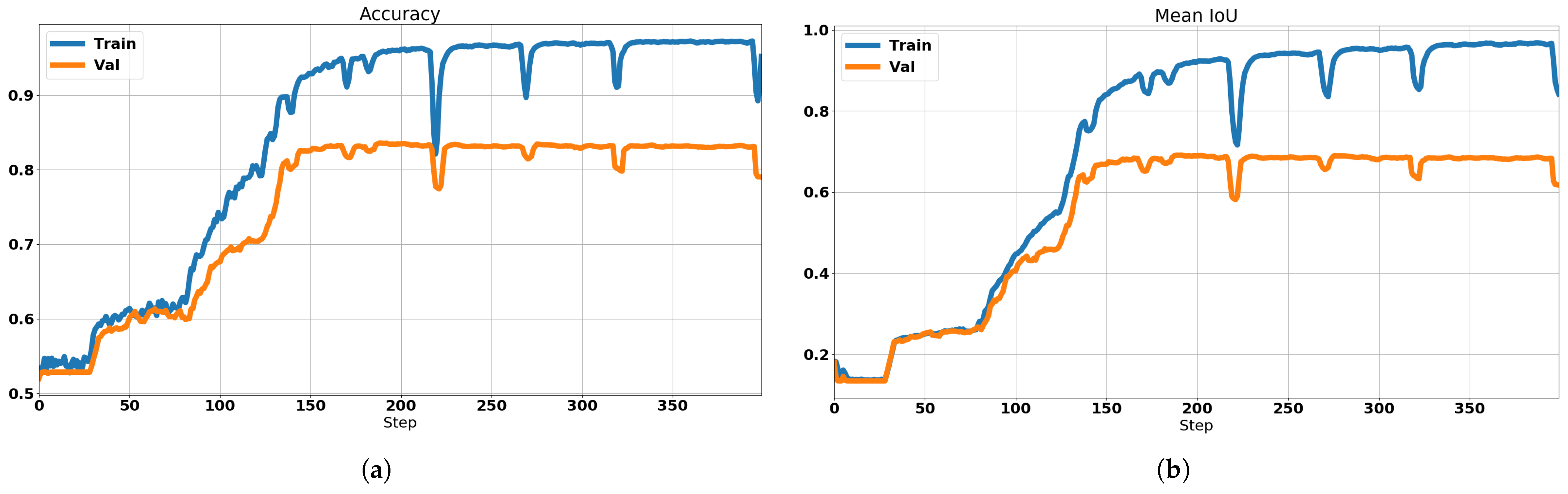
The evaluation of the semantic segmentation model yielded results that demonstrate the viability of the proposed approach for crop species characterization in polyculture environments. Figure 10a shows the model’s accuracy during training, where it achieved an average accuracy of 82.3% on the test set, while the MIoU metric reached 68.4% during inference, as illustrated in Figure 10b.

The MIoU of 68.4% indicates that the model effectively distinguishes between different crop species (coffee, plantain, and avocado) as well as soil, although there is substantial room for improvement. According to [34], MIoU values above 65% are considered acceptable for real-time applications, particularly when computational efficiency is prioritized. The encoder-decoder architecture employed in this work follows the principles established by [36], who demonstrated that these networks can be effectively trained with limited datasets through aggressive data augmentation strategies. In their seminal work on biomedical image segmentation, ref. [36] showed that U-Net architectures can achieve accurate segmentation with as few as 30 training images when combined with elastic deformations and other augmentation techniques.

The training curve in Figure 10a shows stable convergence without significant overfitting. This behavior aligns with the findings of [37], who pioneered fully convolutional networks for semantic segmentation and achieved 62.2% mean IU on PASCAL VOC 2012. Their work demonstrated that end-to-end pixel-to-pixel training enables CNNs to learn hierarchical feature representations suitable for dense prediction tasks. Similarly, ref. [34] reported that encoder-decoder architectures maintain good performance while being significantly more memory-efficient than alternative approaches such as FCN or DeconvNet.

The achieved accuracy of 82.3% is consistent with performance reported in related agricultural applications. For example, ref. [21] developed a semantic segmentation framework for weed mapping using aerial multispectral images and deep neural networks, achieving 86.3% accuracy in crop detection and 78.2% in weed identification over areas exceeding 16,500 m². Their work emphasized that semantic segmentation plays a crucial role in crop monitoring and agricultural scene understanding, which directly relates to polyculture characterization.

However, current performance suggests that expanding the training dataset could yield significant improvements. Ref. [37] demonstrated that their FCN-8s architecture achieved substantial gains when trained on larger datasets, improving from 62.2% to 67.2% mean IU by incorporating additional training data. This observation is particularly relevant to our work, as it suggests that targeted data collection focused on underrepresented crop configurations could significantly improve model generalization.

Furthermore, the encoder-decoder architecture used in this study could benefit from transfer learning strategies. Ref. [34] showed that initializing the encoder with weights pre-trained on large-scale datasets such as ImageNet can improve segmentation performance by approximately 8 to 12 percentage points compared to random initialization. This approach could be explored in future iterations to enhance our model’s feature extraction capabilities without necessarily requiring massive amounts of labeled crop data.

The results also compare favorably with recent applications of semantic segmentation in precision agriculture. Ref. [29] proposed modifications to the U-Net architecture to improve crop segmentation in mixed-cropping scenarios, demonstrating the need to adapt neural networks to the particularities of complex agricultural systems. A recent study by [25] developed a multimodal model that combines multispectral images with meteorological data to predict rice yield, achieving an RMSE of only 0.859 t/ha, demonstrating the potential of integrating multiple data sources in precision agriculture applications.

These achieved results demonstrate that the proposed methodology is feasible for real-time characterization of crop species in polyculture environments. The model has successfully learned meaningful spatial representations of the different species (coffee, plantain, avocado) and soil, as evidenced by stable training convergence and acceptable MIoU performance. Future work should focus on expanding the training dataset through image capture at different phenological stages and lighting conditions, as well as exploring transfer learning strategies to push performance toward the 80–85% MIoU range, which would represent state-of-the-art performance for this specific precision agriculture application.

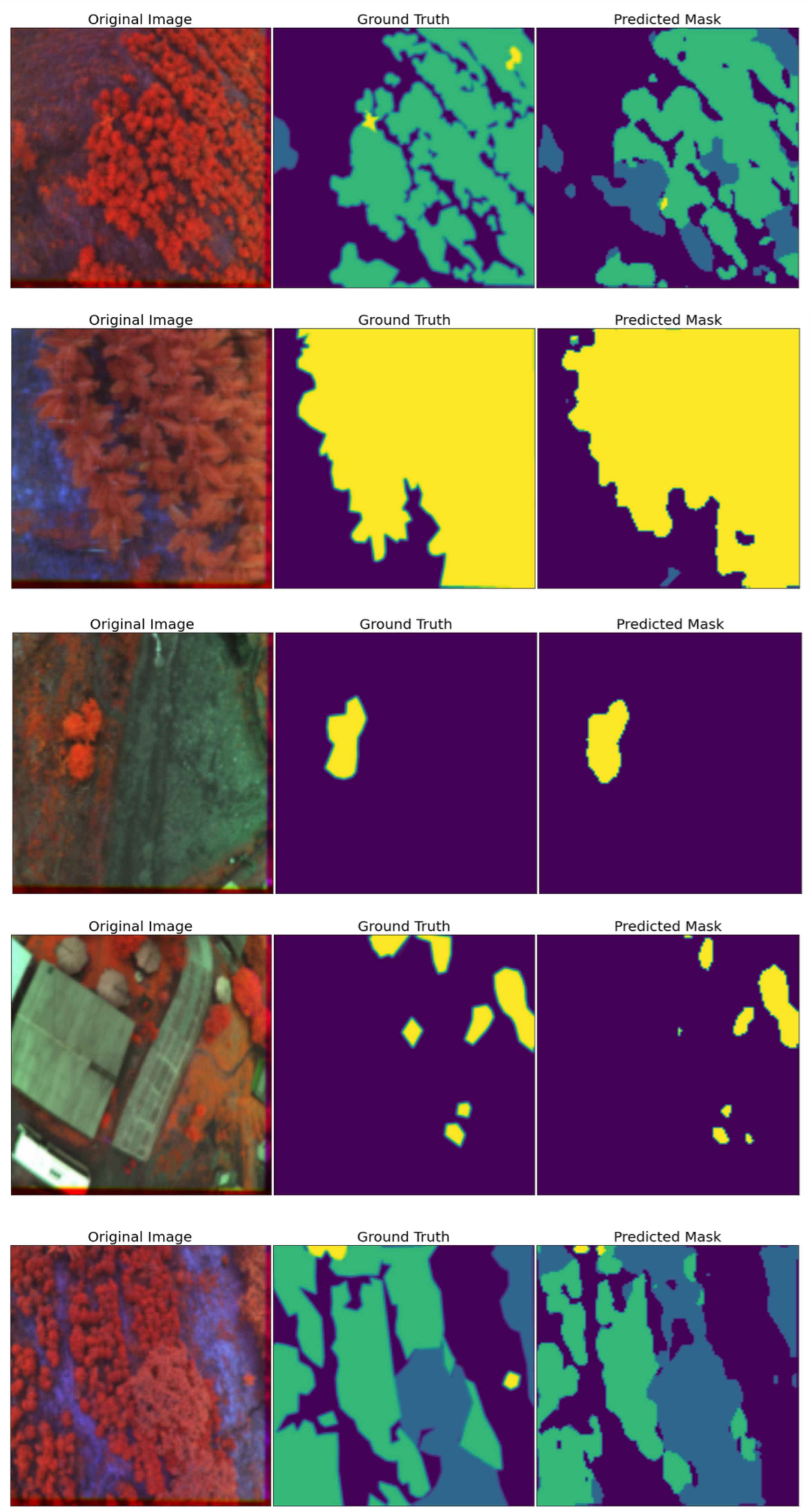
To facilitate the visual interpretation of the semantic segmentation results,

Table 4. Color Key for Semantic Segmentation Maps (Figure 11).

Class	Pixel Value	Color in Ground Truth (Center Column)
Coffee	0	Green
Plantain	1	Yellow
Avocado	2	Dark Green
Soil	3	Dark Purple

presents the correspondence between each land cover type and its chromatic representation in the segmentation maps shown in Figure 11.

Figure 11 presents visual examples of the results from the U-Net semantic segmentation algorithm. The left column shows the original crop image (a NIR-Red-Green composite). The center column displays the manually created and validated ground truth labels. The right column presents the predictions generated by the model. This comparison allows for a qualitative assessment of the model’s ability to accurately segment the different crops and the soil, highlighting its successes and areas for improvement, especially in delineating the boundaries between classes.

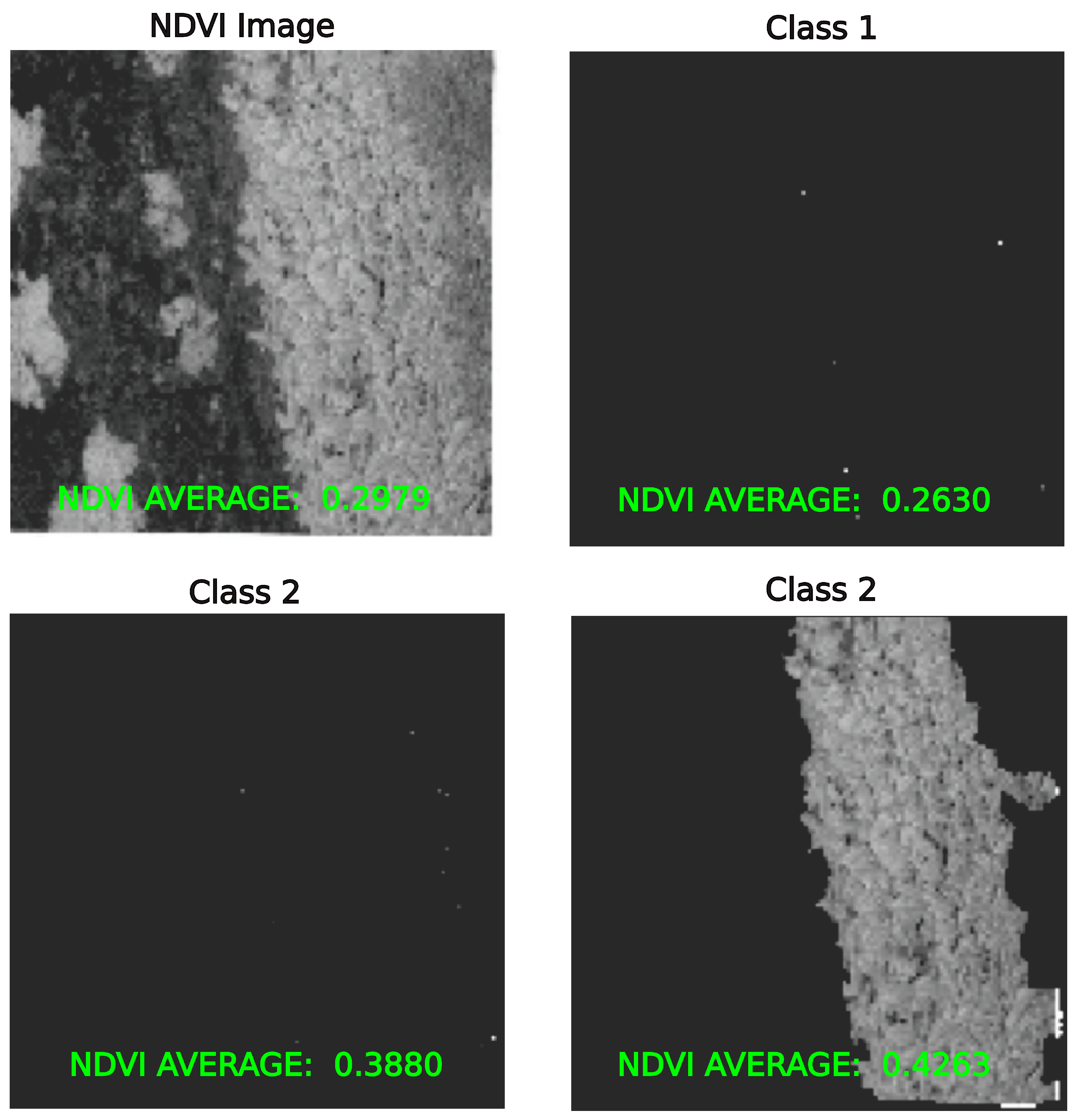
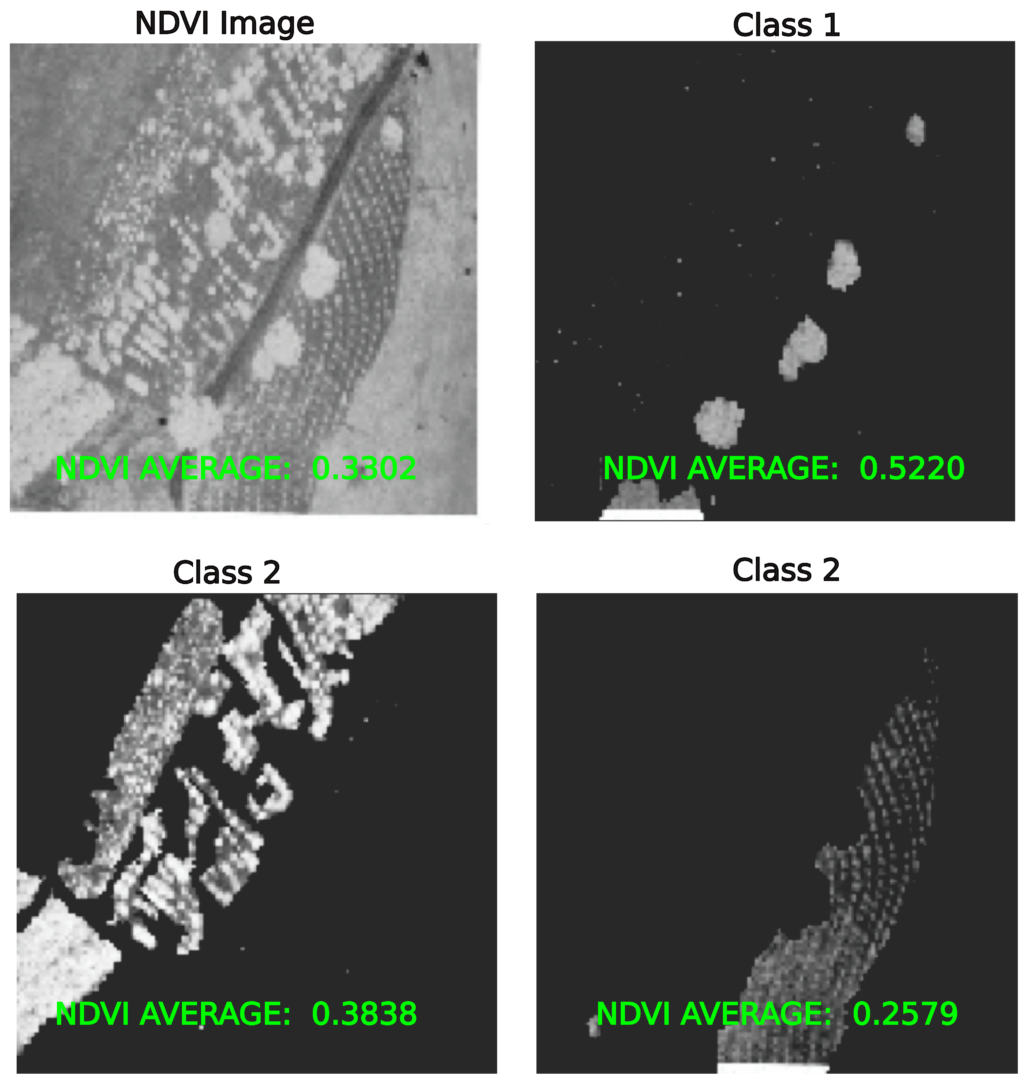
The NDVI calculation was refined by using the semantic segmentation masks, which allowed the analysis to focus on specific crop species. Figure 12 exemplifies this process, highlighting areas with high NDVI values (healthy vegetation) and low values (stressed vegetation or bare soil).

Figure 13 takes this a step further, comparing the NDVI distributions between coffee and plantain crops. This visualization clearly illustrates the differences in vegetation health and vigor between the two species, underscoring the utility of species-specific NDVI calculations for precision monitoring.

5.1. Limitations of the Study

Despite the satisfactory performance reported, this study presents specific limitations that must be addressed in future research to ensure broad scalability. First, regarding computational scalability, while the HDFS architecture allows for massive storage, the synchronization between UAVs and the cloud is constrained by the limited network bandwidth available in rural agricultural areas. This creates a bottleneck when uploading terabytes of multispectral data, suggesting that a more robust edge-computing compression strategy is needed.

Second, regarding model generalization, the U-Net was trained exclusively with data from a specific region in Pereira, Colombia. Consequently, the model may experience performance degradation when applied to crops with different phenological stages or under different lighting conditions (e.g., severe shadows or cloud cover), known as the domain shift problem. Finally, while the HSFC optimizes retrieval, the stitching process still heavily relies on accurate GPS data; in scenarios with GPS signal degradation, the reconstruction of panoramic views could be compromised. Addressing these challenges through on-board pre-processing and domain adaptation techniques remains a priority for future work.

5.2. Accuracy vs. Efficiency

While state-of-the-art architectures such as DeepLabV3+, SegFormer, or the Segment Anything Model (SAM) demonstrate superior segmentation performance on benchmark datasets, our selection of the U-Net architecture is rigorously justified by the specific computational, operational, and data constraints of embedded precision agriculture systems. The experimental evaluation presented in Section 4.2 demonstrates that U-Net achieves an accuracy of 82.3% and a Mean Intersection over Union (MIoU) of 68.4% on our polyculture dataset of 270 multispectral images (1620 after augmentation including rotations, flips, zoom, and brightness shifts). This performance was achieved using a dataset partitioned into 70% for training and 30% for validation, with images resized to 128 × 128 pixels to accommodate the 8 GB VRAM limitations of our target deployment hardware.

The selection of three spectral bands (NIR, Red, and Green) was made to prioritize computational efficiency while maintaining the capability to calculate NDVI, which is the primary health indicator for this application. The encoder was initialized with ImageNet pre-trained weights, enabling effective transfer learning despite the limited dataset size—a critical advantage compared to Transformer-based models that typically require datasets exceeding 100,000 images to converge without overfitting.

The computational efficiency of U-Net is further evidenced by our training results using the Rectified Adam (RAdam) optimizer with a learning rate of 5 × 10⁻³ and batch size of 4. As detailed in Table 2, RAdam achieved convergence in only 3.5 h with a test set MIoU of 68.4%, compared to the standard ADAM optimizer which required 25 h yet achieved only 40.1% MIoU. This 7× reduction in convergence time demonstrates U-Net’s training efficiency on resource-constrained systems. The detailed classification report in Table 3 shows strong per-class performance with F1-scores of 0.93 for Coffee, 0.82 for Plantain, 0.83 for Avocado, and 0.90 for Soil, with individual IoU values ranging from 69.5% to 86.9%.

While more complex Transformer-based architectures might achieve marginally higher MIoU values, this improvement would come at the cost of significantly increased inference time, memory consumption, and power requirements that are operationally prohibitive for embedded UAV systems in rural agricultural settings where network connectivity is limited and real-time processing is essential. The stable training convergence shown in Figure 10a without significant overfitting, combined with the deployment feasibility on low-cost embedded devices like the Nvidia Jetson Nano, positions U-Net as the optimal architectural choice for this precision agriculture application, balancing sufficient segmentation accuracy with operational viability and energy efficiency [27,38,39,40,41].

6. Conclusions

In this paper, we presented a comprehensive methodology for automated crop health monitoring in large areas using multi-spectral images and deep convolutional neural networks, validated in a polyculture farm in Pereira, Colombia. Our method was divided into four integrated subsystems:

First, a capture and management system was designed to efficiently acquire image data using UAVs. Second, we proposed a system for multi-spectral image storage and retrieval. The implementation of the Hilbert Space-Filling Curve successfully reduced the computational complexity of image retrieval based on GPS coordinates from $O\left(n^2\right)$ to $O(logn)$, demonstrating an efficiency critical for big data management.

Third, we proposed a labeling scheme to store both human labels and machine-generated labels, facilitating rapid dataset expansion. Finally, we developed a convolutional neural network framework based on a U-Net model for automatic pixel labeling and discriminating crop species.

The model’s training demonstrated the crucial impact of the optimizer selection: the Rectified Adam (RAdam) algorithm achieved convergence in only 3.5 h, confirming its superiority over the standard ADAM optimizer (25 h). The final evaluation of the semantic segmentation model yielded a robust performance with a Mean Intersection over Union (MIoU) of 68.4%. The high F1-Scores per class (e.g., 0.93 for Coffee) validate the effectiveness of the U-Net for discriminating structurally similar vegetative classes.

The results of the NDVI analysis, refined by the semantic segmentation masks, showed the ability of the system to discriminate and characterize different vegetation classes. The NDVI values recorded ranged from 0.2630 to 0.3850 for the first data set, while for the second set, ranges between 0.2579 and 0.5838 were obtained, reflecting variations in photosynthetic activity and vegetative vigor among the classes analyzed, data that were consistent with in situ observations of crop condition.

Overall, this integrated framework demonstrates scalable potential for precision agriculture in complex polyculture systems. For future work, we prioritize addressing the limitations of network bandwidth in rural areas by integrating edge computing compression strategies and exploring domain adaptation techniques to improve model generalization across varying phenological stages and lighting conditions, thus ensuring the robustness of the system in real-world deployment scenarios.