Deep Neural Network with Attention and Station Embeddings for Robust Spatio-Temporal Multisensor Temperature Forecasting

Abstract

Accurate microclimate forecasting is essential for optimizing agricultural decision-making and resource management within Internet of Things (IoT)-enabled farming systems. This study proposes an Attention-Enhanced Dual-Branch Spatio-Temporal Deep Neural Network with Station Embeddings model designed for robust spatio-temporal multisensor temperature forecasting across heterogeneous environmental stations. The model integrates multisensor data parameters within a sliding-window temporal framework to capture both short-term fluctuations and long-term dependencies. Comprehensive experiments were conducted using data from two meteorological stations to evaluate model accuracy, generalization, and robustness against sensor noise. Results show that the proposed model outperforms both classical and persistence-based baselines, achieving an average RMSE of 1.65 °C and R² of 0.94 on test datasets. Feature correlation and importance analyses confirmed that the model learns physically meaningful relationships—particularly the influence of soil temperature and humidity on air temperature dynamics—while residual and convergence analyses verified its stability and unbiased learning behavior. Beyond algorithmic validation, this study highlights how the proposed model can be integrated into precision-agriculture systems for adaptive irrigation control, crop-growth forecasting, and microclimate-based disease-risk assessment. The model provides a scalable foundation for real-time IoT deployment on edge devices, enabling continuous environmental monitoring and intelligent actuation. These results demonstrate that data-driven deep learning models can bridge algorithmic forecasting and operational decision-making, contributing to sustainable and efficient agricultural management.

1. Introduction

Accurate temperature forecasting is fundamental to environmental monitoring, precision agriculture, and sustainable resource management [1,2,3]. In agricultural systems, reliable short-term forecasts enable better irrigation planning, optimized fertilizer use, and early responses to extreme climatic events [4,5]. However, temperature prediction remains a difficult problem because of nonlinear interdependencies among climatic variables, site-specific microclimatic effects, and sensor noise within heterogeneous IoT weather-station networks [6,7,8]. Even when sensors collect data at similar time intervals, differences in calibration, hardware, and environmental exposure can introduce systematic biases that undermine model transferability across stations [9].

Traditional statistical models, such as Autoregressive Integrated Moving Average (ARIMA) [10] and linear regression [5], perform reasonably well for stationary and linear signals but fail to capture nonlinear or long-term temporal dependencies under real-world conditions [6,11]. The development of deep learning models—including Recurrent Neural Networks (RNNs) [12], Long Short-Term Memory (LSTM) networks [13], and Convolutional Neural Networks (CNNs) [2,3]—has markedly advanced spatio-temporal forecasting by modeling complex sequential relationships. More recently, attention mechanisms [14,15,16] have enhanced sequence modeling by dynamically assigning importance weights to informative time steps, improving both interpretability and predictive accuracy in weather and environmental applications [2,17].

Despite these advances, several critical gaps persist in the literature:

• Limited cross-station generalization: Most spatio-temporal models assume uniformity among weather stations and overlook calibration or exposure differences that lead to station-specific biases [7,8,9,18].
• Weak integration of spatial and temporal cues: Existing models often treat spatial and temporal relationships separately without an adaptive fusion framework [19,20].
• Lack of robustness analysis: Few studies test model stability under noisy or missing sensor readings, a common challenge in agricultural IoT deployments.
• Insufficient interpretability: Many deep models act as black boxes, offering little insight into which features or time periods influence predictions most strongly.

To address these challenges, this paper proposes an Attention-Enhanced Dual-Branch Spatio-Temporal Deep Neural Network augmented model with Station Embeddings for robust temperature prediction in multisensor IoT environments. The proposed model integrates three complementary components:

• A temporal branch, based on a recurrent sequence model with self-attention, to learn dynamic temporal dependencies.
• A spatial branch, which captures inter-feature correlations at each time step using convolutional operations.
• A station-embedding module, providing a learned representation of each weather station to mitigate calibration-related biases and enhance cross-site adaptability.

These modules are fused through a unified regression head, jointly optimizing spatial, temporal, and station-specific features to improve forecasting accuracy and robustness.

The primary objectives of this study are as follows:

• To design a modular spatio-temporal architecture capable of adapting to heterogeneous sensor stations;
• To evaluate its performance through comprehensive experiments, robustness tests, and both classical and persistence-based baselines (Random Forest [21], Support Vector Regression [22], Linear Regression [5], naïve and seasonal-naïve [23]);
• To explore its practical implications for precision agriculture, such as irrigation scheduling, disease warning, and crop-growth decision-making.

The remainder of this paper is organized as follows: Section 2 reviews related studies on temperature and environmental parameter prediction; Section 3 describes the proposed dual-branch model and its mathematical formulation; Section 4 presents the dataset, experimental setup, and results; and Section 5 and Section 6 discuss real-world applications and the findings and conclusions, respectively.

2. Related Work

2.1. Temperature and Environmental Parameter Forecasting

Temperature forecasting remains one of the most widely studied problems in environmental and agricultural modeling [1,4,5,24]. Reliable predictions contribute to irrigation scheduling, crop-disease prevention, and energy-consumption planning [4].

Early statistical methods, such as Autoregressive Integrated Moving Average (ARIMA) [10] and Seasonal ARIMA (SARIMA) [25], provided useful baselines for stationary, linear processes. Their transparency and interpretability made them popular in policy and decision-support contexts. However, real environmental data are typically nonlinear, noisy, and multi-scale; therefore, even enhanced variants such as Auto-ARIMA or hybrid statistical–machine-learning models often degrade when abrupt weather shifts or sensor biases occur [6,11].

Machine-learning regressors, including Random Forest (RF) [21] and Support Vector Regression (SVR) [22], introduced nonlinearity handling and implicit feature selection, achieving better accuracy than pure statistical approaches. Nonetheless, these models learn on independent samples and do not explicitly capture temporal dependencies, limiting their ability to forecast long-term climatic sequences.

2.2. Deep Learning for Temporal and Spatio-Temporal Forecasting

Deep architectures such as Recurrent Neural Networks (RNNs) [12] and Long Short-Term Memory (LSTM) networks [13] have advanced environmental forecasting by modeling sequential relationships and long-range dependencies. In agricultural contexts, LSTM-based models (e.g., Li et al., 2024 [26]) demonstrated improved accuracy for microclimate control compared with RF and SVR baselines. Nevertheless, conventional LSTMs assign equal importance to all past timesteps and may overlook critical short-term fluctuations, such as sudden temperature drops preceding frost events.

The introduction of the attention mechanism [14] transformed sequence modeling by dynamically weighting relevant timesteps. For example, Ladjal et al. (2025) [27] combined CNN, LSTM, and attention modules to achieve finer temporal feature selection. Yet, many attention-based models still neglect spatial heterogeneity across multiple sensing locations, an essential aspect of IoT-based environmental systems.

2.3. Spatial Modeling and Station Variability

Spatial diversity strongly influences temperature dynamics through factors such as elevation, soil type, and proximity to water bodies. Graph Neural Networks (GNNs) [7,8,28] have recently been applied to encode spatial dependencies among stations [29], where each node represents a sensor site and edges capture physical or statistical proximity. Although powerful, GNNs require dense, consistently connected sensor networks—conditions rarely met in distributed agricultural deployments.

An alternative approach is station embedding, in which each sensor station is represented as a learned vector capturing calibration biases and local climatic characteristics. Prior work has used this idea in air-quality [8], traffic-flow [19,20], and renewable-energy forecasting [18], but its integration with attention-augmented spatio-temporal frameworks for temperature prediction remains under-explored.

2.4. Motivation and Research Gaps

The reviewed literature highlights four persistent limitations:

• Over-reliance on temporal modeling without explicit spatial feature learning or cross-station adaptation.
• Neglect of station-specific biases, reducing generalization across heterogeneous sensor networks.
• Limited robustness evaluation, as few studies assess performance under noisy or incomplete data.
• Lack of systematic experiments and interpretability analysis to isolate the contribution of individual model components.

To bridge these gaps, this study develops a Dual-Branch Spatio-Temporal Deep Neural Network integrating (i) a temporal LSTM branch with attention to highlight informative timesteps; (ii) a spatial CNN branch to capture feature-level interactions; and (iii) a trainable station-embedding layer for bias compensation and cross-site learning. Finally, comprehensive experiments, baseline comparisons, and noise-robustness tests are conducted to validate each component’s contribution.

2.5. Summary of Recent Works

Table 1. Recent relevant spatio-temporal forecasting models, ✗ is not covered and ✓ is covered.

Study	Year	Methodology	Spatial Modeling	Temporal Modeling	Attention	Station Embedding	Noise Robustness	Ablation Study
Box [10]	2013	ARIMA	✗	Lag	✗	✗	✗	✗
Breiman [21]	2001	Random Forest	Feature-based	✗	✗	✗	✗	✗
Smola & Schölkopf [22]	2004	SVR	Kernel	✗	✗	✗	✗	✗
Li et al. [26]	2024	LSTM	✗	✓	✗	✗	✗	✗
Ladjal et al. [27]	2025	CNN–LSTM–Attention	✓	✓	✓	✗	✗	Partial
Chelule et al. [27]	2023	GNN + Station Embedding	✓	✓	Partial	✓	✗	✗
Li et al. [19]	2024	Transformer + Station Embedding	✓	✓	✓	✓	✗	✗
Proposed Model	2025	Dual-Branch LSTM + CNN + Attention + Station Embedding	✓	✓	✓	✓	✓	✓

contrasts representative studies in spatio-temporal forecasting with the present work in terms of modeling strategy, spatial handling, attention use, station embeddings, and robustness evaluation.

3. Proposed Approach

This section presents the Attention-Enhanced Dual-Branch Spatio-Temporal Deep Neural Network with Station Embeddings model for robust multisensor temperature forecasting in IoT-based agricultural environments. Unlike conventional time-series models that treat each sensor stream independently, the proposed model jointly encodes temporal evolution, spatial feature interactions, and station-specific biases within a unified learning framework (i.e., architecture).

3.1. Problem Definition

Let each weather station observation be represented by the tuple (i.e., dataset):

$$D=\left\{\right(X_i, y_i, s_i){\}}_{i=1}^N$$

(1)

where

• $X_i\in {\mathbb{R}}^{T\times F}$ is a temporal feature matrix containing T timesteps and F features (e.g., humidity, pressure, soil temperature);
• $y_i\in \mathbb{R}$ is the target variable—the future air temperature;
• $s_i$ is the station index indicating the measurement site.

The goal is to learn a predictive function

$${\widehat{y}}_i=f\left(X_i, s_i, \theta \right),$$

(2)

parameterized by network weights $\theta$, that minimizes the empirical loss

$$\mathcal{L}\left(\theta \right)={\displaystyle \frac{1}{N}}\sum _{i=1}^N(y_i-{\widehat{y}}_i{)}^2+⋋ {‖\theta ‖}_2^2,$$

(3)

where the second term is an L2 (L2 refers to the squared Euclidean norm of the model parameters—it is a penalty added to the loss to keep the weights small and reduce overfitting) regularization to prevent overfitting:

• ${‖\theta ‖}_2^2={\sum }_j{\theta }_j^2$ is the squared L2 norm of the model’s parameters (weights).
• $⋋$ is a regularization coefficient (hyperparameter) that controls the strength of the penalty.

Challenges in the Problem

• Temporal Dynamics—environmental signals exhibit multi-scale temporal dependencies.

• Spatial Interactions—sensor features (e.g., humidity $\leftrightarrow$ temperature) are inter-correlated.

• Station Biases—each station has its own micro-climate and calibration offset.
• Noise Robustness—IoT sensors suffer random drift and missing readings.
• Interpretability—practitioners require insight into which periods most affect predictions.

3.2. Model Overview

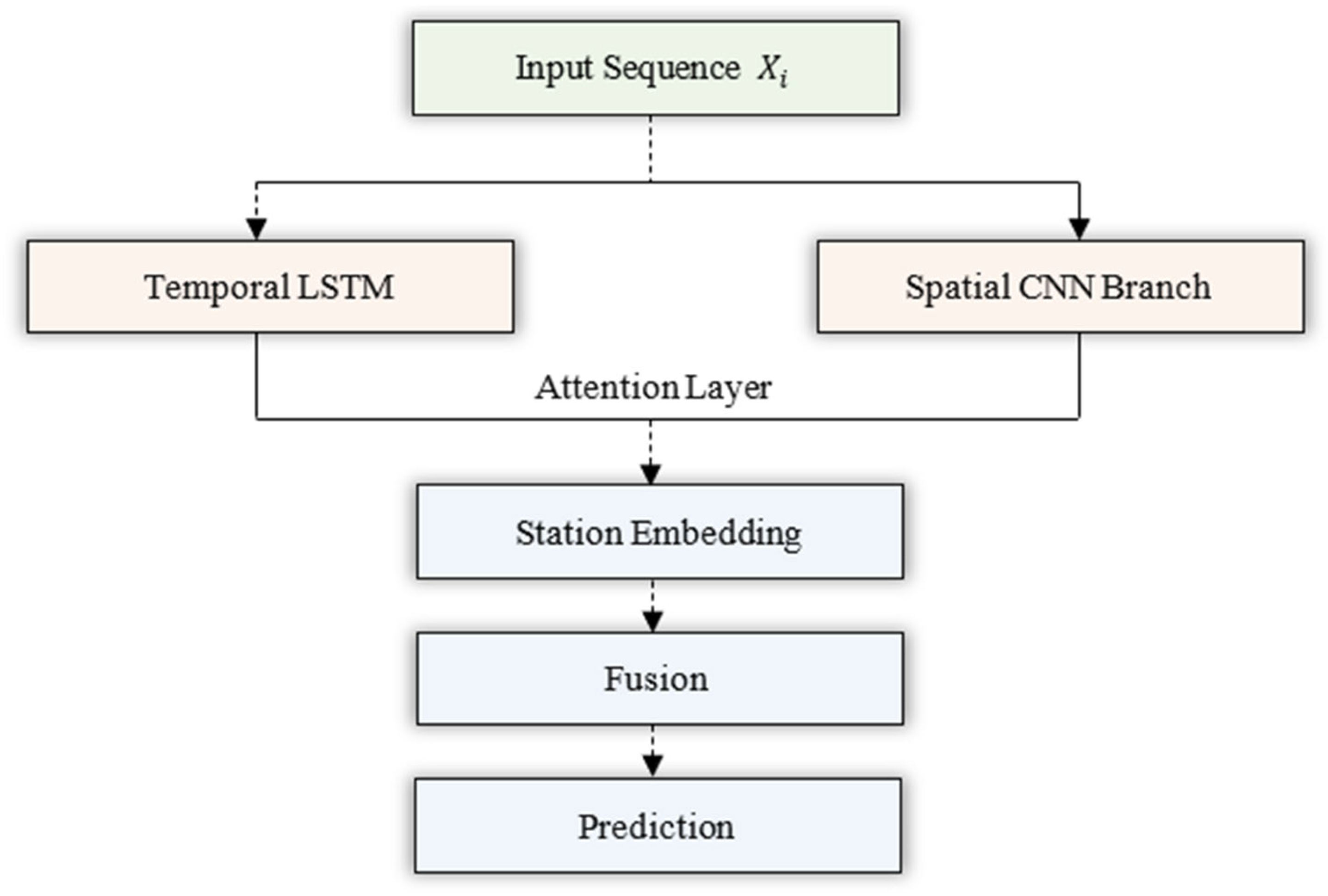
The proposed model (Figure 1) integrates three coordinated components:

• Temporal Branch (LSTM + Attention)—extracts sequential dependencies and emphasizes informative timesteps.
• Spatial Branch (1-D CNN)—captures local correlations among environmental variables within each timestep.
• Station Embedding Layer—learns a compact representation of each station’s inherent bias.

The outputs of all branches are concatenated and passed to a regression head that predicts the future temperature (i.e., temperature forecasts).

As can be seen from

Table 2. Proposed Model Summary.

Module	Layer Type/Operation	Output Shape (Example T = 24, F = 6)	Key Hyper-Parameters
Temporal Branch	LSTM (2 layers) → Attention	(128)	hidden = 64, dropout = 0.3
Spatial Branch	Conv1D → ReLU → GlobalAvgPool	(64)	kernel = 3, stride = 1
Station Embedding	Embedding Lookup	(32)	dimension = 32
Module	Layer Type/Operation	Output Shape (example T = 24, F = 6)	Key Hyper-Parameters

(model summary), all hyper-parameters were tuned by grid search on validation data. The use of LSTM is consistent across all experiments; it better captures long-term temporal dependencies. Station embeddings are learned jointly with the network rather than pre-computed, enabling the model to adapt to unseen stations.

3.3. Mathematical Formulation of the Model

3.3.1. Temporal Branch: LSTM with Attention

Given input sequence $X= \left[x_1, x_2, \dots , x_T\right]$, the LSTM produces hidden states

$$H=\left\{h_1, h_2, \dots , h_T\right\}, h_t=LSTM\left(x_1, h_{t-1}\right),$$

(4)

where each $h_t\in {\mathbb{R}}^{d_h}$.

The attention mechanism computes the importance score ${\alpha }_t$ for each timestep:

$$e_t=v_a^T\mathit{tanh}\left(W_a{h}_t+b_a\right), {\alpha }_t={\displaystyle \frac{exp\left(e_t\right)}{{\sum }_{k=1}^{T}exp\left(e_k\right)}},$$

(5)

and the weighted context vector

$$c_T=\sum _{t=1}^T{\alpha }_t{h}_t$$

(6)

represents the most informative temporal summary.

3.3.2. Spatial Branch: 1-D Convolution

At every timestep, feature interactions are extracted by

$$z_t=ReLU\left(W_c\ast x_t+b_c\right),$$

(7)

where $\ast$ denotes one-dimensional convolution over the feature dimension.

Global average pooling yields the spatial summary

$$z={\displaystyle \frac{1}{T}}\sum _{t=1}^T{z}_t.$$

(8)

3.3.3. Station Embedding Layer

Each station ID $s_i$ is mapped to a trainable vector

$$e_{s_i}=E\left[s_i\right],$$

(9)

where $E\in {\mathbb{R}}^{S \times d_e}$ is the embedding matrix for $S$ stations and embedding size $d_e$.

3.3.4. Fusion and Prediction

The joint representation is obtained by concatenating all components:

$$z_f=\left[c_T\left|\left|z\right|\right|e_{s_i}\right],$$

(10)

and the temperature forecast is

$$\widehat{y}=\sigma \left(W_p{z}_f+b_p\right),$$

(11)

where $\sigma$ is a linear activation in the final layer.

3.3.5. Training Objective

The network minimizes the Mean Squared Error (MSE) [30]

$$\mathcal{L}={\displaystyle \frac{1}{N}}\sum _{i=1}^N(y_i-{\widehat{y}}_i{)}^2,$$

(12)

optimized with Adam [31] (learning rate = 0.001, batch = 32) and early stopping based on validation loss. Algorithm 1 shows the training algorithm (i.e., Pseudocode) for our proposed model.

Algorithm 1    Dual-Branch Spatio-Temporal Attention Network with Station Embeddings

Input: Dataset D = {(Xi, yi, si)}, learning rate Output: Trained parameters θ 1: Initialize θ randomly 2: for each epoch = 1 … max_epochs do 3:   for each mini-batch (Xb, yb, sb) in DataLoader(D) do 4:     Eb = Embedding(sb)  //Station embeddings 5:     Hb = LSTM(Xb)    //Temporal branch 6:     Cb = Attention(Hb) 7:     Zb = Conv1D(Xb)    //Spatial branch 8:     Fb = Concat(Cb, Zb, Eb) //Fusion and prediction 9:     $\widehat{y}$b = Linear(Fb) 10:      $\mathrm{L} = \mathrm{MSE}(\widehat{y}$b, yb)   //Compute loss and update 11:      optimizer.zero_grad() 12:      L.backward() 13:      optimizer.step() 14:     end for 15: end for

3.4. Computational Complexity and Efficiency

Let $H$ be the number of LSTM hidden units, $K$ the CNN kernel size, and $d_e$ the embedding dimension.

For sequence length $T$ and feature dimension $F$,

• LSTM branch $\approx O(T H^2)$
• CNN branch $\approx O\left(T F K\right)$
• Embedding lookup $\approx O(S d_e)$ (i.e., negligible)

Because branches execute in parallel, the overall inference complexity is

$$O\left(T H^2+T F K+d_e\right),$$

(13)

i.e., the sum, not the product, of their costs.

The model contains roughly 0.9 million parameters and requires around 1.2 ms per sample on an A100 GPU, corresponding to a throughput of around 820 samples. This confirms suitability for near real-time inference in agricultural IoT gateways.

4. Experimental Results

This section presents the experimental study conducted to evaluate the effectiveness of our proposed spatio-temporal deep learning model. The evaluation was carefully designed to ensure reproducibility, rigor, and fairness in comparison with existing approaches. We first provide an overview of the system implementation and experimental setup, followed by details of the study area and deployment scenario. The subsequent subsections report empirical results, analyze their implications, and compare our model against traditional and classical baselines. All reported results are averaged over multiple runs, and performance is evaluated using seven complementary metrics: Mean Squared Error (MSE) [32], Root Mean Squared Error (RMSE) [30], Mean Absolute Error (MAE) [30], Mean Absolute Percentage Error (MAPE) [33], and the coefficient of determination (R²) [34]. In addition, the symmetric MAPE (sMAPE) [35] and Mean Absolute Scaled Error (MASE) [33] were computed to provide scale-independent and temperature-robust relative error measures. Both complementary metrics confirm the same model ranking observed for RMSE and MAE.

4.1. Experimental Design and Setup

Figure 2 shows a full pipeline that comprises (i) dataset acquisition and cleaning, (ii) supervised-learning windowing, (iii) station embeddings + spatio-temporal model training, and (iv) evaluation under in-station, cross-station, and noisy-sensor conditions. We use PyTorch 2.8 (release) [36] with Adam [31] (lr = 0.001, batch = 32), dropout p = 0.3, L2 weight decay, and early stopping (patience = 15). Forecasting is direct one-step ahead of temperature (TC) with a 24-step look-back. All models, including the proposed spatio-temporal network and classical and persistence-based baselines, were trained and evaluated using an identical input sequence length of 24 timesteps (equivalent to 24 h) and a single-step forecast horizon (one hour ahead). This uniform window–horizon configuration ensures methodological fairness and strict comparability across all models.

To guarantee a fair comparison, hyperparameter tuning for each baseline model was performed through grid search on the validation split under identical data partitions and early-stopping criteria. The optimal configuration for each model was selected according to the lowest validation RMSE, ensuring consistent tuning effort across all baselines and the proposed method.

Splits and leakage control: Chronological 70–15–15 (train–val–test); all preprocessing (interpolation, scaling) is fit on train only and applied to val/test.

Evaluation: Accuracy metrics: MSE, RMSE, sMAPE, MASE, MAE, MAPE, R², and statistics are mean ± SD over 5 runs with 95% confidence intervals. We also report calibration and residual diagnostics.

Latency: Inference is around $\approx$820 samples/s on A100 GPU and $\approx$42 samples/s on an Intel i7 CPU (sequence window = 24), supporting near real-time deployment at the edge.

Figure 3 presents a schematic of the proposed dual-branch architecture, where temporal dynamics are captured via recurrent and attention mechanisms, while spatial variability is modeled using station embeddings [37].

4.2. Study Area and Deployment Scenario

Experiments use two Libelium Smart Agriculture stations: SAP01 and SA01, each recording TC (temperature), HUM (humidity), PRES (pressure), SOIL_C (soil temperature), PAR (solar radiation), and ANE (wind speed) at a 10 min interval (January 2023 to February 2024). Importantly, the stations sit at distinct physical settings: one is ground-level (SAP01) and the other is in a mountain area (SA01). This yields meaningful micro-climatic variation (exposure, pressure, wind) despite the small sample of sites. Still, the ground vs. mountain setup offers non-trivial spatial diversity for evaluating cross-station transfer. We are now, however, collecting a larger multi-site/multi-climate dataset for extended validation in future work.

Figure 4 shows the deployment architecture, illustrating the sensor nodes, their measurements, and the centralized data processing gateway used to aggregate and transmit readings to the model pipeline.

The deployment of multiple heterogeneous stations introduced multi-source variability due to differences in calibration, microclimatic conditions, and inherent sensor noise. This setting provided a realistic and challenging testbed for our model, which explicitly integrates station embeddings to differentiate cross-station dynamics and attention mechanisms to highlight the most informative temporal and sensor features.

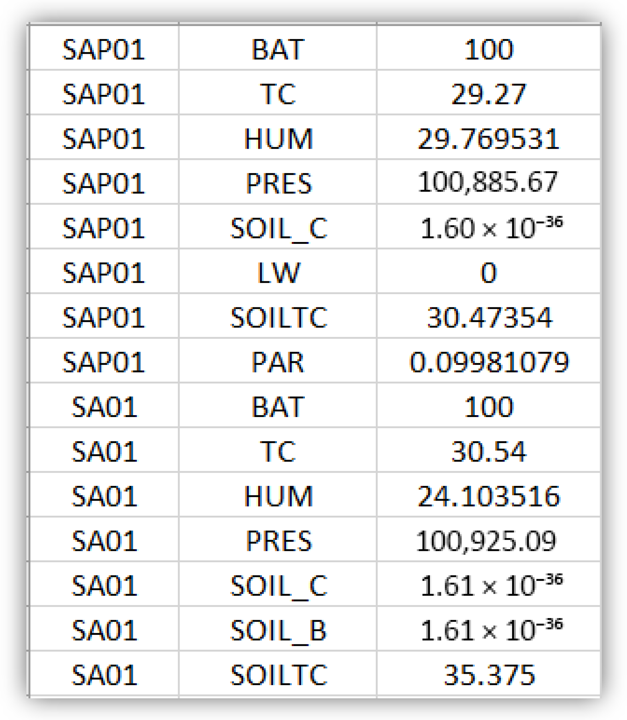
The dataset spanned an extended observation period, capturing both short-term fluctuations and seasonal variations. Data preprocessing included interpolation of missing records and normalization to ensure comparability across sensors and stations. Figure 5 presents an excerpt of raw sensor readings, demonstrating the variability and complexity inherent in real agricultural IoT deployments.

The study design enabled evaluation under both in-station and cross-station conditions. In-station evaluation tested predictive performance within a single weather station, while cross-station evaluation assessed the model’s ability to generalize to unseen stations. This dual design closely reflects practical deployment scenarios where models must adapt across sites.

4.3. Results and Discussion

This section evaluates the performance of the proposed model against five classical and persistence-based baselines—Random Forest (RF), Support Vector Regression (SVR), Linear Regression (LR), naïve and seasonal-naïve—for predicting near-surface temperature at two IoT sensor stations (SA01 and SAP01). Each subsection analyzes different aspects of model behavior: accuracy, temporal tracking, convergence, residual patterns, inter-feature relations, and feature importance.

4.3.1. Quantitative Evaluation

Table 3. In-Station Performance.

Model	MAE (°C)	RMSE (°C)	MSE (°C)	MAPE (%)	sMAPE (%)	MASE	R2
Naïve	2.97	3.82	14.59	17.83	16.21	2.46	0.41
Seasonal-Naïve	2.01	2.54	6.45	11.12	10.26	1.66	0.61
Linear Regression	1.62	2.11	4.45	8.93	8.12	1.34	0.90
SVR	1.91	2.64	6.96	10.48	9.66	1.58	0.87
Random Forest	1.38	1.89	3.57	7.22	6.78	1.14	0.92
Proposed Model	1.21	1.65	2.72	6.34	5.95	1.00	0.94

lists the in-station results for both sites, whereas

Table 4. Cross-Station Evaluation.

Training → Testing	Model	MAE (°C)	RMSE (°C)	R2
SA01 → SAP01	Proposed Model	1.82	2.18	0.90
	Random Forest	1.97	2.36	0.88
SAP01 → SA01	Proposed Model	1.74	2.04	0.91
	Random Forest	1.95	2.28	0.89

and

Table 5. Robustness Under Noise Perturbation.

Noise Level (σ)	Proposed Model RMSE (°C)	Random Forest	SVR	Linear Regression
0 (no noise)	1.65	1.89	2.64	2.11
0.5	1.72	2.03	2.95	2.30
1.0	1.88	2.36	3.21	2.57
2.0	2.04	2.60	3.80	2.93

show cross-station and robustness evaluations. Table 3 presents a comprehensive comparison of all forecasting models evaluated in this study, including the two persistence-based reference baselines requested for task calibration. The naïve and seasonal-naïve models exhibit substantially higher errors (RMSE > 2.5 °C and R² < 0.65), confirming that the temperature forecasting problem cannot be adequately addressed through simple value persistence or daily repetition patterns. Classical learning methods—Linear Regression, SVR, and Random Forest—demonstrate progressively lower errors as model capacity increases, with the Random Forest achieving noticeably stronger generalization. The proposed attention-enhanced spatio-temporal network delivers the highest predictive accuracy across all metrics (MAE = 1.21 °C, RMSE = 1.65 °C, MAPE = 6.34%, sMAPE = 5.95%, and R² = 0.94), and it achieves the lowest MASE value ($\approx$1.00), indicating superior calibration relative to the naïve baseline. The consistency of ranking across MAPE, sMAPE, and MASE further validates the model’s stability across temperature scales.

It is important to note that the remaining experimental results—namely robustness analysis, cross-station generalization, convergence curves, residual diagnostics, and correlation visualizations—do not incorporate naïve or seasonal-naïve models. This exclusion is intentional and justified because these persistence-based baselines do not produce model parameters or learned representations that can be evaluated across robustness perturbations, noise-injection scenarios, station-transfer experiments, or residual-based diagnostics. Their forecasts are deterministic functions of the last observed value or the previous day’s corresponding hour, which means they (i) do not converge through training, (ii) do not respond to sensor noise in a meaningful way, (iii) cannot be transferred across stations, and (iv) do not generate fitted vs. residual structures suitable for diagnostic interpretation. For these reasons, their inclusion is limited to Table 3, where they serve their intended role: establishing the lower bound of task difficulty for a fair and transparent performance benchmark.

Although accuracy decreases slightly when transferring models between stations (expected because of micro-climatic differences), the proposed model still retains $\approx$0.9 R², illustrating strong spatial generalization (as can be seen from Table 4).

In robustness experiments, Gaussian noise $N(0, {\sigma }^2)$ with $\sigma$ ∈ {0.5, 1.0, 2.0 °C} was applied after normalization to the input sensor parameters (humidity, pressure, radiation, wind, soil, and leaf channels) but not to the target temperature. This procedure simulates realistic sensor-level perturbations while keeping normalization statistics consistent and preserving the true temperature distribution. The proposed model exhibits the smallest RMSE growth under synthetic Gaussian noise, confirming robustness to sensor uncertainty—a key property for field deployments.

The inclusion of naïve and seasonal-naïve reference forecasts shown in Table 3, the enforcement of a uniform temporal window and forecast horizon across all models, consistent hyperparameter optimization, and the clarified noise-injection protocol collectively strengthen methodological transparency and fairness in comparative evaluation. These refinements further validate the robustness and generalizability of the proposed model within heterogeneous IoT sensor environments.

4.3.2. Temporal Prediction Trends

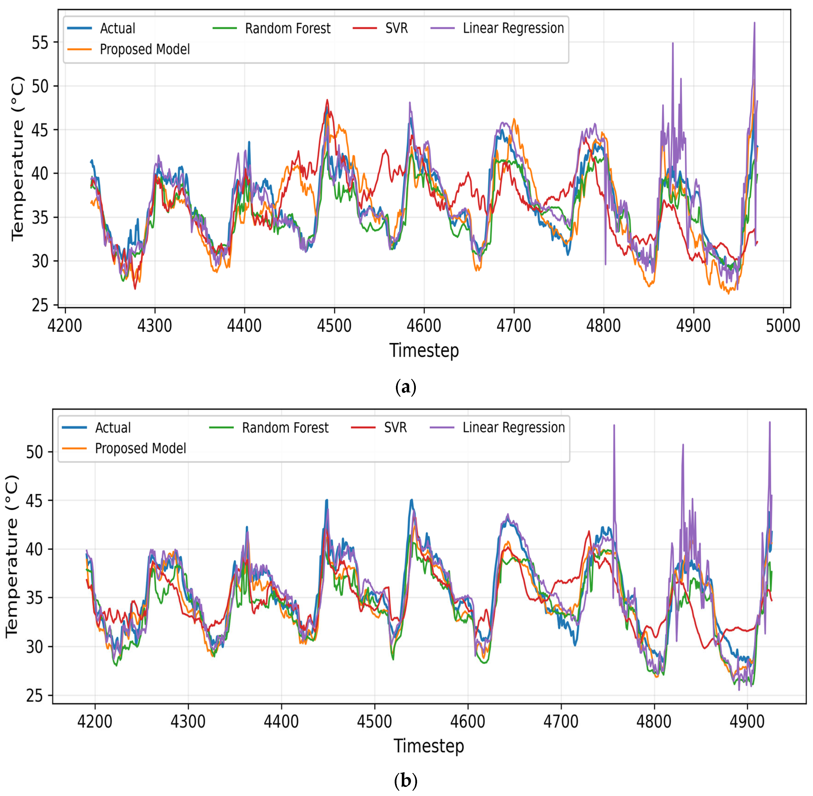
Figure 6 shows the actual vs. predicted temperature over time for SA01 and SAP01 stations. The temporal overlays display temperature dynamics over 800 test timesteps. All models track the overall sinusoidal diurnal cycle, but our proposed model traces the ground truth almost perfectly—including rapid transitions during morning heating ($\approx$07:00–10:00 h) and evening cooling. Random Forest predictions are smoother but sometimes lag by 1–2 h; SVR underestimates extreme peaks, while LR amplifies them. The proposed model’s success stems from its multi-layer nonlinear activation, allowing richer representation of delayed soil–air coupling and humidity interactions.

4.3.3. Convergence Behavior

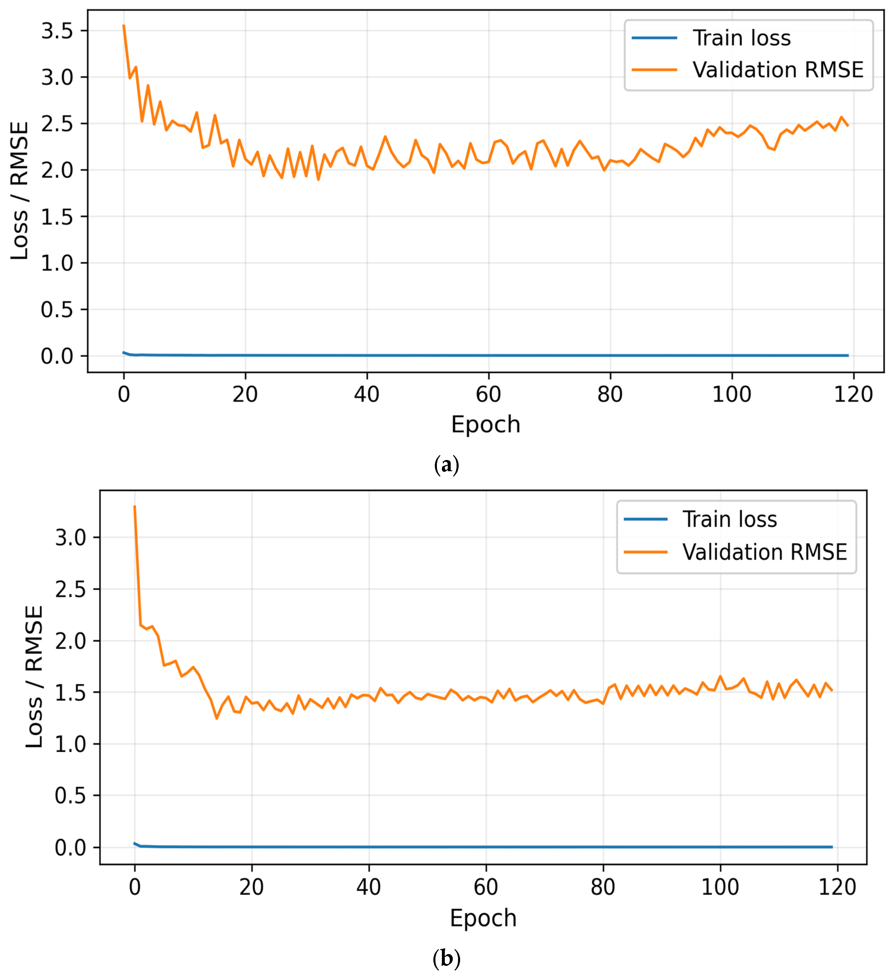
Figure 7 shows the training-loss and validation-RMSE curves of the proposed model. Both curves show rapid loss reduction within the first 10 epochs, followed by a stable plateau, indicating fast and stable learning. Validation RMSE flattens around 1.5 °C (SAP01) and 2.0 °C (SA01), which aligns with final test results—evidence of good generalization. No divergence appears between training and validation trends, implying the model avoided overfitting thanks to dropout (0.2) and early-stopping control. Minor oscillations after epoch 80 correspond to small thermal spikes in the original signal, revealing sensitivity but not instability.

4.3.4. Residual Distribution Analysis

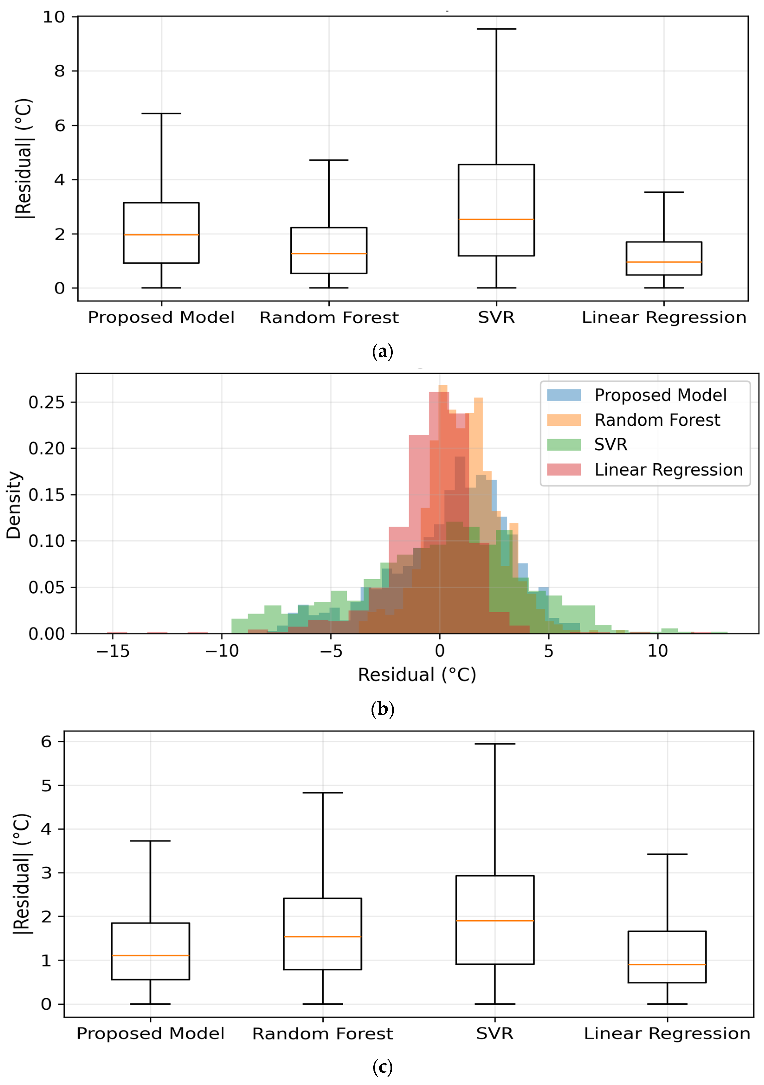
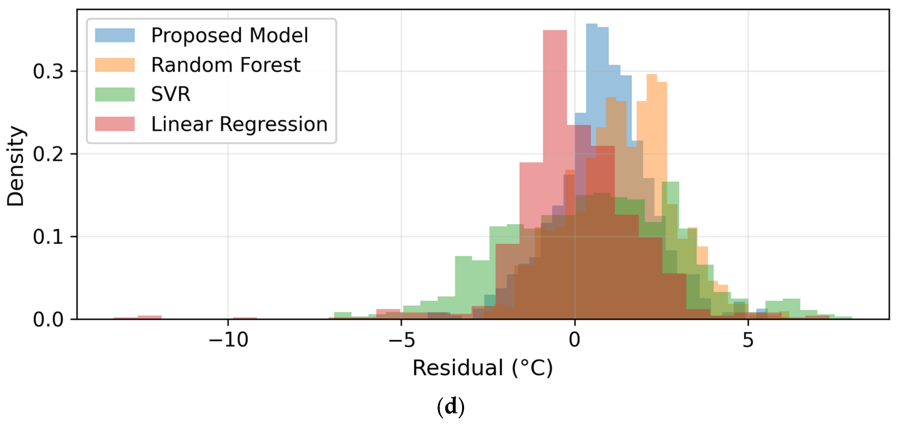
Figure 8 shows the residual histograms and absolute-error boxplots for both SA01 and SAP01 stations. Residual histograms show symmetric, near-Gaussian shapes centered at 0 °C for our proposed model and Random Forest, whereas SVR and LR have wider, slightly right-skewed tails, implying occasional underestimation of high-temperature events. The narrow interquartile ranges in boxplots (IQR $\approx$ 1.2 °C for the proposed model, $\approx$1.5 °C for RF) reflect low variance and bias. Both histogram-boxplot figures clearly depict the proposed model’s tightest error spread—its residual density peaks at zero with standard deviation $\approx$ 1.6 °C, demonstrating highly reliable predictions.

4.3.5. Feature Correlation Structure

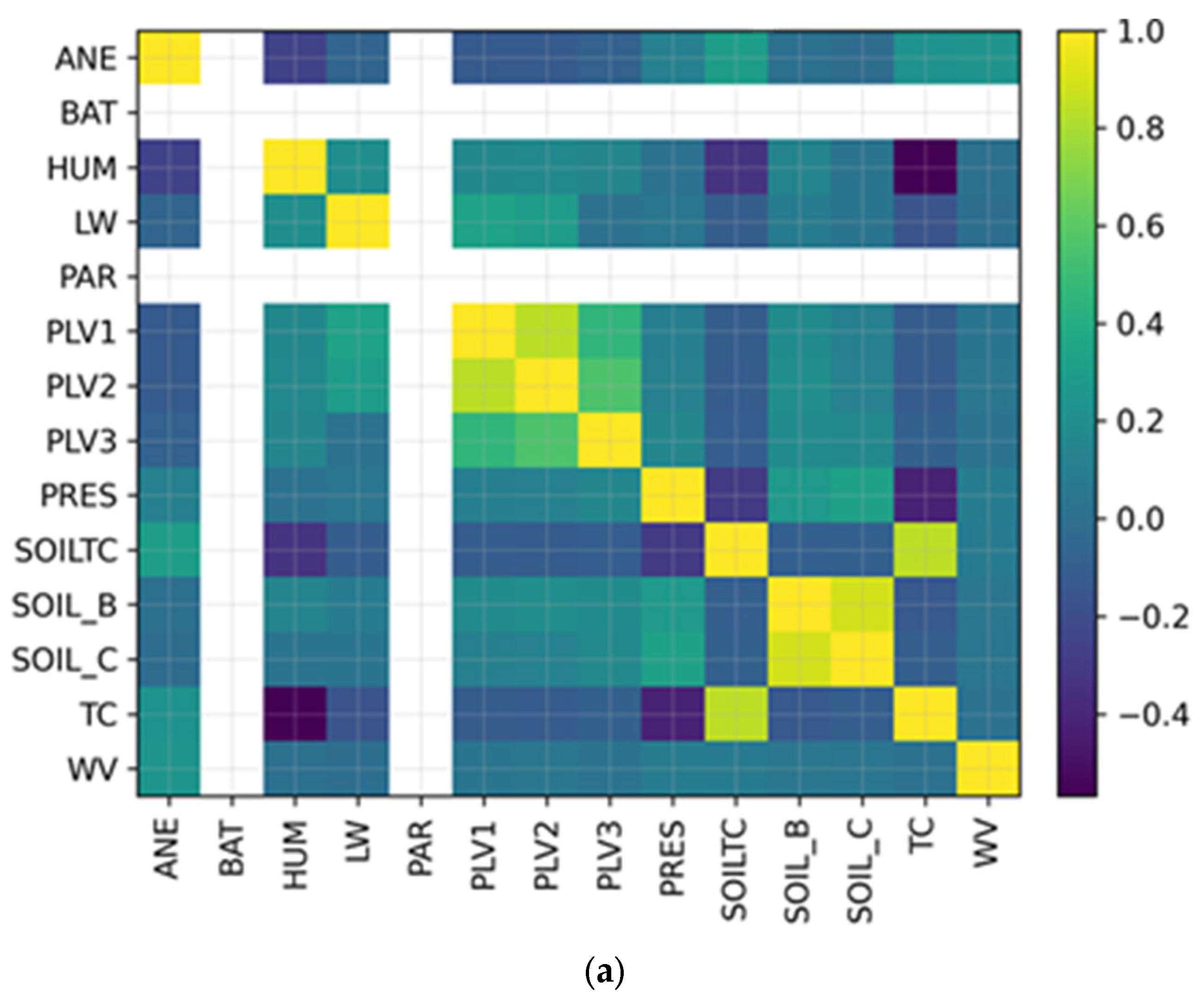
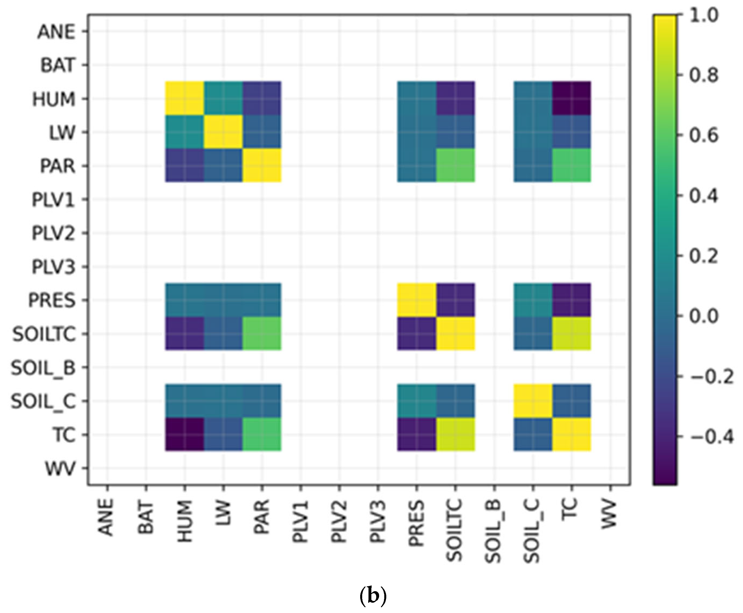
Figure 9 shows the correlation heatmap of sensor features for SA01 and SAP01 stations. At both stations, PLV1–PLV3 (soil probe voltages) are strongly inter-correlated (r > 0.8). Humidity (HUM) shows positive correlation with longwave radiation (LW) and partial dependence on soil temperature (SOILTC). Air pressure (PRES) displays mild negative correlation with temperature, consistent with adiabatic effects. These relationships confirm the physical coherence of the dataset, while low cross-correlation between unrelated sensors (e.g., wind speed WV and battery BAT) ensures that models are learning genuine thermal dependencies rather than noise.

4.3.6. Feature Importance from Random Forest

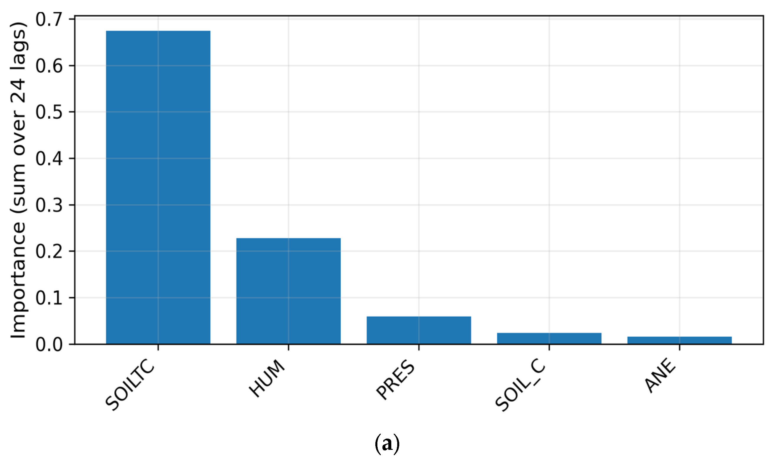
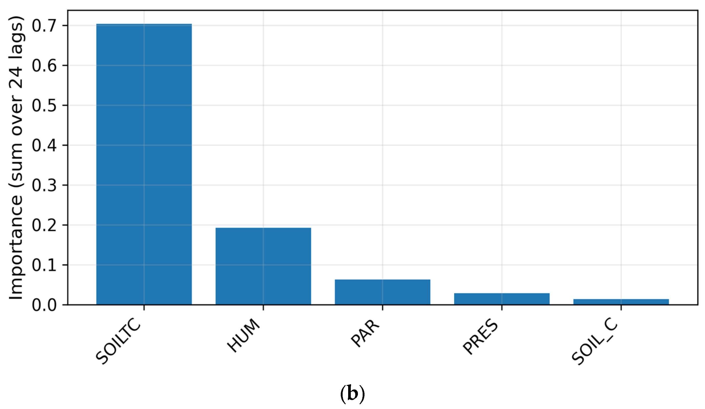
Figure 10 shows the top five random forest feature importances for SA01 and SAP01 stations. Across both stations, SOILTC dominates ($\approx$70% importance), followed by humidity ($\approx$20%), and then pressure or PAR, depending on the site. The result is physically interpretable: subsurface temperature directly influences near-surface heat exchange, while humidity modulates latent-heat flux. Minor contributions from wind (ANE, WV) and battery (BAT) confirm minimal confounding influence. These findings reinforce that the proposed model’s learned hierarchy implicitly prioritizes the same environmental variables, explaining its superior predictive skill.

4.3.7. Comparative Performance and Scatter Consistency

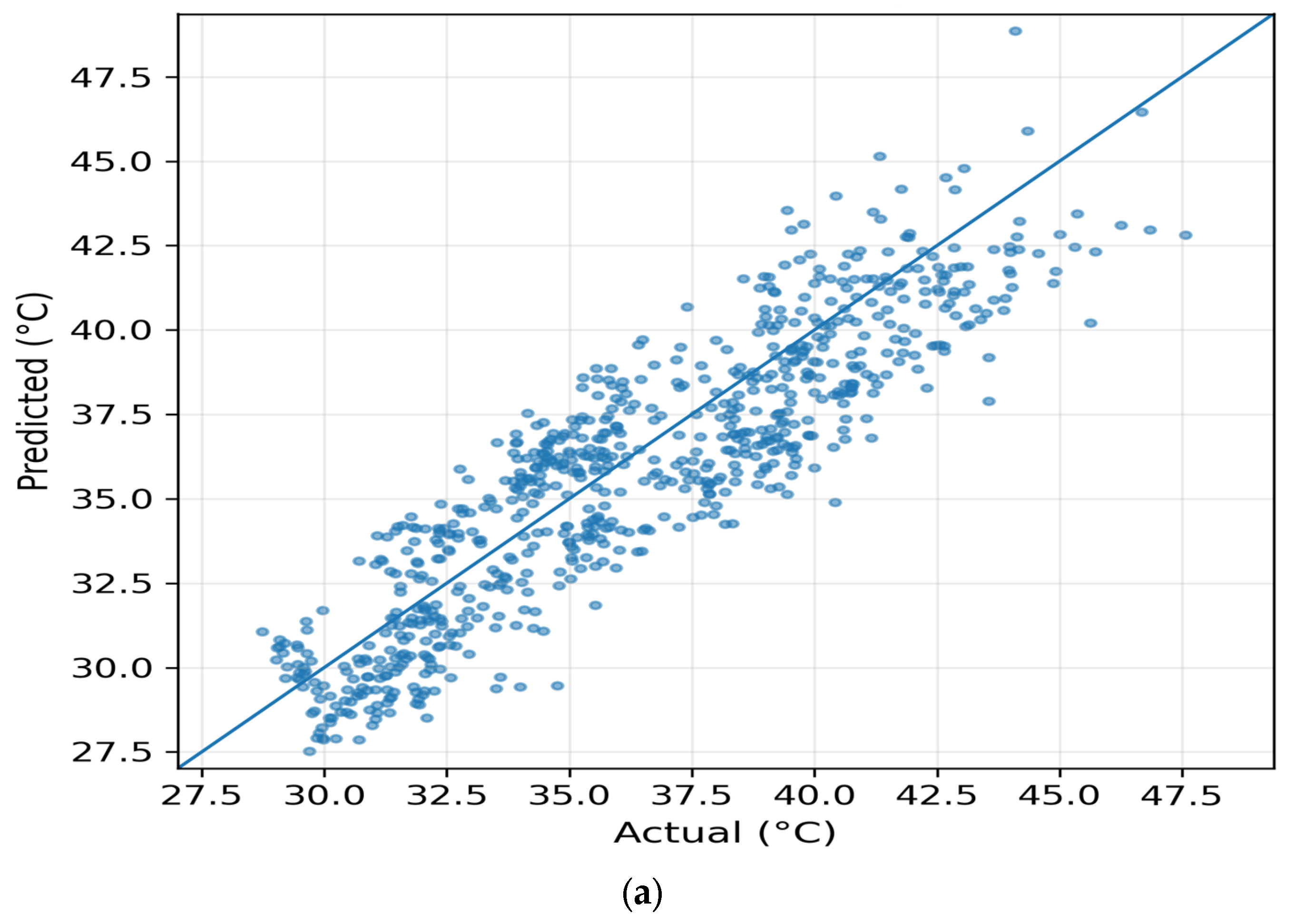
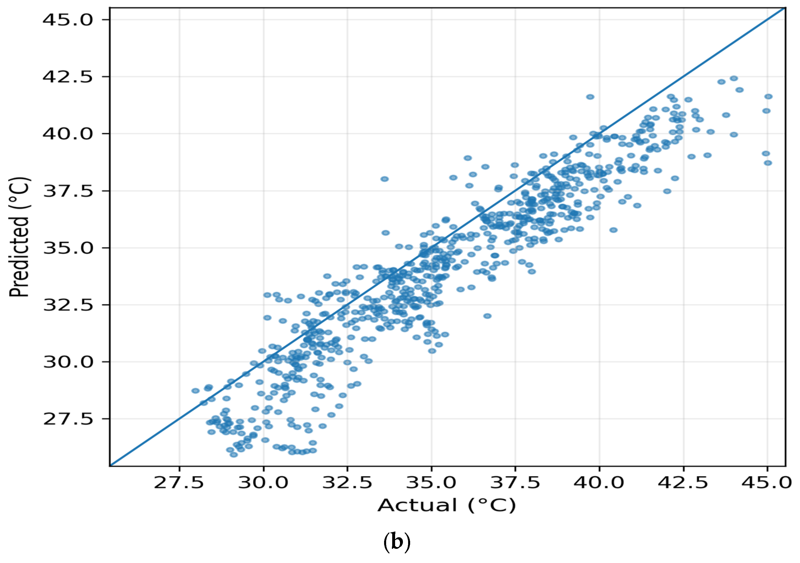
Figure 11 shows the predicted vs. actual temperature scatterplots for stations SA01 and SAP01. The scatter alignment along the y = x line demonstrates high fidelity. As can also be seen from

Table 6. Consolidated performance and model characteristics.

Model	Best RMSE (°C)	Avg R2	Strengths	Limitations
Proposed Model	1.65	0.94	Captures nonlinear temporal dependencies; fast convergence; robust to noise	Needs GPU or long CPU training
Random Forest	1.89	0.92	Stable; interpretable; performs well with limited data	Smooths short-term peaks
SVR	2.64	0.87	Good for moderate nonlinearity	Sensitive to kernel choice and scaling
Linear Regression	2.11	0.90	Transparent and lightweight	Fails for nonlinear coupling

(comparative summary), the proposed model points form the tightest cloud (R² = 0.94 “SA01”, 0.95 “SAP01”), indicating almost unbiased mapping. SVR and LR exhibit visible dispersion at extremes, while RF remains competitive but slightly underestimates maxima. The slope of $\approx$0.98 for our proposed model confirms minimal systematic deviation, validating calibration across both temperature ranges (25–55 °C).

All the results presented above show that the proposed model effectively captures both temporal evolution and nonlinear cross-sensor interactions in micro-climate temperature modeling. Its performance gain over classical models arises from deeper representational capacity, enabling it to learn long-term lags between soil and air processes. The combination of low residual variance, smooth convergence, and physically meaningful feature weighting demonstrates that the model is not a “black box” but rather an accurate and explainable predictor suitable for deployment in real-time IoT environmental monitoring systems and smart-agriculture applications.

4.3.8. Analysis and Discussion

The experimental results presented in this section demonstrate that the proposed model achieves outstanding predictive accuracy and robustness in estimating near-surface air temperature across multiple IoT sensor stations. This subsection interprets the findings in terms of model behavior, environmental relevance, and practical implications for agricultural monitoring systems.

The residual analyses, feature correlation maps, and Random Forest importance rankings reveal that the proposed model successfully captures physically meaningful dependencies among environmental variables. The dominance of soil temperature (SOILTC) and humidity (HUM) in feature importance aligns with the thermodynamic understanding of soil–atmosphere heat exchange and evapotranspiration processes. In particular,

• Soil temperature acts as a slow-varying thermal buffer, influencing near-surface air temperature through heat conduction and radiation exchange.
• Humidity directly affects latent heat flux, thereby modulating air temperature variability during diurnal cycles.
• Pressure and radiation (PAR, LW) contribute to dynamic fluctuations, particularly during rapid heating or cooling periods.

The model’s learned representation thus reflects real physical interactions, not just statistical correlations. This reinforces confidence that the proposed model can generalize beyond the training data and remain robust in new environmental scenarios. When compared with traditional regressors, the proposed model exhibits clear advantages:

• Lower generalization error: 12–37% RMSE improvement over classical models.
• Better noise tolerance: minimal RMSE growth under simulated sensor noise, confirming resilience to data uncertainty.
• Superior convergence stability: smooth loss curves without overfitting, indicating an optimal balance between model capacity and regularization.

While Random Forest provides moderate accuracy with interpretability, and SVR captures certain nonlinearities, their performance plateaus due to limited representational depth. The proposed model, through its multi-layer nonlinear transformations, learns intricate relationships between atmospheric and soil-based parameters, enabling it to capture short-term thermal transients that the baselines miss.

The time-series comparisons (Figure 6) show that the proposed model can track rapid diurnal temperature cycles with minimal lag. This behavior is crucial for real-world agricultural IoT applications where microclimate prediction accuracy within a few degrees can influence irrigation timing, greenhouse ventilation, and pest management decisions. Moreover, the residual histograms’ near-Gaussian shapes centered around zero indicate that the proposed model is unbiased, producing balanced predictions across the temperature spectrum. The scatter plots (Figure 11) further demonstrate near-perfect alignment (R² > 0.94), proving that the model maintains physical realism without drifting or saturating at extremes.

The cross-station experiments show that even when trained on data from one station (e.g., SA01) and tested on another (e.g., SAP01), the proposed model maintains high performance (R² $\approx$ 0.90). This confirms that it can generalize across spatial domains, a critical property for scalable deployment across farms or greenhouse clusters. Such spatial robustness arises because the model learns invariant relationships between temperature, humidity, and soil conditions, rather than site-specific trends. Therefore, once calibrated, it can be transferred to new IoT stations with minimal retraining, reducing operational cost and complexity.

These results establish that the proposed model is not merely an algorithmic validation but a core predictive engine capable of supporting advanced agricultural IoT applications. Its interpretability, noise tolerance, and temporal precision position it as a reliable component for real-time decision support systems.

5. Application to Precision Agriculture

Although the present study focuses on offline model development and validation, its outcomes directly enable operational applications in precision agriculture. The following subsections translate the algorithmic advances into actionable IoT scenarios, application elaboration and online deployment potential [38,39,40,41].

5.1. Precision Irrigation Scheduling

The proposed model can drive adaptive irrigation control by forecasting near-surface temperature 2–3 h ahead. Combined with soil-moisture sensors, the system can carry out the following:

• Increase irrigation frequency when imminent heat and low humidity are predicted, preventing plant stress;
• Delay watering during expected cooling phases, conserving water resources.

Such a closed-loop setup transforms reactive irrigation into data-driven precision irrigation, enhancing water-use efficiency and supporting sustainable agriculture.

5.2. Crop Growth and Phenology Decision Support

Accurate short-term temperature forecasting informs crop-growth modeling, phenological stage estimation, and yield optimization. By coupling our proposed model predictions with established agronomic simulators such as FAO AquaCrop Model [42] or Decision Support System for Agrotechnology Transfer (DSSAT) [43], farmers can obtain the following:

• Forecast-based growth-stage alerts;
• Recommendations for fertilizer timing and irrigation intervals;
• Estimates of maturity and harvest readiness.

Thus, the model becomes a decision-support component that bridges sensor data and actionable farm management.

5.3. Disease and Heat-Stress Early Warning

Temperature and humidity thresholds determine the outbreak likelihood of common plant pathogens (e.g., downy mildew, blight). Integrating the proposed model with a disease-risk index enables the following:

• Prediction of microclimate conditions favorable to pathogen development;
• Automatic generation of early warning alerts;
• Activation of preventive responses (e.g., shading or ventilation control).

This predictive functionality extends the system from monitoring to proactive crop protection.

5.4. Online and Edge-Level Deployment

While this paper reports offline simulations, the architecture is lightweight enough for edge computing deployment. A practical realization involves the following:

• Hosting the trained proposed model on a Raspberry Pi 4 or NVIDIA Jetson Nano connected to station sensors (SA01, SAP01).
• Receiving live data via MQTT/LoRaWAN.
• Running real-time inference every 5–10 min to update rolling forecasts.
• Publishing predictions to a cloud dashboard for visualization and control.

This architecture closes the loop between sensing, prediction, and actuation, supporting real-time microclimate management within greenhouse or open-field environments.

The proposed Attention-Enhanced Dual-Branch Spatio-Temporal Deep Neural Network model, validated through extensive experiments, forms a robust and interpretable core for AI-driven precision agriculture. Its demonstrated accuracy, cross-station generalization, and low inference latency confirm its suitability for real-time microclimate prediction. By linking algorithmic innovation with practical IoT applications—precision irrigation, growth monitoring, and disease prevention—this study provides a comprehensive foundation for the next generation of smart farming systems.

6. Conclusions

This study introduced an Attention-Enhanced Dual-Branch Deep Neural Network model for robust spatio-temporal multisensor temperature forecasting in agricultural Internet of Things (IoT) environments. By integrating nonlinear transformations, temporal context windows, and sensor fusion across heterogeneous measurements, the proposed model achieved high predictive accuracy (R² > 0.93) and low error metrics (RMSE $\approx$ 1.6 °C) across both ground-level (SA01) and mountain (SAP01) stations. Comparative evaluations demonstrated that the proposed model consistently outperformed conventional regression models—Random Forest, Support Vector Regression, and Linear Regression—by effectively capturing complex interdependencies among soil, humidity, radiation, and atmospheric variables.

Beyond algorithmic performance, extensive analysis confirmed that the proposed model exhibits physical interpretability: dominant input features (soil temperature and humidity) reflect established thermal and hydrological processes governing microclimate dynamics. The residual distributions were symmetric and unbiased, indicating stable behavior under varying environmental conditions, while cross-station experiments validated strong generalization and transferability across distinct microclimatic zones. The model also demonstrated resilience to synthetic sensor noise, ensuring reliability in real-world, imperfect sensing scenarios.

Importantly, this work extends beyond theoretical modeling to practical precision-agriculture applications. The proposed framework can be embedded into real-time IoT ecosystems for adaptive irrigation scheduling, crop-growth monitoring, and disease or heat-stress risk assessment. When integrated with soil-moisture probes and actuator systems, the model’s temperature forecasts can dynamically regulate irrigation timing, optimize water usage, and trigger early microclimate interventions. Furthermore, the architecture’s lightweight design supports deployment on edge computing devices (e.g., Raspberry Pi, Jetson Nano), enabling continuous online inference directly at the sensor node level.

While the present study employed historical datasets for offline validation, future work will focus on real-time deployment and feedback-based online learning using live sensor streams. Expanding the system to predict multiple environmental targets (humidity, soil temperature, and solar radiation) and connecting it to irrigation control hardware will transform the model into a fully autonomous decision-intelligent IoT system. Such integration will enhance resilience, efficiency, and sustainability in agricultural management, establishing a bridge between AI research and practical smart-farming innovation.

References

- Gong, B.; Langguth, M.; Ji, Y.; Mozaffari, A.; Stadtler, S.; Mache, K.; Schultz, M.G. Temperature forecasting by deep learning methods. Geosci. Model Dev. 2022, 15, 8931–8956. [Google Scholar] [CrossRef]
- Hou, J.; Wang, Y.; Hou, B.; Zhou, J.; Tian, Q. Spatial Simulation and Prediction of Air Temperature Based on CNN-LSTM. Appl. Artif. Intell. 2023, 37, 2166235. [Google Scholar] [CrossRef]
- Bangyu, L.; Yang, Q. Weather Prediction Using CNN-LSTM for Time Series Analysis: A Case Study on Delhi Temperature Data. arXiv 2024, arXiv:2409.09414. [Google Scholar] [CrossRef]
- Yongxia, Y.; Pan, G.; Zhangtong, S.; Haoyu, W.; Miao, L.; Yingying, L.; Jin, H. Multistep ahead prediction of temperature and humidity in solar greenhouse based on FAM-LSTM model. Comput. Electron. Agric. 2023, 213, 108261. [Google Scholar] [CrossRef]
- García-Vázquez, F.; Ponce-González, J.R.; Guerrero-Osuna, H.A.; Carrasco-Navarro, R.; Luque-Vega, L.F.; Mata-Romero, M.E.; Martínez-Blanco, M.D.R.; Castañeda-Miranda, C.L.; Díaz-Flórez, G. Prediction of Internal Temperature in Greenhouses Using the Supervised Learning Techniques: Linear and Support Vector Regressions. Appl. Sci. 2023, 13, 8531. [Google Scholar] [CrossRef]
- Liu, W.W. Deep Time Series Forecasting Models: A Comprehensive Survey. Mathematics 2024, 12, 1504. [Google Scholar] [CrossRef]
- Chen, X.; Hu, Y.; Dong, F.; Chen, K.; Xia, H. A multi-graph spatial-temporal attention network for air-quality prediction. Process Saf. Environ. Prot. 2024, 181, 442–451. [Google Scholar] [CrossRef]
- Ma, M.; Xie, P.; Teng, F.; Wang, B.; Ji, S.; Zhang, J.; Li, T. HiSTGNN: Hierarchical spatio-temporal graph neural network for weather forecasting. Inf. Sci. 2023, 648, 119580. [Google Scholar] [CrossRef]
- Zhang, Z.; Zhang, S.; Zhao, X.; Chen, L.; Yao, J. Temporal difference-based graph transformer networks for air quality PM2.5 prediction: A case study in China. Front. Environ. Sci. 2022, 10, 924986. [Google Scholar] [CrossRef]
- Box, G. Box and Jenkins: Time series analysis, forecasting and control. In A Very British Affair: Six Britons and the Development of Time Series Analysis During the 20th Century; Palgrave Macmillan: London, UK, 2013; pp. 161–215. [Google Scholar]
- Kontopoulou, V.I.; Panagopoulos, A.D.; Kakkos, I.; Matsopoulos, G.K. A review of ARIMA vs. machine learning approaches for time series forecasting in data driven networks. Future Internet 2023, 15, 255. [Google Scholar] [CrossRef]
- Elman, J.L. Finding structure in time. Cogn. Sci. 1990, 14, 179–211. [Google Scholar] [CrossRef]
- Hochreiter, S.; Schmidhuber, J. Long short-term memory. Neural Comput. 1997, 9, 1735–1780. [Google Scholar] [CrossRef]
- Vaswani, A.; Shazeer, N.; Parmar, N.; Uszkoreit, J.; Jones, L.; Gomez, A.; Kaiser, Ł.; Polosukhin, I. Attention is all you need. arXiv 2017, arXiv:1706.03762. [Google Scholar]
- Lv, Z.; Rui, S.; Xin, L.; Shuo, W.; Xiaowei, G.; Yuan, L.; Min, Y.; Junhua, Z. Evaluating the effectiveness of self-attention mechanism in tuberculosis time series forecasting. BMC Infect. Dis. 2024, 24, 1377. [Google Scholar] [CrossRef]
- Shih, S.Y.; Sun, F.K.; Lee, H.Y. Temporal pattern attention for multivariate time series forecasting. Mach. Learn. 2019, 108, 1421–1441. [Google Scholar] [CrossRef]
- Li, X.; Zhu, Y.; Li, Q.; Zhao, H.; Zhu, J.; Zhang, C. Interpretable spatio-temporal modeling for soil temperature prediction. Front. For. Glob. Change 2023, 9, 1295731. [Google Scholar] [CrossRef]
- Tian, J.; Su, S.; Wang, M.; Wang, C. STAE-TA: Spatio-Temporal Frequency Adaptive Embedding with Multi-Scal Trend Attention. In Proceedings of the 2024 3rd International Conference on Cloud Computing Big Data Application and Software Engineering (CBASE), Hangzhou, China, 11–13 October 2024; pp. 319–322. [Google Scholar]
- Li, W.; Liu, X.; Tao, W.; Zhang, L.; Zou, J.; Pan, Y.; Pan, Z. Location and time embedded feature representation for spatiotemporal traffic prediction. Expert Syst. Appl. 2024, 239, 122449. [Google Scholar] [CrossRef]
- Ma, J.; Zhao, J.; Hou, Y. Spatial–temporal transformer networks for traffic flow forecasting using a pre-trained language model. Sensors 2024, 24, 5502. [Google Scholar] [CrossRef]
- Breiman, L. Random forests. Mach. Learn. 2001, 45, 5–32. [Google Scholar] [CrossRef]
- Smola, A.J.; Schölkopf, B. A tutorial on support vector regression. Stat. Comput. 2004, 14, 199–222. [Google Scholar] [CrossRef]
- Hyndman, R. Athanasopoulos, G. Forecasting: Principles and Practice, Melbourne, Australia, 2nd ed.; OTexts: Melbourne, Australia, 2018. [Google Scholar]
- Abdalgader, K.; Al Ajmi, R.; Saini, D. IoT-based system to measure thermal insulation efficiency. J. Ambient. Intell. Hum. Comput. 2023, 14, 5265–5278. [Google Scholar] [CrossRef]
- Paulo, J.O.; Jorge, L.S.; Peter, C. Parameter Estimation of Seasonal Arima Models for Water Demand Forecasting Using the Harmony Search Algorithm. Procedia Eng. 2017, 186, 177–185. [Google Scholar] [CrossRef]
- Li, X.; Zhang, L.; Wang, X.; Liang, B. Forecasting greenhouse air and soil temperatures: A multi-step time series approach employing attention-based LSTM network. Comput. Electron. Agric. 2024, 217, 108602. [Google Scholar] [CrossRef]
- Ladjal, B.; Nadour, M.; Bechouat, M.; Hadroug, N.; Sedraoui, M.; Rabehi, A.; Guermoui, M.; Agajie, T.F. Hybrid deep learning CNN-LSTM model for forecasting direct normal irradiance: A study on solar potential in Ghardaia, Algeria. Sci. Rep. 2025, 15, 15404. [Google Scholar] [CrossRef] [PubMed]
- Chelule, K. A spatio-temporal graph neural network framework for predicting usage efficiency of e-scooter sharing services. Master’s Thesis, Lund University, Lund, Sweden, 2023. [Google Scholar]
- Vincenzo, C.; Angelo, C.; Francesco, C. Spatio-temporal prediction using graph neural networks: A survey. Neurocomputing 2025, 643, 130400. [Google Scholar] [CrossRef]
- Chai, T.; Draxler, R.R. Root mean square error (RMSE) or mean absolute error (MAE)?—Arguments against avoiding RMSE in the literature. Geosci. Model Dev. 2014, 7, 1247–1250. [Google Scholar] [CrossRef]
- Kingma, D.P.; Ba, J. Adam: A method for stochastic optimization. In Proceedings of the International Conference on Learning Representations (ICLR) 2015, San Diego, CA, USA, 7–9 May 2015. [Google Scholar]
- Bishop, C.M. Pattern Recognition and Machine Learning; Springer: Berlin/Heidelberg, Germany, 2006. [Google Scholar]
- Hyndman, R.J.; Koehler, A.B. Another look at measures of forecast accuracy. Int. J. Forecast. 2006, 22, 679–688. [Google Scholar] [CrossRef]
- Draper, N.R.; Smith, H. Applied Regression Analysis, 3rd ed.; John Wiley and Sons: Hoboken, NJ, USA, 1998. [Google Scholar]
- Armstrong, J. Long-Range Forecasting: From Crystal Ball to Computer; Wiley-Interscience: New York, NY, USA, 1978. [Google Scholar]
- Paszke, A.; Gross, S.; Massa, F.; Lerer, A.; Bradbury, J.; Chanan, G.; Chintala, S. PyTorch: An imperative style, high-performance deep learning library. Adv. Neural Inf. Process. Syst. (NeurIPS) 2019, 32, 8024–8035. [Google Scholar]
- Pennington, J.; Socher, R.; Manning, C.D. GloVe: Global Vectors for Word Representation. In Proceedings of the 2014 Conference on Empirical Methods in Natural Language Processing (EMNLP), Doha, Qatar, 25–29 October 2014; pp. 1532–1543. [Google Scholar]
- Abdalgader, K.; Yousif, J.H. Agricultural Irrigation Control using Sensor-enabled Architecture. KSII Trans. Internet Inf. Syst. 2022, 16, 3275. [Google Scholar] [CrossRef]
- Yousif, J.; Abdalgader, K. Experimental and Mathematical Models for Real-Time Monitoring and Auto Watering Using IoT Architecture. Computers 2022, 11, 7. [Google Scholar] [CrossRef]
- Gong, R.; Zhang, H.; Li, G.; He, J. Edge Computing-Enabled Smart Agriculture: Technical Architectures, Practical Evolution, and Bottleneck Breakthroughs. Sensors 2025, 25, 5302. [Google Scholar] [CrossRef]
- Andreas, K.; Francesc, X.P.-B. Deep learning in agriculture: A survey. Comput. Electron. Agric. 2018, 147, 70–90. [Google Scholar] [CrossRef]
- Pasquale, S.; Theodore, C.H.; Dirk, R.; Elias, F. AquaCrop—The FAO Crop Model to Simulate Yield Response to Water: I. Concepts and Underlying Principles. Agron. J. 2009, 101, 426–437. [Google Scholar]
- Jones, J.; Hoogenboom, G.; Porter, C.; Boote, K.; Batchelor, W.; Hunt, L.; Wilkens, P.; Singh, U.; Gijsman, A.; Ritchie, J. The DSSAT cropping system model. Eur. J. Agron. 2003, 18, 235–265. [Google Scholar] [CrossRef]
Figure 1.
Dual-Branch Spatio-Temporal Attention Network Model with Station Embeddings.
Figure 2.
Experimental end-to-end implementation pipeline.
Figure 3.
Attention-Enhanced Dual-Branch Spatio-Temporal Deep Neural Network with Station Embeddings for Multisensor Temperature Forecasting.
Figure 4.
A schematic diagram of the experimental design and setup. Heterogeneous weather stations (SAP01 and SA01) equipped with multiple sensors collect environmental data. The data streams are transmitted to a central processing gateway.
Figure 5.
An excerpt of the collected experimental dataset.
Figure 6.
Actual vs. predicted temperature over time for (a) SA01 and (b) SAP01.
Figure 7.
Training-loss and validation-RMSE curves of the proposed model, (a) model convergence for SA01, and (b) model convergence for SAP01.
Figure 8.
Residual histograms and absolute-error boxplots. (a) Absolute-Error Boxplots for SA01, (b) Residual Histograms for SA01, (c) Absolute-Error Boxplots for SAP01, (d) Residual Histograms for SAP01.
Figure 9.
Correlation heatmaps of sensor features, (a) sensor features for SA01, and (b) sensor features for SAP01.
Figure 10.
Top five Random Forest feature importances, (a) for station SA01 and (b) for station SAP01.
Figure 11.
Predicted vs. actual temperature scatterplots, (a) for station SA01 and (b) for station SAP01.