Abstract
Most fruit classification studies rely on color-based features, but shape-based analysis provides a promising alternative for distinguishing subtle variations within the same variety. Tomato shape classification is challenging due to irregular contours, variable imaging conditions, and difficulty in extracting consistent geometric features. In this study, we propose an efficient and structured workflow to address these challenges through contour-based analysis. The process begins with the application of a Mask Region-based Convolutional Neural Network (Mask R-CNN) model to accurately isolate tomatoes from the background. Subsequently, the segmented tomatoes are extracted and encoded using Elliptic Fourier Descriptors (EFDs) to capture detailed shape characteristics. These features are used to train a range of machine learning models, including Support Vector Machine (SVM), Random Forest, One-Dimensional Convolutional Neural Network (1D-CNN), and Bidirectional Encoder Representations from Transformers (BERT). Experimental results observe that the Random Forest model achieved the highest accuracy of 79.4%. This approach offers a robust, interpretable, and quantitative framework for tomato shape classification, reducing manual labor and supporting practical agricultural applications.
1. Introduction
Recognizing fruits, shapes, colors, and weight are some of the essential characteristics. Different features may represent distinct crop varieties and sometimes even indicate the quality of the fruits. For instance, tomatoes having diverse shapes may be needed in disparate uses, depending on whether they are process-type tomatoes or fresh-type tomatoes [1], which also affects the commercial values. In Taiwan, tomatoes are one of the all-time favorite kinds of fruits that attract customers, and one of the unique varieties is named “Cherry Tomato.” Its high sweetness level and its great texture appeal to customers, thus bringing huge profits to the cherry tomato farmers. More and more growers tend to join the trend of planting this kind of tomato. By differentiating the appearance of the tomatoes, fruits with rather attractive shapes tend to be more profitable. However, identifying the patterns of tomatoes to determine the higher sale-price ones is labor-intensive and time-consuming. Due to the high economic value of cherry tomatoes, we aim to develop a classification model for sorting cherry tomatoes based on the shape of the bottom part of the tomatoes to reduce the work effort and increase effectiveness.
Image processing and machine learning techniques have been used in identifying different kinds of vegetables and fruits in the past few years. Most of them focused on detecting the color of the crops since it is the first characteristic that comes into sight. Hossain et al. [2] built an automatic fruit classification system with a deep learning framework. These sorts of systems can be employed in identifying fruit species and help specify the crops’ ripeness, or check if there are diseases. Others emphasize the shape and contours of the fruits. These shape-oriented models are valuable when the detection goal is to distinguish diverse types of the same variety of fruit, since they may not have observable color differences. Plenty of features can be extracted and analyzed, so it is crucial to select the representative ones. Ishikawa et al. [3] tried several strawberry descriptors, including Ellipse Similarity Index (ESI), Elliptic Fourier Descriptors (EFDs), Chain Code Subtraction (CCS), and other measured values (MVs) like widths and lengths to find a combination that brings out the highest accuracy classification. Furthermore, they eventually discovered that using MVs + CCS + EFD achieves their goal. In order to acquire the fruits’ characters, some studies exploited Tomato Analyzer (v2.2) [4,5,6], a software that helps quantify fruits’ morphology and color data. The program provides more objective and precise data than the manually collected ones. Visa et al. [7] used Tomato Analyzer to collect contour morphometric data from images. After that, they implemented unsupervised learning techniques and meta-clustering to classify tomato fruits. Other studies, such as Sharma et al. [8] used HOG descriptors to extract descriptors from carrots, obtaining histograms of oriented gradients and testing by KNN, K-Fold Cross-Validation, and CNN approaches.
The existing fruit-shape-related research mainly focused on the whole figure of fruits. However, we narrowed down the scale to target only the bottom half contours of the tomatoes due to the following reasons: first, according to our crops provider, the top half of the tomatoes has no considerable difference. Second, needing to analyze only half of the images significantly cuts down the time the model takes, making the process even more effective.
In recent years, deep learning methods have been extensively applied to agricultural image processing. Researchers have leveraged these techniques for the classification, detection, and segmentation of fruits, leaves, and crop yields [9,10,11,12]. For example, Mostafa et al. [13] developed a convolutional neural network (CNN) for guava disease detection, while Horea et al. [14] applied CNNs for fruit recognition. Similarly, Shahi et al. [15] enhanced MobileNetV2 with an attention-based module to improve fruit classification performance. Image segmentation has also become a central focus in agriculture due to its practical importance. Both semantic and instance segmentation approaches are commonly used. Sun et al. [16], for instance, employed the DeepLab network to detect apples, peaches, and pear flowers. Meanwhile, Mask R-CNN [17,18,19,20,21,22,23] has been widely adopted for diverse agricultural tasks. Lin et al. [24] introduced a lightweight version of Mask R-CNN to recognize guavas and segment their branches, while another study [19] applied Mask R-CNN for strawberry segmentation and disease detection. Chu et al. [25] further improved Mask R-CNN by incorporating a suppression branch to filter out irrelevant features, achieving superior performance compared to state-of-the-art models. Additionally, Khoa et al. [26] utilized Mask R-CNN for melon spot segmentation and achieved promising results. In our study, we attempt to implement a model that can be fully automatically operated once the image data are gathered. We hope to increase the procedure’s efficiency without requiring the pictures to be pre-processed by other software. First, the Mask R-CNN model was employed to isolate the tomatoes from unwanted objects and background. The fruit contours were extracted in a non-destructive manner to maintain their market value. We then computed the Elliptic Fourier Descriptors (EFD) of the contours and evaluated multiple classification approaches, covering both traditional machine learning algorithms (e.g., SVM and Random Forest) and deep learning architectures (e.g., 1D-CNN and BERT). Additionally, Principal Component Analysis (PCA) was applied to the EFD features to assess whether dimensionality reduction could enhance classification performance.
2. Approach
Figure 1 illustrates the architecture of our tomato shape classification framework. It consists of four main stages: preprocessing, segmentation, feature extraction, and classification. In the preprocessing stage, raw tomato images are collected and prepared for analysis. The segmentation stage employs a Mask R-CNN model to accurately isolate individual tomatoes from the background and other objects. Next, the feature extraction stage applies Elliptic Fourier Descriptors (EFDs) to encode the contours of each segmented tomato, effectively capturing detailed shape characteristics in a compact numerical form. Finally, the extracted EFD features are used to train and evaluate multiple classification models including SVM, Random Forest, 1D-CNN, and BERT to categorize tomatoes into distinct shape classes.
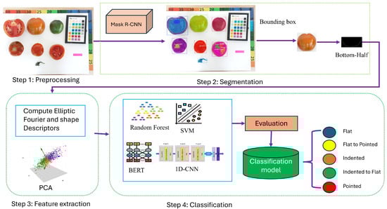
Figure 1.
Illustration of the proposed framework for tomato shape classification.
2.1. Extracting Tomato Object Using Mask-Rcnn
Mask R-CNN was introduced in 2018 by He, Kaiming, et al. [27]. They added a parallel branch to the existing Faster R-CNN to deal with instance segmentation. Mask R-CNN was developed to detect objects and mask objects from images. It has been used in different studies over the few years: Anantharaman et al. utilized Mask R-CNN on oral pathology [28], they focused on two common diseases and achieved the segmentation of those sores from images of the oral cavity. By adding an edge detection branch and PAFPN to the Mask R-CNN model, Xu et al. [29] successfully implemented higher accuracy detection and segmention on tunnel leakage and spalling regradless of the complicated background of surfaces.
In this study, tomato images were captured under conditions that included background elements such as a color reference card and a ruler. To isolate the tomatoes from these extraneous objects, we applied Mask R-CNN to segment the fruits and construct a refined dataset specifically designed for tomato shape classification. Subsequently, we extracted tomato contours using thresholding and contour detection functions implemented in the OpenCV framework. As previously discussed, the upper portions of the fruits exhibited no substantial variation; therefore, each tomato was divided into three sections, and the bottom region was used as input for the end-shape classification models.
2.2. End-Shape Classification Techniques
After isolating the bottom regions of the tomato images, we extracted the contour data of the fruits. To quantitatively describe these contours, we computed the Elliptic Fourier Descriptors (EFD) using the PyEFD library. We then applied Principal Component Analysis (PCA) to reduce data dimensionality and retain the most informative shape features. Subsequently, we evaluated a range of classification approaches, encompassing both traditional machine learning algorithms, such as Support Vector Machines (SVM) and Random Forest, and deep learning architectures, including Convolutional Neural Networks (CNN) and Bidirectional Encoder Representations from Transformers (BERT).
2.2.1. Elliptic Fourier Descriptors (EFD)
Extracting Elliptic Fourier Descriptors (EFD) from images of animals and plants is a widely adopted approach in morphological and shape-based studies. This technique enables the quantitative characterization of object contours. For instance, Ishikawa et al. [3] employed the freeware SHAPE (v1.3) [30] to quantitatively analyze strawberry contour lines. In contrast, to establish a more flexible and customizable workflow, we utilized the PyEFD API (v1.6.0) rather than other software-based solutions.
Fourier descriptors have been extensively applied in research focused on the characterization of closed contours. The PyEFD package provides a Python implementation of the method proposed by Kuhl and Giardina [31], which approximates the contours of closed shapes using a Fourier series. Their approach derives Fourier coefficients from a chain-encoded contour, where the chain code defined by Freeman [32] represents the contour as a continuous piecewise linear function approximating the object’s boundary. The Fourier series expansion for the x and y projections of the chain code of the closed contour is shown below:
where t stands for time intervals and T stands for total contour length. The coefficients were:
In this study, we used the function from the imported package to extract the Fourier coefficients , which represent the shape features. These coefficients are normalized by default, making them invariant to rotation and scale.
2.2.2. Principal Components Analysis (PCA)
When working with high dimensional datasets, it can be challenging to identify the most essential features. Processing all available data may be time-consuming and inefficient, as not every variable is critical to the research. Principal components analysis (PCA) [33] addresses this issue by eliminating redundant information and revealing underlying patterns within the dataset.
PCA is an unsupervised method that enables us to select the most critical attributes of the data set, thus reducing the dimensions. It is derived from the orthogonal linear transformation technique, which projects the attributes of a data set onto a new coordinate system. By doing so, we can obtain the facts that describe the most variance, which are the principal components. The method we used was provided by scikit-learn library [34]. The parameter in the function can be set in two ways: If 0 < < 1, the PCA returns the number of components such that the amount of variance that needs to be explained is greater than the percentage . On the other hand, we can also set directly to our desired lower dimension.
2.2.3. Traditional Machine Learning and Deep Learning Model for Tomato Shape Classification
To evaluate the performance of tomato shape prediction, several traditional machine learning and deep learning models were implemented and compared. These include Random Forest (RF), Support Vector Machine (SVC), 1D Convolutional Neural Networks (1D-CNNs), and Bidirectional Encoder Representations from Transformers (BERT).
Support vector machines (SVMs) are a collection of supervised learning methods used for classification, regression, and outlier detection. The purpose of SVM is to discover a hyperplane in an N-dimensional space that accurately categorizes the data points into distinct classes. To classify the data points with more confidence, we need to find a hyperplane that provides maximum margin. In this study, we tried the common LinearSVC and also the SVC with the polynomial kernel to improve precision. Both employed algorithm was provided by skicit-learn [34].
Random forest (RF) is a supervised learning algorithm. It is a kind of ensemble method that combines multiple models to achieve a better result. RF consists of several decision trees of different samples of the dataset, then it takes the maximum voting for classification or averages of predictions for regression. The algorithm we used was provided by skicit-learn [34].
1D-CNN has often been adopted in image classification and recognition. In Sharma et al.’s work [8], they tried the CNN method with four layers (an input layer, a convolutional layer, a ReLU activation layer, and a Batch Normalisation layer) to classify carrots by shape. We were inspired to structure a 1D-CNN network for categorizing tomatoes by their end shapes. The Elliptic Fourier Descriptor (EFD) coefficients extracted from each tomato contour were used as input features for the 1D-CNN model. Ten harmonics were computed for each contour, and the resulting coefficients were concatenated and flattened into a one-dimensional sequence. Each flattened EFD vector was reshaped into a 1D array corresponding to the sequence length of the coefficients. This representation enables the Conv1D layers to treat the ordered Fourier coefficients as sequential features, allowing the network to learn both local and global dependencies along the harmonic sequence. The proposed model comprises three convolutional blocks with 64 filters each, followed by batch normalization and ReLU activation. After the third convolutional layer, a global average pooling (GAP) layer was applied, followed by a fully connected layer with 32 units, ReLU activation, and a dropout rate of 0.5 to prevent overfitting. Finally, a softmax output layer was used, with the number of units corresponding to the number of tomato shape classes. We also applied early stopping and the save-best-only strategy to prevent overfitting and enhance model generalization.
BERT is a self-attention language representation model built by Google [35]. It is a pre-trained model that conditions on both sides of the unlabeled context. With fine-tuning by adding one additional layer, BERT can be exploited in tasks such as classification, question answering, next sentence prediction, and more. Although BERT was originally developed for natural language processing tasks, recent studies have demonstrated its adaptability for modeling structured numeric sequences by treating numerical feature vectors as sequential embeddings [36,37,38]. In this study, the Elliptic Fourier Descriptor (EFD) coefficients representing tomato contours were organized as ordered numeric sequences and normalized to form a one-dimensional input analogous to token embeddings in language models. These sequences were then processed using a modified BERT architecture to capture long-range dependencies among Fourier coefficients through self-attention mechanisms. This adaptation enables the model to learn complex relationships between different frequency components of the shape. There are two kinds of BERT models. One is the BERT , which consists of 12 layers of Transformer encoder, 12 attention heads, 768 hidden sizes, and 110M parameters. Another is the BERT , which comprises 24 layers of Transformer encoder,16 attention heads, 1024 hidden size, and 340 parameters. Though the larger model performs better, exploiting it requires more power and effort. Thus, we use the one in our study. In our BERT classification structure, we first tokenized our input data using the function . The model then produces an embedding vector of size 768 for each token, which we will later use as an input for our classifier. Then we add a layer of a ReLU activation; after that, we can start the PyTorch (v2.2) training loop. Our model consists of 10 epochs. Since we are dealing with multi-class classification, we use Categorical Cross-Entropy as our loss function.
2.3. Performance Measures
2.3.1. Performance Metrics for Segmentation Models
To assess the performance of our image segmentation models, we employed the evaluation metric: Intersection over Union (IoU).
Intersection over Union
The IoU metric, also known as the Jaccard Index, is widely used to measure the accuracy of image segmentation models. It is defined as the ratio between the area of overlap (intersection) and the area encompassed by both the predicted segmentation and the ground truth (union). The IoU metric is formulated as follows:
where denotes the for class c; (true positive) is the number of pixels correctly classified as class c; (false positive) is the number of pixels incorrectly classified as class c; and (false negative) is the number of pixels belonging to class c but not predicted as such.
2.3.2. Performance Metrics for Shape Classification Models
To evaluate the performance of our classification model, we employed the following four metrics:
The overall accuracy of our classifier derives from the correctness of the predictions. Between 0 and 1, the higher the accuracy grows, the better our classifier is functioning. By comparing the accuracy of the models we built from different methods, we can observe the performance of each model.
Considering the confusion matrix above, we can reach the accuracy formula:
The precision indicates the ratio of correctly predicted categories from all predicted categories. It is a within-class classification metric that explains how precise the models are in determining the correct classes for the tomatoes. Precision is calculated by the following formula:
Recall reveals how good the model is at accurately predicting all the positive observations from the given images. While the precision metric penalizes errors on , the recall metric penalizes errors on . It is calculated by the following formula:
The score is the harmonic mean of recall and precision, it seeks a balance between false negatives and false positives. score ranges between 0 and 1, the higher we get, the better precision and recall we hold. On the other hand, if , it means either the precision or the recall was zero. We can attain the F1 score by the
3. Experiment and Results
3.1. Data Collection and Processing
The dataset used in this study was provided by our partner, KNOW-YOU Seed Co. in Pingtung, Taiwan. Based on manual sorting conducted by their experienced fruit growers, five distinct tomato classes were identified, as illustrated in Figure 2. Tomato shapes were classified into five categories: “Flat”, characterized by an elliptical bottom; “Flat to Pointed”, with a slight protrusion from the standard curve; “Indented”, where the contour curves inward toward the fruit’s center; “Indented to Flat”, similar to the “indented” type but with smoother boundaries; and “Pointed”, exhibiting a more pronounced bulge than the “Flat to Pointed” class. In Figure 2, the left side of each category displays the original tomato image, while the right side presents the extracted contour of the bottom half. As illustrated in Figure 2, these shape categories are difficult to distinguish due to their subtle morphological differences.
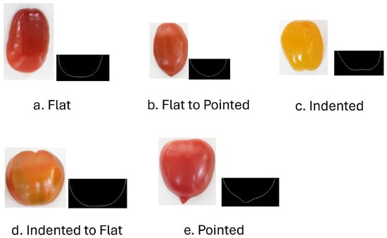
Figure 2.
Example of tomato images from distinct types of shape.
Table 1 summarizes the number of samples for each shape type in the training and testing sets. The dataset was randomly shuffled and split, with 80% (606 samples) allocated for training and 20% (151 samples) for testing. The images were pre-processed using Mask R-CNN in combination with the OpenCV framework. Shape data were obtained by extracting objects from the images, delineating the fruit contours, and cropping out the upper half of each fruit. The remaining bottom half was used as the dataset for tomato shape classification.

Table 1.
The statistical information for the tomato shape classification dataset.
Next, the contour images were converted to binary form to facilitate subsequent transformations, using the OpenCV binary thresholding function. In this process, pixels with intensities greater than a specified threshold were assigned a value of 255 (white), while the rest were set to 0 (black). The image data were not converted directly into pixel values, as this could produce unstable tomato contours; given the importance of boundary precision in this study, such an approach was avoided. After converting the contour data into numerical arrays, the function from the PyEFD module was applied to extract the coefficients of the elliptic Fourier descriptors representing the shapes.
3.2. Experimental Setup
The 1D Convolutional Neural Network (1D-CNN) and BERT models were trained for 500 epochs using the Adam optimizer with a batch size of 8. To enhance training stability and retain the best-performing models, two Keras callbacks were employed: ReduceLROnPlateau and ModelCheckpoint. The ReduceLROnPlateau callback dynamically adjusted the learning rate based on validation loss, reducing it by a factor of 0.5 if no improvement was observed for 20 consecutive epochs, with an initial learning rate of 0.001 and a minimum threshold of 0.0001. The ModelCheckpoint callback was used to save the model weights corresponding to the best validation performance.
For the Random Forest classifier, the number of estimators was set to 100, while other hyperparameters remained at their default values. The SVM model was configured with a polynomial kernel and a regularization parameter of C = 5, which was identified as optimal during preliminary experiments.
To investigate the effect of dimensionality reduction on classification performance, an additional set of experiments incorporated Principal Component Analysis (PCA). The number of components was determined by retaining 99% of the variance ( = 0.99). Furthermore, extensive data augmentation techniques, including flipping, rotation, scaling, and random cropping, were applied to improve model generalization.
For traditional machine learning models like Random Forest and SVM, we use 5-fold cross-validation, which splits the training data into five parts and rotates each as a validation set to estimate model performance, since these models train quickly and do not require iterative optimization. In contrast, for deep learning models like BERT and 1D CNN, we reserve 10% of the training data as a validation set in every epoch, because training these models is computationally expensive and iterative, requiring ongoing validation to monitor overfitting, guide early stopping, and adjust hyperparameters.
Finally, all the models were implemented and trained using Keras 2.4.3 (developed by Google, Mountain View, CA, USA). All experiments were carried out on a server with an Intel Core i7-12700 CPU and 62 GB of RAM, and an NVIDIA GeForce RTX 4090 GPU.
3.3. Application of Mask R-CNN to Raw Images
The model was employed to perform instance segmentation on raw images to construct the tomato dataset for training. Specifically, fourteen classes, namely background (BG), core, section, in, vertical surface, immature tomato, blossom, sepal, ruler, bottom, up, stem scar, cross, locules inside, and seed cavity, were segmented from the raw images. Each segmented class was used for further processing to characterize tomato features. However, the present work focuses solely on determining tomato shape; therefore, only the “vertical surface” class was considered. The classification accuracy results are presented in Table 2. Furthermore, the bounding box of the tomato’s vertical surface was cropped to prepare the dataset for tomato shape classification. To prepare the labeled data for the Mask R-CNN segmentation model, the tomato dataset was manually annotated using the VGG Image Annotator [39]. The segmentation model was trained on the training set through transfer learning from a pre-trained ImageNet model. During training, 10% of the training data was randomly allocated as a validation set for model evaluation and fine-tuning. The Mask R-CNN achieved an accuracy of 91.06% for the entire fruit class.
Table 2.
Result of Mask R-CNN model.
Figure 3 illustrates the output of the Mask R-CNN model, which generates predictions for multiple input images and extracts the “vertical surface” class from each image. Ultimately, this process yields a set of tomatoes for the shape classification stage.
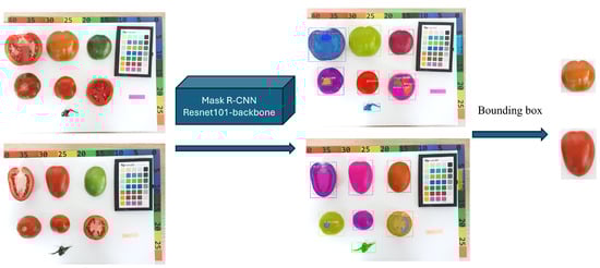
Figure 3.
Illustration of extracting tomato object using mask-rcnn.
3.4. Evaluating the Performance of Different Models for Tomato Shape Classification
To determine the most effective method for classifying tomato end shape contours, we evaluated traditional machine learning algorithms, including Random Forest and Support Vector Machine, along with deep learning models such as 1D-CNN and BERT, to assess their performance on fruit contour data. The performance of each model is summarized in Table 3. Among the traditional machine learning methods, the Random Forest classifier outperformed the Support Vector Machine on the original dataset. In contrast, 1D-CNN and BERT achieved relatively lower accuracy compared to the traditional approaches. The highest accuracy, 79.4%, was obtained by the Random Forest model. The Random Forest model achieved the highest accuracy because the task involved compact, well-engineered contour features and a relatively small dataset, where Random Forest’s ability to handle structured numerical data and avoid overfitting gave it an advantage over data-hungry deep learning models like 1D-CNN and BERT. The standard deviation values reported for SVM (4.04%) and Random Forest (4.03%) indicate moderate variability in model performance across the K-fold cross-validation splits. Given that Random Forest achieves the highest mean accuracy (79.4%), the standard deviation(SD) suggests that while the model performs consistently on average, its performance can fluctuate slightly depending on the specific training and validation folds. This variability is expected for datasets of limited size, where small changes in the training subset can impact the model’s predictions. For deep learning models like 1D-CNN and BERT, standard deviation is not reported because a fixed 10% validation set was used during each epoch rather than K-fold cross-validation. Consequently, while the deep learning models provide mean accuracy values, their variability across runs is not directly quantified in this table. Overall, the relatively low SD for Random Forest demonstrates both strong performance and reasonable stability, reinforcing its suitability as the best-performing model for tomato shape classification in this study.
Table 3.
Classification result of tomato shape using different models.
To statistically evaluate the differences in model performance, we conducted pairwise McNemar’s tests on the predictions of SVM, Random Forest, 1D CNN, and BERT as shown in Table 4. The results indicate that Random Forest performs significantly better than SVM, 1D CNN, and BERT. SVM is significantly better than 1D CNN, but its difference with BERT is not statistically significant. Finally, there is no significant difference between 1D CNN and BERT. These results confirm that the observed differences in accuracy among the models are meaningful and not due to random chance.
Table 4.
Pairwise McNemar’s test results for all models. “First Only” and “Second Only” indicate the number of samples where only the first or second model, respectively, made a correct prediction.
3.5. Further Investigate Using PCA
Principal Component Analysis (PCA) is a widely used dimensionality reduction technique that transforms high-dimensional data into a smaller set of uncorrelated variables while preserving most of the original variance. Applying PCA before classification can help remove noise, reduce computational complexity, and highlight the most informative features. In this section, we investigate the impact of PCA on model performance for tomato end shape contour classification. By projecting the original contour feature set into a lower-dimensional space, we aim to assess whether PCA can enhance classification accuracy or improve model efficiency across both traditional machine learning algorithms and deep learning models. Figure 4 compares the results between the original data using EFD and the reduced data after applying PCA. As shown in Figure 4, in most cases, classifiers trained on data processed with Principal Component Analysis (orange bars) achieved higher testing accuracy in our study. The only exception is the Random Forest classifier, which performed better on the original Elliptic Fourier Descriptor features than on the PCA-reduced features. PCA helped most models, such as SVM, 1D-CNN, and BERT, focus on the most discriminative features by reducing redundancy and noise in the contour data, thereby improving generalization and making the classification task easier. However, Random Forest already excels at handling high-dimensional, correlated data through its inherent feature selection, which identifies and uses only the most relevant features for each split. As a result, PCA’s transformation removed some useful shape information, slightly lowering the Random Forest’s performance.
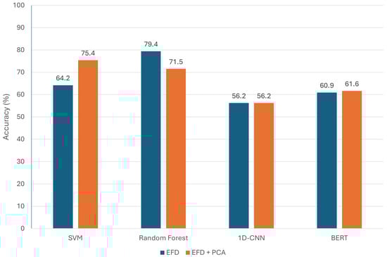
Figure 4.
Accuracy comparison of classification models with and without PCA.
3.6. Discussion
Figure 5 and Figure 6 illustrate class separability before and after model training with our best model, the Random Forest, respectively. We observed that the PCA of the original feature space (Figure 5) shows overlapping clusters, whereas the PCA of the Random Forest output probabilities (Figure 6) demonstrates well-separated clusters. This indicates the Random Forest model successfully learned to classify the tomato shape features.
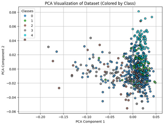
Figure 5.
An illustration of class separability in the original feature space prior to model training.
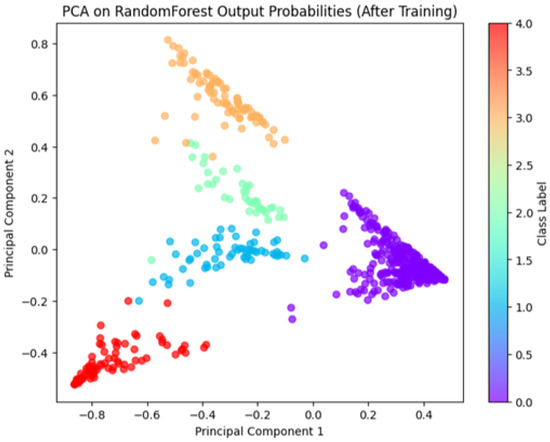
Figure 6.
An illustration of the PCA of Random Forest output probabilities for our dataset.
Table 5 displays other evaluation metrics result for each class using Random Forest model. Overall, the model achieved strong performance for the majority of classes, with particularly high precision for “flat” (95%) and balanced precision and recall for “pointed” (86%). These outcomes indicate that the model was effective in distinguishing tomatoes with distinct shape characteristics.
Table 5.
Classification report of the Random Forest model for tomato shape categories.
For the “indented” class, the model achieved a recall of 88% and an F1-score of 78% despite the relatively small sample size, suggesting that the contour-based features captured discriminative information for this category. By contrast, transitional classes such as “flat to pointed” and “indented to flat” yielded lower performance, with F1-scores of 22% and 59%, respectively. The low precision for “flat to pointed” 14% highlights the difficulty of distinguishing this class, likely due to both the limited number of samples and the morphological overlap between the “flat” and “pointed” classes. Similarly, “indented to flat” showed reasonable recall 77% but lower precision (48%), reflecting a tendency of the model to over-predict this transitional shape.
Table 6 presents confusion matrix for tomato shape classification using Random Forest model. From the confusion matrix, it can be observed that most misclassifications occurred in the transitional classes, particularly “Flat to Pointed” and “Indented to Flat”, which were frequently predicted as “Flat”. This suggests that the model tends to be biased toward the dominant “Flat” class when the shape characteristics are intermediate or less distinct. Such misclassification likely arises from the overlapping morphological traits between adjacent categories, where contour differences are subtle and difficult to distinguish based solely on shape descriptors. In contrast, the “Pointed” and “Indented” classes were classified with relatively higher accuracy, indicating that more distinct contour features contribute to better separability. These results highlight the challenge of accurately classifying transitional tomato shapes and suggest that integrating complementary features such as color or texture information could improve performance in future work.
Table 6.
Confusion matrix for tomato shape classification. Rows represent true labels, and columns represent predicted labels.
Furthermore, we visualized examples of misclassified images where tomatoes from the “Indented to Flat” and “Flat to Pointed” classes were incorrectly predicted as “Flat” in Figure 7. These errors primarily arise from the subtle differences in contour curvature and the smooth transition between shape categories. As shown in Figure 7a, tomatoes in the “Indented to Flat” class often exhibit only shallow indentations, making their outlines visually similar to “Flat” samples, especially under varying lighting or viewing angles. Similarly, Figure 7b shows “Flat to Pointed” tomatoes with slight tapering that may not be distinct enough for the model to capture through shape descriptors alone. This indicates that transitional classes pose a greater challenge for classification, suggesting that integrating complementary features such as texture or color information could help improve model robustness and discrimination between closely related shape categories.
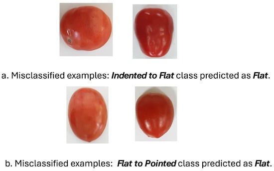
Figure 7.
Illustration of misclassification cases from the Indented to Flat class incorrectly predicted as Flat.
Analysis of the confusion matrix and misclassified samples revealed that most errors occurred among tomato varieties with highly similar contour shapes, where subtle differences in curvature or aspect ratio caused class confusion. In addition, noise and irregularities from image acquisition, such as partial occlusion, uneven lighting, or minor segmentation errors, sometimes distorted the extracted Elliptic Fourier Descriptors (EFDs). These results suggest that while the proposed model effectively captures global shape characteristics, it remains sensitive to fine-grained contour variations and data inconsistencies. Future work will focus on expanding the dataset and refining the model architecture to improve robustness against contour noise and intra-class similarity.
4. Conclusions
This study presents a shape-based workflow for tomato classification using Mask R-CNN segmentation and Elliptic Fourier Descriptors (EFDs). Random Forest achieved the highest accuracy (79.4%) among the evaluated models, demonstrating robust classification across distinct shape categories. Transitional classes remain challenging due to class overlap and imbalance. These findings highlight the practical value of contour-based shape analysis as a complement to traditional color-based approaches. Future work will focus on integrating shape and color features, enhancing feature representations, and addressing class imbalance to further improve accuracy and generalization in real-world agricultural applications.
Author Contributions
All authors contributed to the study conception and design. The supervision of revision and experiments were performed by T.-T.H., R.M.I.K. and H.Y.W.; Material preparation, data collection and analysis were performed by T.-T.H.; The draft of the manuscript was written by H.Y.W. and V.L.H. and all authors commented on previous versions of the manuscript. All authors have read and agreed to the published version of the manuscript.
Funding
This work was supported by the National Science and Technology Council of Taiwan (Grant No NSTC 114-2313-B-032-001).
Data Availability Statement
The datasets generated and/or analysed during the current study are available from the corresponding author on reasonable request.
Conflicts of Interest
Author Rosdyana Mangir Irawan Kusuma was employed by the company ASUSTeK Computer Inc. The remaining authors declare that the research was conducted in the absence of any commercial or financial relationships that could be construed as a potential conflict of interest.
References
- Barten, J.H.M.; Scott, J.W.; Gardner, R.G. Characterization of blossom-end morphology genes in tomato and their usefulness in breeding for smooth blossom-end scars. J. Am. Soc. Hortic. Sci. 1994, 119, 798–803. [Google Scholar] [CrossRef]
- Hossain, M.S.; Al-Hammadi, M.; Muhammad, G. Automatic fruit classification using deep learning for industrial applications. IEEE Trans. Ind. Inform. 2018, 15, 1027–1034. [Google Scholar] [CrossRef]
- Ishikawa, T.; Hayashi, A.; Nagamatsu, S.; Kyutoku, Y.; Dan, I.; Wada, T.; Oku, K.; Saeki, Y.; Uto, T.; Tanabata, T.; et al. Classification of strawberry fruit shape by machine learning. Int. Arch. Photogramm. Remote Sens. Spat. Inf. Sci. 2018, 42, 463–470. [Google Scholar] [CrossRef]
- Brewer, M.T.; Lang, L.; Fujimura, K.; Dujmovic, N.; Gray, S.; van der Knaap, E. Development of a controlled vocabulary and software application to analyze fruit shape variation in tomato and other plant species. Plant Physiol. 2006, 141, 15–25. [Google Scholar] [CrossRef]
- Gonzalo, M.J.; Brewer, M.T.; Anderson, C.; Sullivan, D.; Gray, S.; van der Knaap, E. Tomato fruit shape analysis using morphometric and morphology attributes implemented in Tomato Analyzer software program. J. Am. Soc. Hortic. Sci. 2009, 134, 77–87. [Google Scholar] [CrossRef]
- Rodríguez, G.R.; Moyseenko, J.B.; Robbins, M.D.; Morejón, N.H.; Francis, D.M.; van der Knaap, E. Tomato Analyzer: A useful software application to collect accurate and detailed morphological and colorimetric data from two-dimensional objects. JoVE J. Vis. Exp. 2010, 37, e1856. [Google Scholar]
- Visa, S.; Cao, C.; Gardener, B.M.; van der Knaap, E. Modeling of tomato fruits into nine shape categories using elliptic fourier shape modeling and Bayesian classification of contour morphometric data. Euphytica 2014, 200, 429–439. [Google Scholar] [CrossRef]
- Sharma, R.; Agarwal, A.; Mamatha, H.R. Classification of carrots based on shape analysis using machine learning techniques. In Proceedings of the 2021 Third International Conference on Intelligent Communication Technologies and Virtual Mobile Networks (ICICV), Tirunelveli, India, 4–6 February 2021; IEEE: Piscataway, NJ, USA, 2021. [Google Scholar]
- Masuda, T. Leaf area estimation by semantic segmentation of point cloud of tomato plants. In Proceedings of the IEEE/CVF International Conference on Computer Vision, Montreal, QC, Canada, 10–17 October 2021; pp. 1381–1389. [Google Scholar]
- Bargoti, S.; Underwood, J.P. Image segmentation for fruit detection and yield estimation in apple orchards. J. Field Robot. 2017, 34, 1039–1060. [Google Scholar] [CrossRef]
- Kang, H.; Chen, C. Fruit detection and segmentation for apple harvesting using visual sensor in orchards. Sensors 2019, 19, 4599. [Google Scholar] [CrossRef] [PubMed]
- Kang, H.; Chen, C. Fruit detection, segmentation and 3d visualisation of environments in apple orchards. Comput. Electron. Agric. 2020, 171, 105302. [Google Scholar] [CrossRef]
- Mostafa, A.M.; Kumar, S.A.; Meraj, T.; Rauf, H.T.; Alnuaim, A.A.; Alkhayyal, M.A. Guava disease detection using deep convolutional neural networks: A case study of guava plants. Appl. Sci. 2021, 12, 239. [Google Scholar] [CrossRef]
- Mureşan, H.; Oltean, M. Fruit recognition from images using deep learning. arXiv 2017, arXiv:1712.00580. [Google Scholar] [CrossRef]
- Shahi, T.B.; Sitaula, C.; Neupane, A.; Guo, W. Fruit classification using attention-based mobilenetv2 for industrial applications. PLoS ONE 2022, 17, 0264586. [Google Scholar] [CrossRef]
- Sun, K.; Wang, X.; Liu, S.; Liu, C. Apple, peach, and pear flower detection using semantic segmentation network and shape constraint level set. Comput. Electron. Agric. 2021, 185, 106150. [Google Scholar] [CrossRef]
- Ganesh, P.; Volle, K.; Burks, T.; Mehta, S. Deep orange: Mask R-CNN based orange detection and segmentation. IFAC-PapersOnLine 2019, 52, 70–75. [Google Scholar] [CrossRef]
- Xiong, L.; Wang, Z.; Liao, H.; Kang, X.; Yang, C. Overlapping citrus segmentation and reconstruction based on mask R-CNN model and concave region simplification and distance analysis. J. Phys. Conf. Ser. 2019, 1345, 032064. [Google Scholar]
- Yu, Y.; Zhang, K.; Yang, L.; Zhang, D. Fruit detection for strawberry harvesting robot in non-structural environment based on Mask-RCNN. Comput. Electron. Agric. 2019, 163, 104846. [Google Scholar] [CrossRef]
- Liu, X.; Zhao, D.; Jia, W.; Ji, W.; Ruan, C.; Sun, Y. Cucumber fruits detection in greenhouses based on instance segmentation. IEEE Access 2019, 7, 139635–139642. [Google Scholar] [CrossRef]
- Afonso, M.; Fonteijn, H.; Fiorentin, F.S.; Lensink, D.; Mooij, M.; Faber, N.; Polder, G.; Wehrens, R. Tomato fruit detection and counting in greenhouses using deep learning. Front. Plant Sci. 2020, 11, 571299. [Google Scholar] [CrossRef]
- Jia, W.; Tian, Y.; Luo, R.; Zhang, Z.; Lian, J.; Zheng, Y. Detection and segmentation of overlapped fruits based on optimized mask R-CNN application in apple harvesting robot. Comput. Electron. Agric. 2020, 172, 105380. [Google Scholar] [CrossRef]
- Ni, X.; Li, C.; Jiang, H.; Takeda, F. Deep learning image segmentation and extraction of blueberry fruit traits associated with harvestability and yield. Hortic. Res. 2020, 7, 110. [Google Scholar] [CrossRef]
- Lin, G.; Tang, Y.; Zou, X.; Wang, C. Three-dimensional reconstruction of guava fruits and branches using instance segmentation and geometry analysis. Comput. Electron. Agric. 2021, 184, 106107. [Google Scholar] [CrossRef]
- Chu, P.; Li, Z.; Lammers, K.; Lu, R.; Liu, X. Deep learning-based apple detection using a suppression mask R-CNN. Pattern Recogn. Lett. 2021, 147, 206–211. [Google Scholar] [CrossRef]
- Tran, K.-D.; Ho, T.-T.; Huang, Y.; Le, N.Q.K.; Tuan, L.Q.; Ho, V.L. MASPP and MWASP: Multi-head self-attention based modules for UNet network in melon spot segmentation. J. Food Meas. Charact. 2024, 18, 3935–3949. [Google Scholar] [CrossRef]
- He, K.; Gkioxari, G.; Dollár, P.; Girshick, R. Mask r-cnn. In Proceedings of the IEEE International Conference on Computer Vision, Venice, Italy, 22–29 October 2017. [Google Scholar]
- Anantharaman, R.; Velazquez, M.; Lee, Y. Utilizing mask R-CNN for detection and segmentation of oral diseases. In Proceedings of the 2018 IEEE International Conference on Bioinformatics and Biomedicine (BIBM), Madrid, Spain, 3–6 December 2018; IEEE: Piscataway, NJ, USA, 2018. [Google Scholar]
- Xu, Y.; Li, D.; Xie, Q.; Wu, Q.; Wang, J. Automatic defect detection and segmentation of tunnel surface using modified Mask R-CNN. Measurement 2021, 178, 109316. [Google Scholar] [CrossRef]
- Iwata, H.; Ukai, Y. SHAPE: A computer program package for quantitative evaluation of biological shapes based on elliptic Fourier descriptors. J. Hered. 2002, 93, 384–385. [Google Scholar] [CrossRef]
- Kuhl, F.P.; Giardina, C.R. Elliptic Fourier features of a closed contour. Comput. Graph. Image Process. 1982, 18, 236–258. [Google Scholar] [CrossRef]
- Freeman, H. Computer processing of line-drawing images. ACM Comput. Surv. CSUR 1974, 6, 57–97. [Google Scholar] [CrossRef]
- Clark, N.R.; Ma’ayan, A. Introduction to statistical methods to analyze large data sets: Principal components analysis. Sci. Signal. 2011, 4, tr3. [Google Scholar] [CrossRef]
- Pedregosa, F.; Varoquaux, G.; Gramfort, A.; Michel, V.; Thirion, B.; Grisel, O.; Blondel, M.; Prettenhofer, P.; Weiss, R.; Dubourg, V.; et al. Scikit-learn: Machine learning in Python. J. Mach. Learn. Res. 2011, 12, 2825–2830. [Google Scholar]
- Devlin, J.; Chang, M.-W.; Lee, K.; Toutanova, K. Bert: Pre-training of deep bidirectional transformers for language understanding. arXiv 2018, arXiv:1810.04805. [Google Scholar]
- Padhi, I.; Schiff, Y.; Melnyk, I.; Rigotti, M.; Mroueh, Y.; Dognin, P.; Ross, J.; Nair, R.; Altman, E. Tabular transformers for modeling multivariate time series. In Proceedings of the ICASSP 2021—2021 IEEE International Conference on Acoustics, Speech and Signal Processing (ICASSP), Toronto, ON, Canada, 6–11 June 2021; IEEE: Piscataway, NJ, USA, 2021; pp. 3565–3569. [Google Scholar]
- Badaro, G.; Saeed, M.; Papotti, P. Transformers for tabular data representation: A survey of models and applications. Trans. Assoc. Comput. Linguist. 2023, 11, 227–249. [Google Scholar] [CrossRef]
- Luetto, S.; Garuti, F.; Sangineto, E.; Forni, L.; Cucchiara, R. One transformer for all time series: Representing and training with time-dependent heterogeneous tabular data. Mach. Learn. 2025, 114, 145. [Google Scholar] [CrossRef]
- Abhishek Dutta, Visual Geometry Group, Oxford University. VGG Image Annotator: An Image Annotation Tool That Can Be Used to Define Regions in an Image and Create Textual Descriptions of Those Regions. Software 2016. Available online: https://annotate.officialstatistics.org/ (accessed on 1 January 2025).
Disclaimer/Publisher’s Note: The statements, opinions and data contained in all publications are solely those of the individual author(s) and contributor(s) and not of MDPI and/or the editor(s). MDPI and/or the editor(s) disclaim responsibility for any injury to people or property resulting from any ideas, methods, instructions or products referred to in the content. |
© 2025 by the authors. Licensee MDPI, Basel, Switzerland. This article is an open access article distributed under the terms and conditions of the Creative Commons Attribution (CC BY) license (https://creativecommons.org/licenses/by/4.0/).