A Performance Comparison of CNN Models for Bean Phenology Classification Using Transfer Learning Techniques

Abstract

The early and precise identification of the different phenological stages of the bean (Phaseolus vulgaris L.) allows for the determination of critical and timely moments for the implementation of certain agricultural activities that contribute in a significant manner to the output and quality of the harvest, as well as the necessary actions to prevent and control possible damage caused by plagues and diseases. Overall, the standard procedure for phenological identification is conducted by the farmer. This can lead to the possibility of overlooking important findings during the phenological development of the plant, which could result in the appearance of plagues and diseases. In recent years, deep learning (DL) methods have been used to analyze crop behavior and minimize risk in agricultural decision making. One of the most used DL methods in image processing is the convolutional neural network (CNN) due to its high capacity for learning relevant features and recognizing objects in images. In this article, a transfer learning approach and a data augmentation method were applied. A station equipped with RGB cameras was used to gather data from images during the complete phenological cycle of the bean. The information gathered was used to create a set of data to evaluate the performance of each of the four proposed network models: AlexNet, VGG19, SqueezeNet, and GoogleNet. The metrics used were accuracy, precision, sensitivity, specificity, and F1-Score. The results of the best architecture obtained in the validation were those of GoogleNet, which obtained 96.71% accuracy, 96.81% precision, 95.77% sensitivity, 98.73% specificity, and 96.25% F1-Score.

1. Introduction

According to the Food and Agriculture Organization of the United Nations (FAO), plant plagues are among the main causes of the loss of over 40 percent of food crops worldwide, exceeding losses of up to USD 220 billion each year [1]. In Mexico, bean production contributes MXN 5927 million to the annual income. However, in 2021, the registered loss was more than MXN 222 million, mainly due to diseases caused by viruses transmitted in seeds, aphids, white flies, and other similar insects [2]. Several factors interfere with food security, such as climate change [3,4,5], the lack of pollinators [6,7], plagues and plant diseases [8], the result of the COVID-19 pandemic, and the present war between Russia and Ukraine [9], among others.

Insect plagues, diseases, and other organisms significantly affect the quality and production of crops. These organisms feed off plants and transmit diseases that can cause severe disruption in the growth and development of plants, causing a major impact on food security, the economy, and the environment, thereby decreasing the availability of food, increasing production costs, and affecting the growth of rural areas and developing countries [10].

It is important to mention the strategies used to mitigate the effects produced by plagues and diseases around the world, such as the selection of resistant varieties, crop rotation, the use of natural enemies of plagues, and the rational use of chemical products, among others. More efforts need to be made to implement mechanisms and innovative strategies to reduce loss in food crops and sustainably contribute to food security [9,11,12].

In recent years, the use of artificial intelligence (AI) in applications has increased exponentially. Proof of this is the appearance of works related to image recognition, especially in the field of agriculture, where various approaches to using deep learning (DL) methods to classify the phenology of different food crops around the world have been presented. This allows us to have knowledge of the record of critical moments in the life cycle of the plant to program treatments, effectively and timely apply pesticides or fungicides, and prevent and control plagues and diseases; this offers great advantages in precision agriculture in a nonharmful manner, and it helps minimize damage to crops [13,14,15,16,17].

DL methods are used to identify the different phenological stages of crops, and there exists a diversity of approaches to address the classification of topics related to agricultural decision making that mainly influence the estimation of agricultural production. In this regard, the present work proposes a comparative study of the performance of four models of convolutional neural networks (CNNs), AlexNet, VGG19, SqueezeNet, and GoogleNet, in classifying the phenological stages of bean crops; the performance of each of the models is compared through the following metrics: accuracy, precision, sensitivity, specificity, and F-1 Score. The results are used to choose the architecture that best models the classification problem in bean phenology.

The goal of analyzing the different CNN architectures is to identify the best-performing one and, in the future, to embed networks in compact systems so that farmers can identify the phenological stages of plants, allowing them to take preventive measures.

The organization of the present work is structured as follows: Section 2 describes the most relevant works on transfer learning, related concepts, and a description of the CNN models used in the present work. Section 3 describes the methodology of the investigation work. Section 4 contains the obtained results and their discussion. Section 5 presents the conclusions, and finally, future work is described.

2. Related Work

DL has been used to obtain high-quality maps. In this regard, Ge et al. [18] mapped crops from different regions in the period from planting to vigorous growth and compared the maps obtained by using conventional methods with those obtained with DL, where the latter reached 87% accuracy.

On the other hand, Yang et al. [17] proposed the identification of the different phenological phases of rice from RGB images captured by a drone with a CNN model that incorporated techniques such as spatial pyramidal sampling, knowledge transfer, and external data, which are essential for timely estimation and output, in comparison to previous approaches where data on the vegetation index in temporal series and diverse methods based on thresholds were used. The obtained results show that the approach has high precision in the identification of the phenology of rice, with 83.9% precision and a mean absolute error (MAE) of 0.18.

The approach of learning by transfer is used in various applications, such as the prediction of the performance of numerous crops worldwide, where Wang et al. [19] used remote sensors with satellite images to estimate the outcome of soy crops through algorithms and deep learning, offering an inexpensive and efficient alternative in comparison to conventional techniques that are generally expensive and difficult to expand in regions with limited access to data.

Identifying the phenology in diverse crops allows for determining critical moments for timely agricultural activities. In this regard, Reeb et al. [20] implemented a pre-trained CNN model named ResNet18 to classify the phenology of A. petiolata, comparing the results obtained to the classification conducted by a group of non-expert humans. During the validation stage of the model, 86.4% of the results obtained from a set of 2448 images were classified correctly by the proposed model. Subsequently, an evaluation of the precision of the model was made and compared to human precision, where the model correctly classified 81.7% of a total of 241 images. In contrast, the non-expert humans achieved a precision of 78.6%.

On the other hand, Datt et al. [15] used the CNN to recognize eight phenological stages in apple crops. The knowledge transfer model used was Inception-v3, which trained a set of images from the Srinagar region in India. The number of images captured in the area was 1200, extending to 7000 images through data augmentation techniques, obtaining results in comparison to other models such as Xception, Xception-v3, ResNet50, VGG16, and VGG19 where the metric used was for F1-Score and achieved values of 0.97, 0.96, 0.66, 0.96, and 0.95, respectively.

Through the use of characteristic descriptors, Yalcin et al. [16] proposed the implementation of automatic learning algorithms to compare learning algorithms based on a CNN to recognize and classify phenological stages in various types of crops such as wheat, corn, barley, lentil, cotton, and pepper through images collected by cameras at farming stations located in parts of the territory of Turkey. The AlexNet model used for the classification of phenology significantly exceeded automatic learning algorithms during the performance evaluation.

The combination of conventional techniques with DL methods can offer alternatives to the solution of classification problems, such as the case of the application of hybrid methods, to get to know the estimation of agricultural production in the work carried out by Zhao et al. [21], in which they used the knowledge transfer technique to learn from an existing model based on the combination of biomass algorithms of wheat crops and the model of simple performance. The results show a precise estimation of the wheat harvest with both models since they reveal a good correlation of $R^2$ = 0.83 and a root mean squared error (RMSE) of 1.91 t ha⁻¹.

The use of temporal series and other techniques for phenological classification is usually relevant in the work carried out by Taylor et al. [22], who propose a model for creating temporal series of the phenological cycle. They use a hidden Markov post-process model to address the temporal correlation between images, reaching F1-Scores of 0.86 to 0.91. The results show the temporal progression of the crops from the emergency to the harvest, providing the daily phenological stages on a temporal scale.

DL techniques are used to classify the different phenological stages in different types of crops, including bean crops. The diversity of approaches and techniques used to classify images varies the obtained results compared to techniques and strategies used in diverse studies during the last decade. Thereupon, CNN produces trusted results, has a grand capacity for generalization in the classification of images, and has a high capacity for extracting features related to the phenology in different crops.

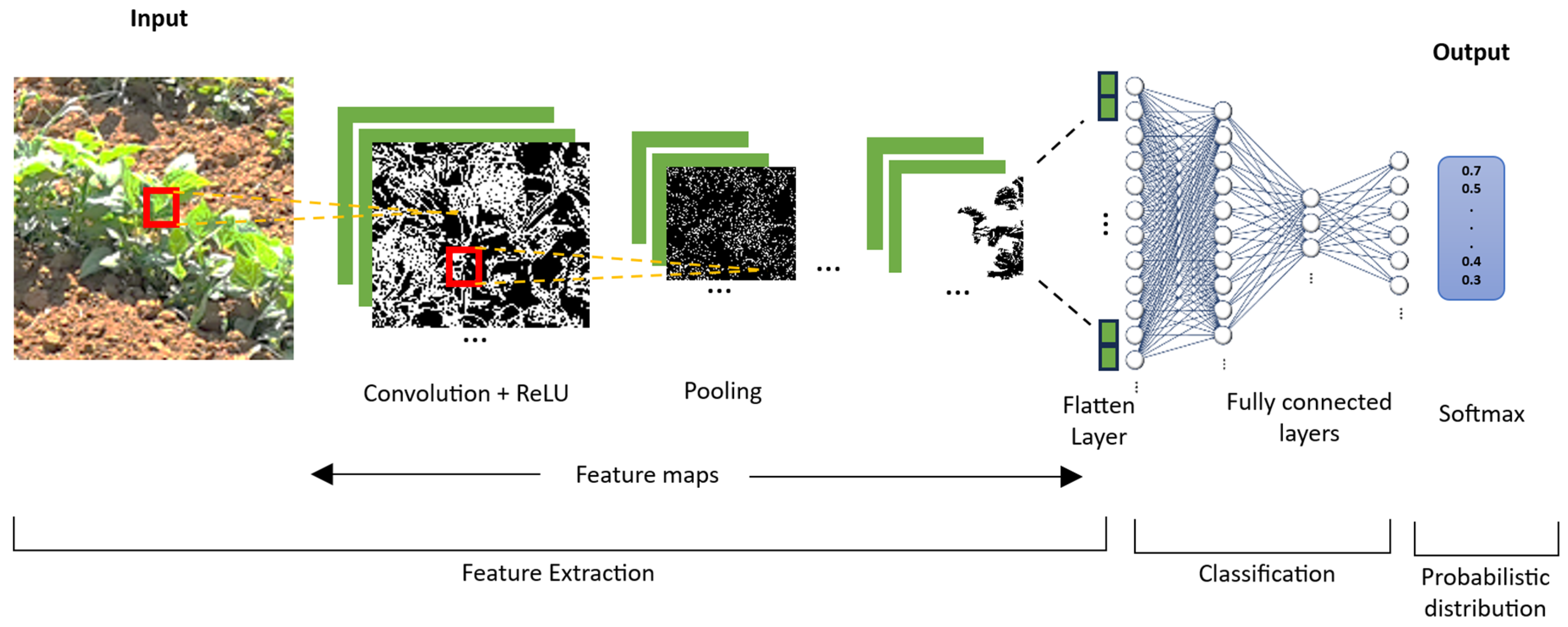
2.1. Convolutional Neural Networks (CNNs)

CNNs basically consist of three blocks: the first in a layer of convolution that allows the extraction of features of an image; the second is a block that consists of a layer of maximum grouping to execute a subsample of pixels and reduce the dimensionality, allowing the reduction of computational costs; and finally, the third block involves fully connected layers to provide the network with the capacity of classification [23,24,25]. The general description of the CNN architecture is shown in Figure 1, where features of the images are identified, extracted, and classified.

Figure 1. The architecture of convolutional network.

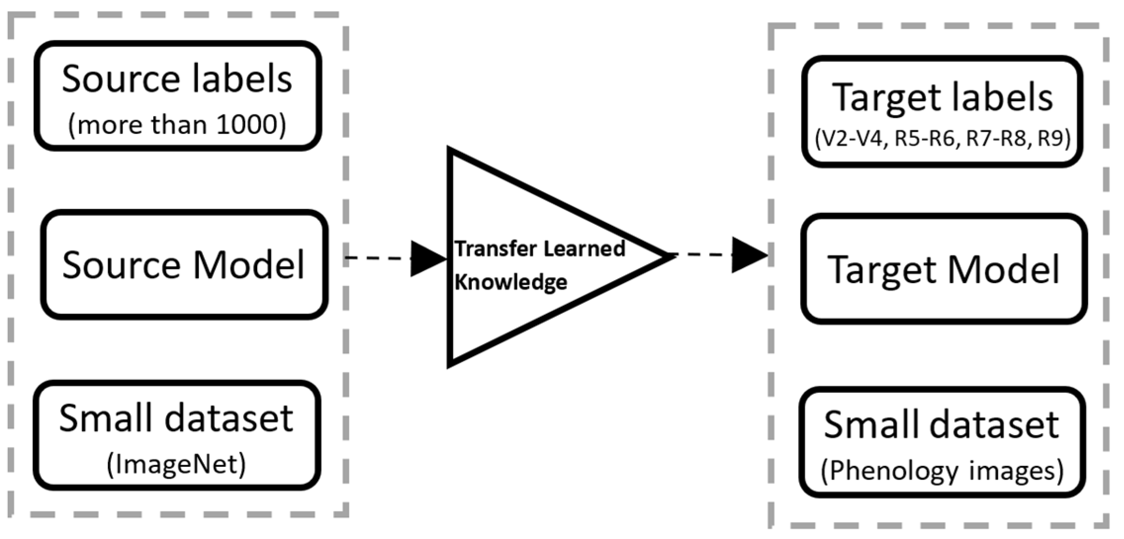
2.2. Transfer Learning

In general, CNN results are better if trained by more extensive data sets than small ones. However, many applications do not have large data sets, and transfer learning can be helpful in those applications where the data set is smaller in ImageNet [26]. For this reason, a re-trained model from large data sets can be used to learn new features from a comparatively smaller data set [27]. Figure 2 describes a block diagram of the transfer learning approach used in this study.

Figure 2. Block diagram of the concept of transfer learning.

Recently, the scientific community has taken a particular interest in the transfer learning approach in diverse fields, such as medicine and agriculture, among others [28,29,30,31]. This approach allows previously acquired knowledge and avoids training with large quantities of data when training new deep architecture models [28,32,33].

2.3. Re-Trained Neural Networks

Using a re-trained CNN model has significant advantages in comparison to the design of models from zero, which require large sets of data and training that can take considerable time, including weeks, translating into high computational costs. On the other hand, a re-trained model can have a high capacity for generalization and accelerate convergence [34].

In this study, four models of re-trained CNN were used to evaluate the performance in the image classification identifying phenological phases in bean crops: AlexNet, VGG19, SqueezeNet, and GoogleNet. A brief introduction of each of the re-trained models is included below.

2.3.1. AlexNet Model

The algorithms for object detection and image classification were evaluated with the AlexNet model developed by Krizhevsky et al. [35] and the ImageNet Large-Scale Visual Recognition Challenge (LSVRC) for the model training [36]. The architecture is characterized by using a new activating function, the Rectified Linear Unit (ReLU), to add non-linearity, solve the gradient evanescent problem, and accelerate network training. CNN consists of eight layers in total: the first five layers are of convolution, some of which are followed by max-pooling layers, and the following three layers are fully connected, followed by an exit layer of 1000 neurons for the SoftMax for multiclass classification. The AlexNet model was trained with over one million images from the ImageNet database created by Deng et al. [26]. The entry size of the images is 227 × 227, a total of 60 million parameters and 650 thousand neurons.

2.3.2. VGG19

The VGG19 network is a nineteen-layer deep convolutional neural network developed by Simonyan et al. [37]. This model uses small filters of 3 × 3 in each of the sixteen convolution layers. Next, it uses three fully connected layers to classify images into 1000 categories. The ImageNet database developed by Deng et al. [26] was used to train the VGG19 model. The layers used for the extraction of features are separated into five groups where a layer of max-pooling follows each group, and it is required to insert and image the size of 224 × 224 to generate the label corresponding to the exit.

2.3.3. SqueezeNet

The SqueezeNet architecture uses compression techniques to reduce the model size without compromising its performance with a fire module that, instead of using convolutional layers followed by grouping layers, uses a combination of filters that combine convolutions of 1 × 1 and 3 × 3 to reduce the number of parameters. The SqueezeNet model proposed by Iandola et al. [38] contains fifty times fewer parameters than the AlexNet model, has eighteen layers of profundity, and requires a size of 227 × 227.

2.3.4. GoogleNet

This model, also known as Inception v1, was developed by Szegedy et al. [32]. It consists of twenty-two layers of profundity with entry images the size of 224 × 224. GoogleNet uses average pooling after the last convolutional layer instead of fully connected layers. The convolution modules called “Inception modules” are composed of multiple convolutions of different sizes (1 × 1, 3 × 3, and 5 × 5), allowing the network to capture the features on different spatial layers, facilitating the representation of fine details and complex patterns.

Table 1 summarizes the main features in terms of the parameters used, profundity, and size of the different architectures of CNN networks proposed in this study.

Table 1. Summary of presented architectures.

CNN Architecture	Year	Developer	Profundity (Number of Layers)	Size (MB)	Number of Parameters
AlexNet	2012	Krizhevsky et al. [35]	8	240	60 million
VGG19	2014	Simonyan et al. [37]	19	550	138 million
SqueezeNet	2016	Iandola et al. [38]	18	5	1.2 million
GoogleNet	2014	Google	22	50	4 million

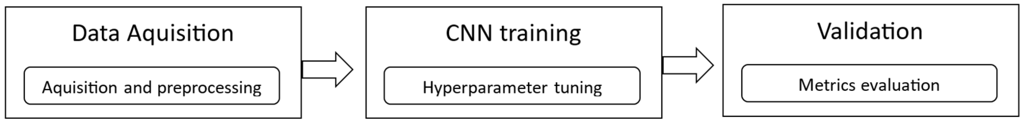
3. Materials and Methods

The methodology used in this study consists of three phases, as shown in Figure 3. The first phase describes the data acquisition procedure and the construction and general features of the obtained images. The second phase describes the transfer learning of CNN architectures used in this study and the configuration of hyperparameters, such as the learning rate, the lot size by iteration, the number of epochs, and the optimizer. The third phase describes the evaluation of the proposed models to measure the performance by applying different metrics.

Figure 3. Diagram of proposed methodology.

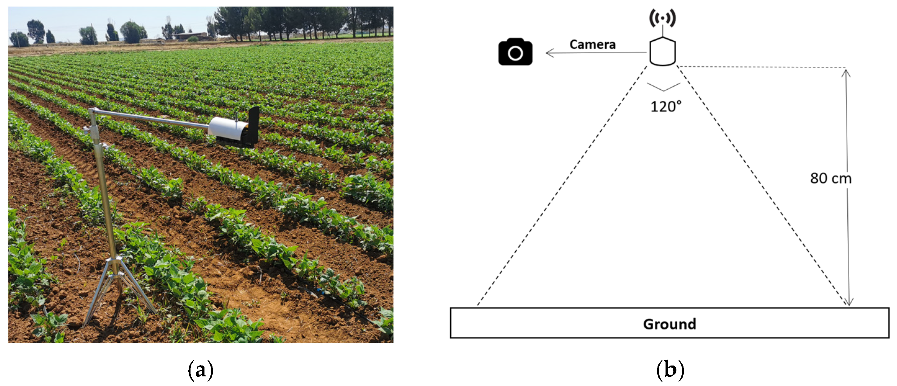
3.1. Acquisition of Data

The two selected bean parcels are located in the municipality of Calera de Víctor Rosales in the state of Zacatecas, Mexico (22°54′14.6″ N 102°39′32.5″ W). The variety of beans used was pinto Saltillo, and the data were collected between 12 May and 15 August of the year 2023. The camera model used was HC-801Pro, with 4G technology, a range of optical vision of 120°, IP65 protection, and a resolution of 30 megapixels to acquire high-quality images.

Two cameras were installed to capture the images, as shown in Figure 4. To determine the number of images for the training and testing data set, according to Tylor et al. [22], the average time for bean harvest after its emergence is from 65 to 85 days approximately, which is why an average of eight to ten images were captured per day since the emergence of the plant.

Figure 4. Installation of the GSM camera station in the open field for the capture of images: (a) camera station for the capture of images; (b) schematic diagram for the acquisition of images.

The shooting method used was for two samples per sequence for intervals of time between 8:00, 10:00, 12:00, 16:00, and 18:00 h, obtaining a total of 814 images, allowing the experimental data to include the bean growing cycle in the vegetative phase and the reproductive phase, from the germination phase of the plant (V0) through the emergence phase of the plant (V1), primary leaves (V2), the first trifoliate leaf (V3), the third trifoliate leaf (V4), prefloration (R5), floration (R6), pod formation (R8), pod filling (R8), and maturation (R9).

Generally, the bean’s phenology is classified into ten classes and divided into two main categories: the vegetative and the production phases. However, for this investigation, only four classes were selected according to the most significant number of examples per class since they tend to be the most representative, according to Etemadi et al. [39].

An example of each class of the obtained data set can be observed in Figure 5, labeling the vegetative phase in the stage of primary leaves, first and third trifoliate leaves (V2–V4), reproductive phase in the stage of prefloration and floration (R5–R6), reproductive phase in the stage of formation and filling of pods (R7–R8), and reproductive phase in the stage of maturation (R9).

Figure 5. Descriptive stages of the phenology of the bean: (a) vegetative phase in primary leaves, first and third trifoliate leaves; (b) reproductive phase in prefloration and floration; (c) reproductive stage in the formation and filling of pods; (d) reproductive phase in maturation.

The training data set and tests used per class can be observed in Figure 6. Most images have a resolution of 5120 × 3840 pixels. However, the images were re-dimensioned to adjust the size according to the entry specifications for each proposed model [34].

Figure 6. Images for training and tests per class.

3.2. Data Augmentation

The data augmentation contributes to avoiding overfitting the network and memorizing the exact details of the images during training. This is a common problem when the CNN model is exposed to small data sets where the learned patterns are not generalized into new data [40,41].

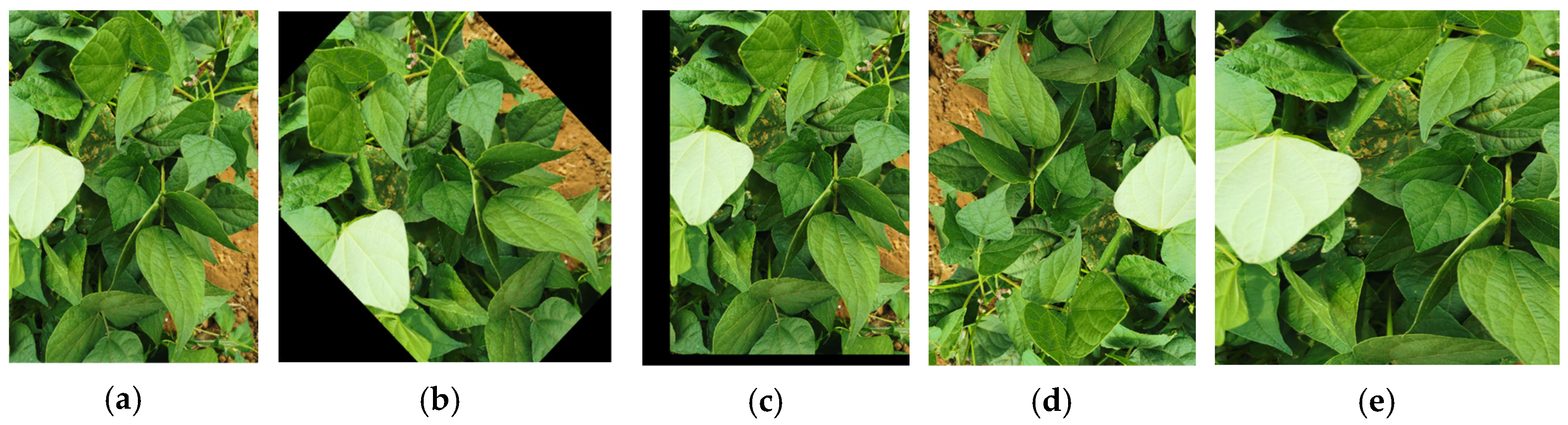
Currently, there is a tendency in deep learning training algorithms to allow for the increase of the initial data set through data augmentation techniques, obtaining results that can improve the precision performance in deep learning algorithms [42]. A series of aleatory transformations increased data to exploit the few examples of images and increase the precision of the proposed CNN models. The strategies of data augmentation used were rotation, translation, reflection, and scaling. Examples are shown in Figure 7.

Figure 7. Data augmentation in an image of the phenology of the bean: (a) original image without data increase; (b) image after rotation; (c) image after translation; (d) image after reflection; (e) image after scaling.

3.3. Training of the Models

For the training data set and tests, the images were divided randomly in a partition of 70% of the training data set and 30% for the test set. Table 2 shows the configuration of the experimental equipment used in this investigation. The four models previously selected were trained by the ImageNet database, which contains more than 15 million images [26].

Table 2. Configuration of experimental equipment.

Name of Configuration	Parameters
Processor	AMD Ryzen 7, 5700U, 8 cores at 1.8 GHz
Graphic Card	Radeon Graphics up to 4.3 GHz
RAM	16 GB
Operative system	Windows 11
Programing platform	MATLAB (2022a)

The hyperparameters selected in this study from the revised literature and the previously mentioned hardware capacity are described in Table 3. The selection of hyperparameters significantly affects the performance of CNN models, which is why a good selection is crucial. The hyperparameters were standardized for each model to compare the performance of the proposed models [31,43,44].

Table 3. Training hyperparameters of pre-trained models.

Re-Trained CNN Model	Image Size	Optimizer	Momentum	Epochs	Batch Size	Learning Rate
AlexNet	227 × 227	Stochastic Gradient Descent with Momentum	0.9	15	128	0.001
VGG19	224 × 224
SqueezeNet	227 × 227
GoogleNet	224 × 224

The optimizer used is the Stochastic Gradient Descent with Momentum (SGDM) method, which combines stochastic gradient descent and momentum techniques. Each iteration calculates the gradient using a random sample from the training set. Then, the weight is updated considering the previous update, allowing convergence acceleration and keeping it at a local minimum.

Momentum is employed to improve the precision and velocity of the training by adding a fraction from the previous step to the present step in the weight update. This allows it to overcome the obstacle of local minimums and maintain a constant impulse in the direction of the gradient.

The epochs refer to the number of iterations carried out regarding the correlation of forward and reverse propagation to reduce loss. The size of the epochs describes the number of examples used in each iteration of the training algorithm. The learning rate is defined by the velocity size in which the optimization function performs a search to converge [45].

3.4. Performance Evaluation

At present, an extended variety of metrics are used to evaluate the performance of CNN models, where information is given about the aspects and characteristics that allow the evaluation of the performance of the models. A number of true positives (TP), true negatives (TN), false positives (FP), and false negatives (FN) are needed to calculate the performance of the models. These cases represent the combinations of true and predicted classes in classification problems. Therefore, TP + TN + FP + FN equals the total number of samples and is described in a confusion matrix [46].

When trained by transfer learning, the biased distributions appear naturally, producing an intrinsic unbalance. This is why it is necessary to employ metrics that evaluate the global performance of each model. In this regard, the metrics employed [16,20,22,46,47] were used to compare the performance of the models without setting aside the different characteristics of the training and validation data used in this study.

TP is the true positive, which means the prediction is positive. FP is the false positive, which means the prediction is negative. However, the prediction is positive. FN is the false negative, which means a positive prediction, but the result is negative. TN is the true negative, which means a negative result prediction.

The confusion matrix is a tool that allows the visualization of a model’s performance when classifying and containing the previously defined elements. The rows in the matrix represent the true class, and the columns, the predicted class, and the primary diagonal cells describe the correctly classified observations. In contrast, the lateral diagonals correspond to the incorrectly classified observations.

In this study, five metrics were used to evaluate the performance of the proposed models: accuracy, precision, sensitivity, specificity, and F1-Score [27,48]. Accuracy is the relation between the number of correct predictions and the total number of made predictions, as calculated by Equation (1).

$$\mathrm{A}\mathrm{c}\mathrm{c}\mathrm{u}\mathrm{r}\mathrm{a}\mathrm{c}\mathrm{y}=\frac{\mathrm{T}\mathrm{P}+\mathrm{T}\mathrm{N}}{\mathrm{T}\mathrm{P}+\mathrm{T}\mathrm{N}+\mathrm{F}\mathrm{P}+\mathrm{F}\mathrm{N}}$$

(1)

Precision measures the proportion of correct predictions made by the model, in other words, the number of correctly classified elements as positives out of a total of elements identified as positive. The mathematical representation is described in Equation (2).

$$\mathrm{P}\mathrm{r}\mathrm{e}\mathrm{c}\mathrm{i}\mathrm{s}\mathrm{i}\mathrm{o}\mathrm{n}=\frac{\mathrm{T}\mathrm{P}}{\mathrm{T}\mathrm{P}+\mathrm{F}\mathrm{P}}$$

(2)

Sensitivity is also known as recall; it calculates the proportion of correctly identified cases as positive from a total of true positives, as described in Equation (3).

$$\mathrm{S}\mathrm{e}\mathrm{n}\mathrm{s}\mathrm{i}\mathrm{t}\mathrm{i}\mathrm{v}\mathrm{i}\mathrm{t}\mathrm{y}=\frac{\mathrm{T}\mathrm{P}}{\mathrm{T}\mathrm{P}+\mathrm{F}\mathrm{N}}$$

(3)

Specificity is the opposite of sensitivity or recall and calculates the portion of cases identified as negatives. It is calculated by Equation (4).

$$\mathrm{S}\mathrm{p}\mathrm{e}\mathrm{c}\mathrm{i}\mathrm{f}\mathrm{i}\mathrm{c}\mathrm{i}\mathrm{t}\mathrm{y}=\frac{\mathrm{T}\mathrm{N}}{\mathrm{T}\mathrm{N}+\mathrm{F}\mathrm{P}}$$

(4)

F1-Score allows the combination of precision and sensitivity or recall, where the value of one indicates a good balance between precision and sensitivity in the classification model. Its mathematical representation is described in Equation (5).

$$\mathrm{F}1\text{-}\mathrm{s}\mathrm{c}\mathrm{o}\mathrm{r}\mathrm{e}=2\times \frac{\mathrm{p}\mathrm{r}\mathrm{e}\mathrm{c}\mathrm{i}\mathrm{s}\mathrm{i}\mathrm{o}\mathrm{n}\times \mathrm{r}\mathrm{e}\mathrm{c}\mathrm{a}\mathrm{l}\mathrm{l}}{\mathrm{p}\mathrm{r}\mathrm{e}\mathrm{c}\mathrm{i}\mathrm{s}\mathrm{i}\mathrm{o}\mathrm{n}+\mathrm{r}\mathrm{e}\mathrm{c}\mathrm{a}\mathrm{l}\mathrm{l}}$$

(5)

4. Results and Discussion

Table 4 provides a detailed calculation for each of the different metrics of AlexNet’s architecture. A sensitivity of 100% was obtained for the prediction of classes R9 and V2–V4, which correspond to the reproductive phenological phase in the stage of maturation and the vegetative phase in the stage of primary leaves and first and third trifoliate leaves, respectively.

Table 4. Calculation of metric for the AlexNet model.

Name	Classes				Averaging
True Positive	62	93	23	55	58.25
False Positive	3	2	4	1	2.5
False Negative	2	8	0	0	2.5
True Negative	176	140	216	187	179.75
Accuracy	0.958847	0.958847	0.958847	0.958847	0.958847
Precision	0.953846	0.978947	0.851851	0.982142	0.941697
Sensitivity	0.968750	0.920792	1	1	0.972385
Specificity	0.983240	0.985915	0.981818	0.994680	0.986413
F1-Score	0.961240	0.948979	0.920000	0.990990	0.955302

The averages obtained for the accuracy, precision, sensitivity, specificity, and F1-Score were 95.8%, 94.1%, 97.2%, 98.6%, and 95.5% of the predicted classes during validation, respectively.

Table 5 shows the different metrics in the VGG19 model. In classes R5-R6, corresponding to the reproductive phenological phase in the stages of prefloration and floration, a precision of 100% was reached.

Table 5. Calculation of metrics for VGG19 model.

Name	Classes				Averaging
True Positive	60	97	23	55	58.75
False Positive	0	3	4	1	2
False Negative	4	4	0	0	2
True Negative	179	139	216	187	180.25
Accuracy	0.967078	0.967078	0.967078	0.967078	0.967078
Precision	1	0.970000	0.851851	0.982142	0.950998
Sensitivity	0.937500	0.960396	1	1	0.974474
Specificity	1	0.978873	0.981818	0.994680	0.988843
F1-Score	0.967741	0.965174	0.920000	0.990990	0.960976

A 95% precision average for all classes can be observed. On the other hand, maximum sensitivity was also obtained for classes R9 and V2–V4, corresponding to the phenological phase of reproduction in the maturation stage and vegetative phase of primary leaves and first and third trifoliate leaves, respectively. An average of 97.4% of sensitivity is observed in each class. In addition, averages reached for specificity are 98.8% and 96% F1-Score in all classes, achieving the best scores compared to the other architectures.

A detailed calculation for each metric used in the architecture SqueezeNet can be shown in Table 6. For the classes V2–V4, which corresponds to the vegetative phenological phase in the stage of primary leaves and first and third trifoliate leaves, a sensitivity of 100% was obtained. On the other hand, averages in accuracy, precision, sensitivity, and F1-Score of 95.8%, 93.4%, 95.9%, 98.6%, and 94.4%, respectively, are observed for all predicted classes during validation.

Table 6. Calculation of metrics for SqueezeNet model.

Name	Classes				Averaging
True Positive	59	97	22	55	58.25
False Positive	0	3	6	1	2.50
False Negative	5	4	1	0	2.50
True Negative	179	139	214	187	179.75
Accuracy	0.958847	0.958847	0.958847	0.958847	0.958847
Precision	1	0.970000	0.785714	0.982142	0.934464
Sensitivity	0.921875	0.960396	0.956521	1	0.959698
Specificity	1	0.978873	0.972727	0.994680	0.986570
F1-Score	0.959349	0.965174	0.862745	0.990990	0.944564

The different metrics of the GoogleNet model can be observed in Table 7, where the average obtained for precision is 96.8% in all predicted classes, and there is a maximum sensitivity in the prediction of classes V2–V4 that corresponds to the vegetative phenological phase in the stage of primary leaves and first and third trifoliate leaves. The averages observed in the metrics of accuracy, precision, sensitivity, specificity, and F1-Score are 96.7%, 96.8%, 95.7%, 98.7%, and 96.2%, respectively, for all predicted classes during validation, which concur with the metric of precision obtained for the VGG19 model.

Table 7. Calculation of metrics for GoogleNet model.

Name	Classes				Averaging
True Positive	60	99	21	55	58.75
False Positive	1	5	1	1	2
False Negative	4	2	2	0	2
True Negative	178	137	219	187	180.25
Accuracy	0.967078	0.967078	0.967078	0.967078	0.967078
Precision	0.983606	0.951923	0.954545	0.982142	0.968054
Sensitivity	0.937500	0.980198	0.913043	1	0.957685
Specificity	0.994413	0.964788	0.995454	0.994680	0.987334
F1-Score	0.960000	0.965853	0.933333	0.990990	0.962544

Table 8 shows the results obtained in each metric, with the best values obtained during the architecture’s evaluation highlighted in bold. It shows that the architecture of VGG19 and GoogleNet obtained the best performance, and both concur in accuracy. On the other hand, the architecture with the lowest performance observed is SqueezeNet due to the values obtained that are generally lower than those obtained in other architectures. However, SqueezeNet required the least training time in comparison to the others.

Table 8. Comparison of results for each of the architectures.

Metrics	AlexNet	VGG19	SqueezeNet	GoogleNet
Accuracy	0.9588	0.9671	0.9588	0.9671
Precision	0.9417	0.9510	0.9345	0.9681
Sensitivity	0.9724	0.9745	0.9597	0.9577
Specificity	0.9864	0.9888	0.9866	0.9873
F1-Score	0.9553	0.9610	0.9446	0.9625
Time [minutes]	17.31	168.76	20.19	25.48

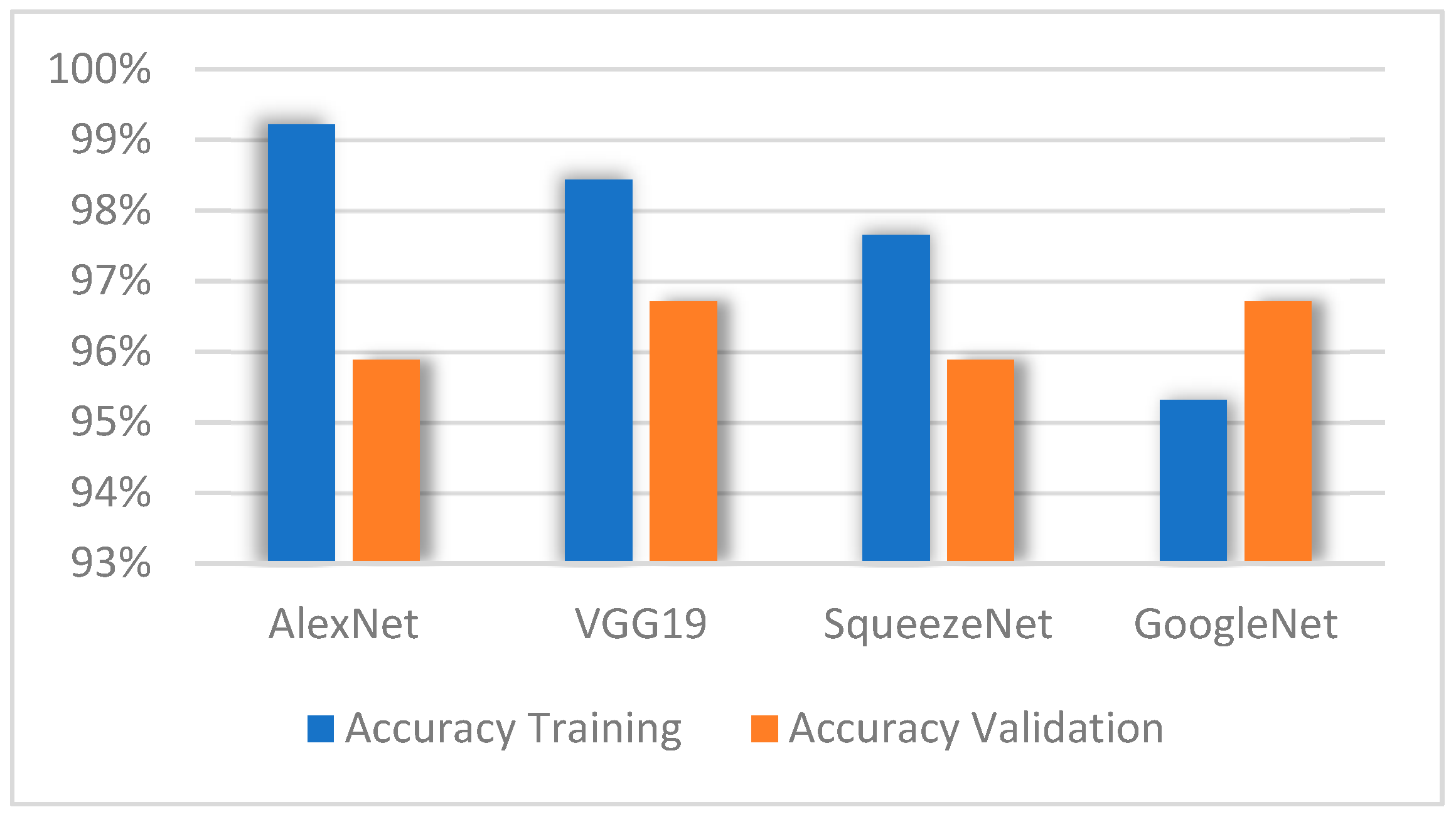
A comparison of the accuracy obtained in each of the models during the training and validation stages is shown in Figure 8, where the architecture AlexNet reaches the highest accuracy percentage compared to the other models during the training stage. However, in the validation stage, VGG19 reached the highest accuracy percentage. This stage shows that the GoogleNet model obtained the lowest accuracy percentage compared to the other models. However, it is observed that this model reached the highest accuracy percentage during the validation stage, just like VGG19; in other words, they obtained a greater capacity.

Figure 8. Accuracy of models during training and validation.

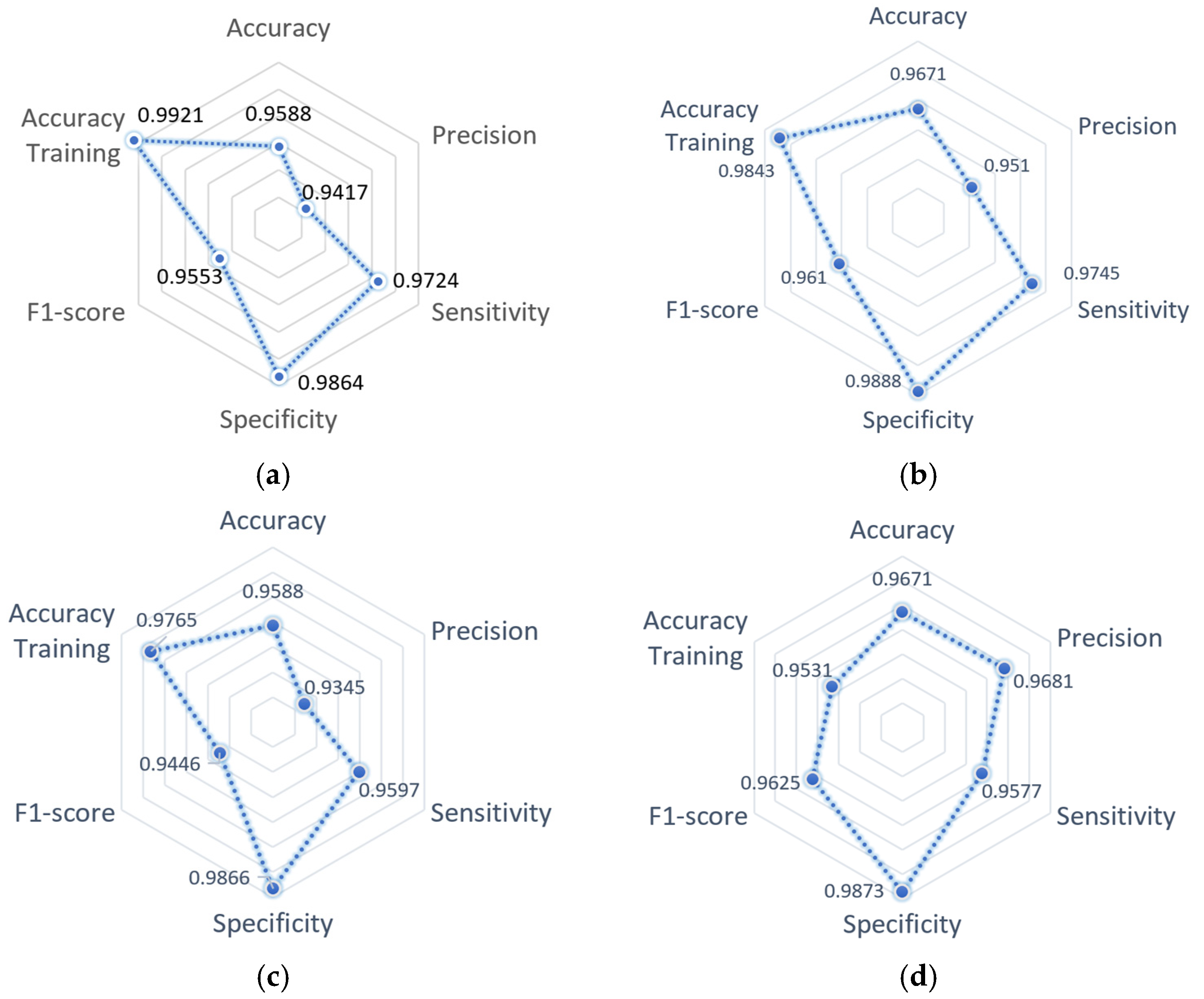
The architecture performance summary with measurements obtained in each metric calculated during the validation stage can be observed in Figure 9; the accuracy metric obtained during the training stage is included for each model. It is observed that the GoogleNet architecture maintained the best balance in the projection of all metrics. On the other hand, it is observed that the architecture SqueezeNet obtained the best performance compared to the rest of the architectures, except in precision, where the result is the same as the AlexNet architecture, and sensitivity is less than the obtained with the GoogleNet architecture.

Figure 9. Summary of model performance: (a) AlexNet model; (b) VGG19 model; (c) SqueezeNet model; (d) GoogleNet model.

Based on the obtained results, the GoogleNet architecture has a higher performance during the validation compared to its performance during the training process; the cause of this behavior could be due to the limited amount of training data, the adequate selection of hyperparameters, and possibly an over-adjustment. However, the difference between the precision of training and validation is 1.4% compared to the models AlexNet, VGG19, and SqueezeNet, which present a difference of 1.7%, 3.3%, and 1.7%, respectively—considering that increased training data will give an outcome with a tendency to decrease the performance during the validation of each architecture.

According to the behavior during the validation, the architectures AlexNet and SqueezeNet presented a low-balanced tendency in the metrics, obtaining low results for precision and F1-Score. On the other hand, the architecture VGG19 registered the same level of performance as GoogleNet but with lower precision and F1-Score, giving a reason to consider the architecture GoogleNet as having the best global performance.

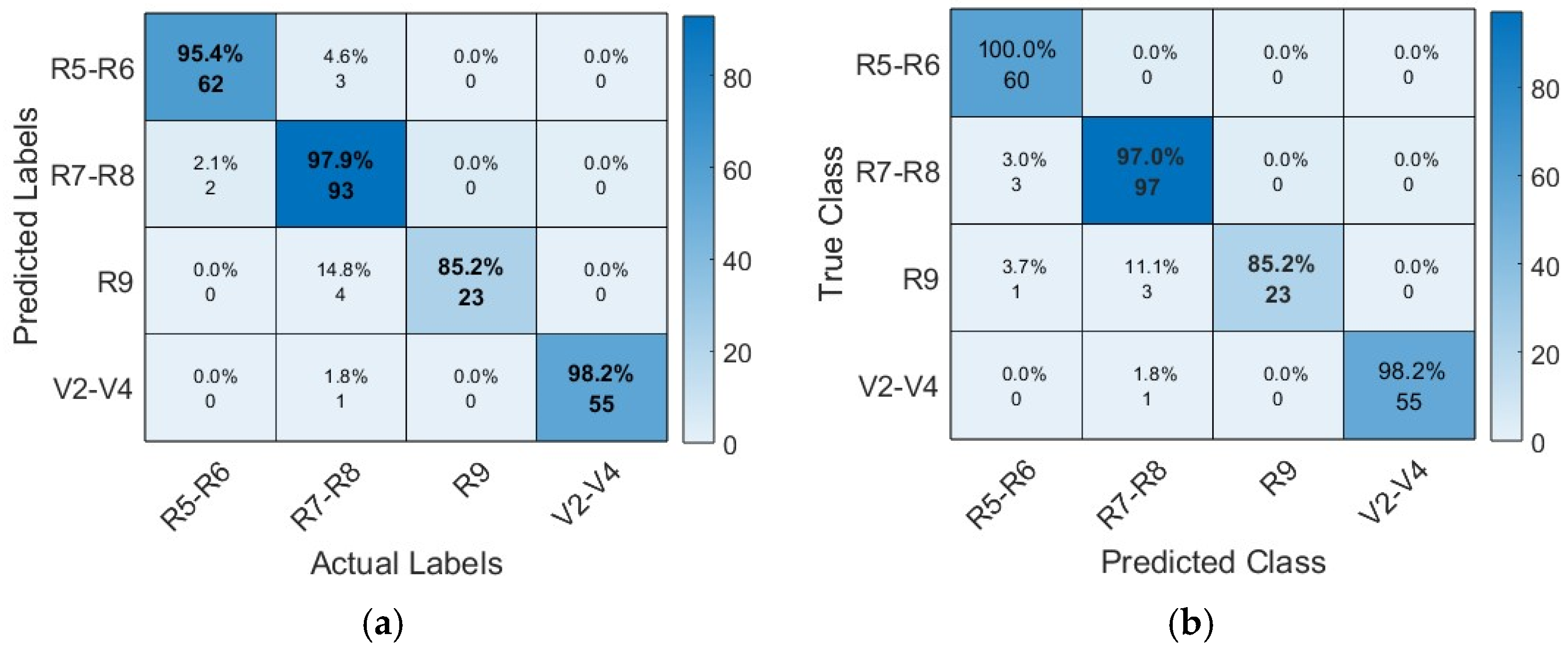
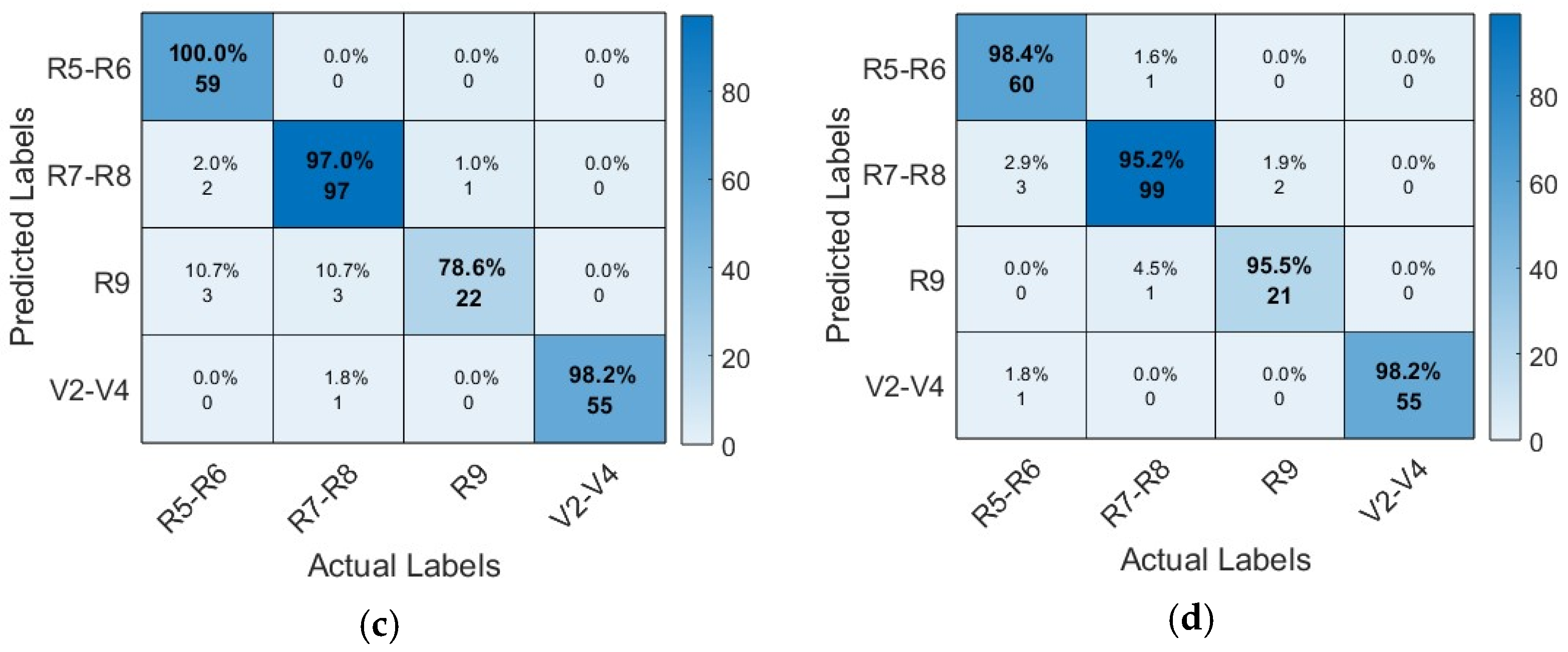
Figure 10 shows the confusion matrix of the four proposed CNN models. It also provides a detailed analysis of instance numbers correctly classified by each proposed architecture. Compared to other architectures, the AlexNet architecture presented problems in correctly classifying the class R9, which corresponds to the reproductive phenological phase in the stage of maturation, achieving the classification of only 85.2% of instances.

Figure 10. Confusion matrix of CNN models: (a) AlexNet architecture; (b) VGG19 architecture; (c) SqueezeNet architecture; (d) GoogleNet architecture.

The confusion matrix of the VGG19 architecture shows its high capacity to classify instances correctly. The diagonal shows the correctly classified instances; however, class R9 presented the most difficulty. The SqueezeNet architecture, like the previous architectures, shows more difficulties in correctly classifying the class R9; however, for the GoogleNet architecture, the class presents minimal difficulties.

Table 9 describes a comparison summary of the performance results obtained by other authors concerning the techniques and metrics used for this work. It breaks down the values obtained for accuracy, precision, sensitivity, and F1-Score for each proposed architecture.

Table 9. Comparison of similar work recently published.

Author	Phenology	Technique	Data Augmentation	Accuracy [%]	Precision [%]	Sensitivity [%]	F1-Score [%]
Yalcin [16]	Wheat, barley, lentil, cotton, and pepper	Re-trained CNN AlexNet model	Not	87.14	88.12	87.24	87.28
Qin et al. [46]	Rice	Re-trained CNN ResNet-50 model	Yes	87.33	-	-	-
Reeb et al. [20]	Alliaria petiolata	Re-trained CNN ResNet-18 model	Not	86.4	-	-	-
Taylor et al. [22]	Corn, wheat, barley, soybean, and alfalfa	Re-trained CNN VGG16 model and temporal model of Markov	Not	-	92	90	91
Han et al. [47]	Rice	CNN model with support vector machine (SVM)	Yes	91.3	-	-	93
This study	Bean	Re-trained CNN GoogleNet model	Yes	96.71	95.1	97.45	96.1

5. Conclusions

The proposed methodology shows that the proposed CNN models allow the correct classification of more than 90% of the samples, even when working with an unbalanced and relatively minor data set. In addition, each analyzed architecture has different characteristics, such as the number of layers and used filters. However, it is crucial to highlight a suitable selection of metrics to discriminate one architecture from the other.

Evaluating different CNN topologies is significant for future work since the architectures can present bias due to being trained with numerous images from which many are not part of the final classification. In this regard, evaluating the performance by transfer with new data lays the foundation for new work, such as identifying nutrients or plagues for this species. The joint evaluation of the metrics accuracy, precision specificity, sensitivity, and F1-Score allows the obtention of a multifaceted analysis, resulting in a higher performance GoogleNet architecture. Even though the global performance of each model is acceptable, data augmentation can modify the performance of all architectures.

One of the main limitations in the implementation of CNN models is the lack of data for certain classes, for which the main contribution of this study is to be able to distinguish the performance obtained through a reduced data set, where the application of data augmentation techniques other than reducing the overfitting in training helps improve the capacity of generalization in the network in comparison to other studies where augmentation techniques were not applied in the same way as the performance results of the models in Table 9.

On the other hand, through a methodological analysis, the performance was compared and evaluated by applying five metrics to four CNN models. The GoogleNet architecture obtained the best performance, showing the best results in most metrics, obtaining 96.71% accuracy, 96.81% precision, 95.77% sensitivity, 98.73% specificity, and 96.25% F1-Score.

6. Future Work

This study will open other alternatives that could be applied using the same transfer-by-learning approach for the controlled prevention of plagues and diseases in bean crops through timely intervention and automated computerized image classification.