


Enhanced Deep Learning Architecture for Rapid and Accurate Tomato Plant Disease Diagnosis

 ,
, 
 ,
,  and
and
Abstract
1. Introduction
2. Related Works
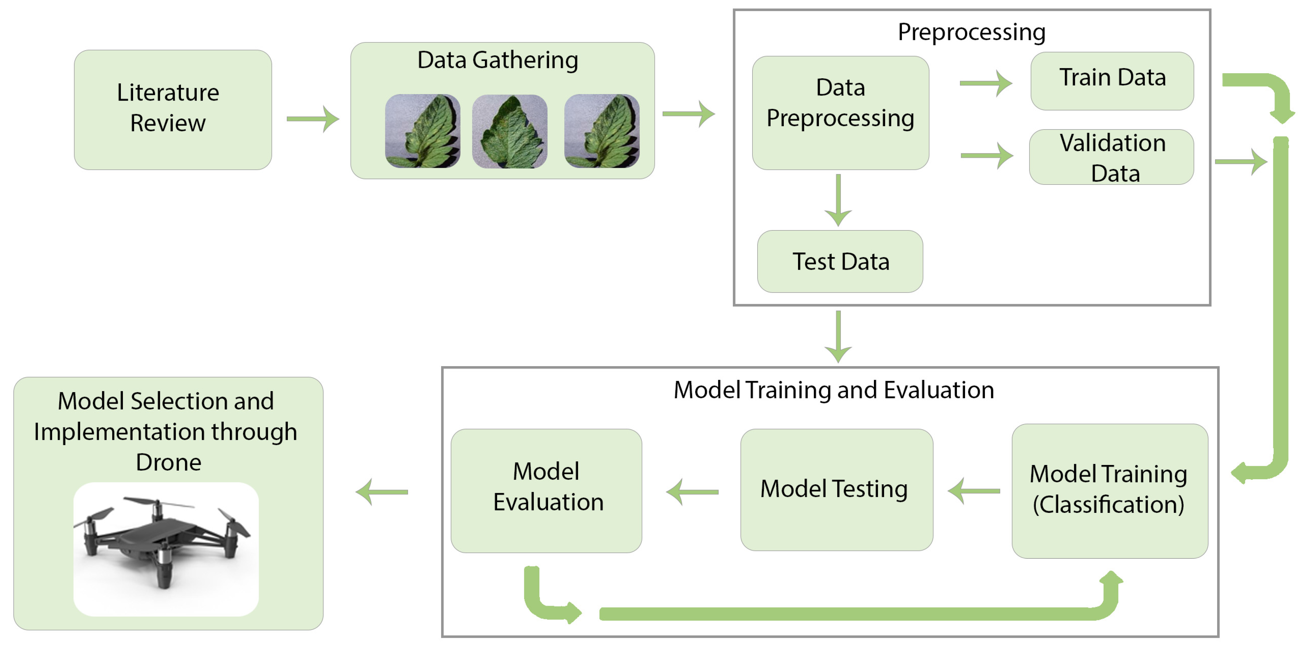
3. Methods and Data Collection
3.1. Data Collection
3.2. Data Preprocessing
3.3. Data Cleaning
3.4. Data Splitting
3.5. Data Augmentation
- Resize and Rescale
- Data Prefetch
- Label Encoding
- Term Frequency Inverse Document Frequency
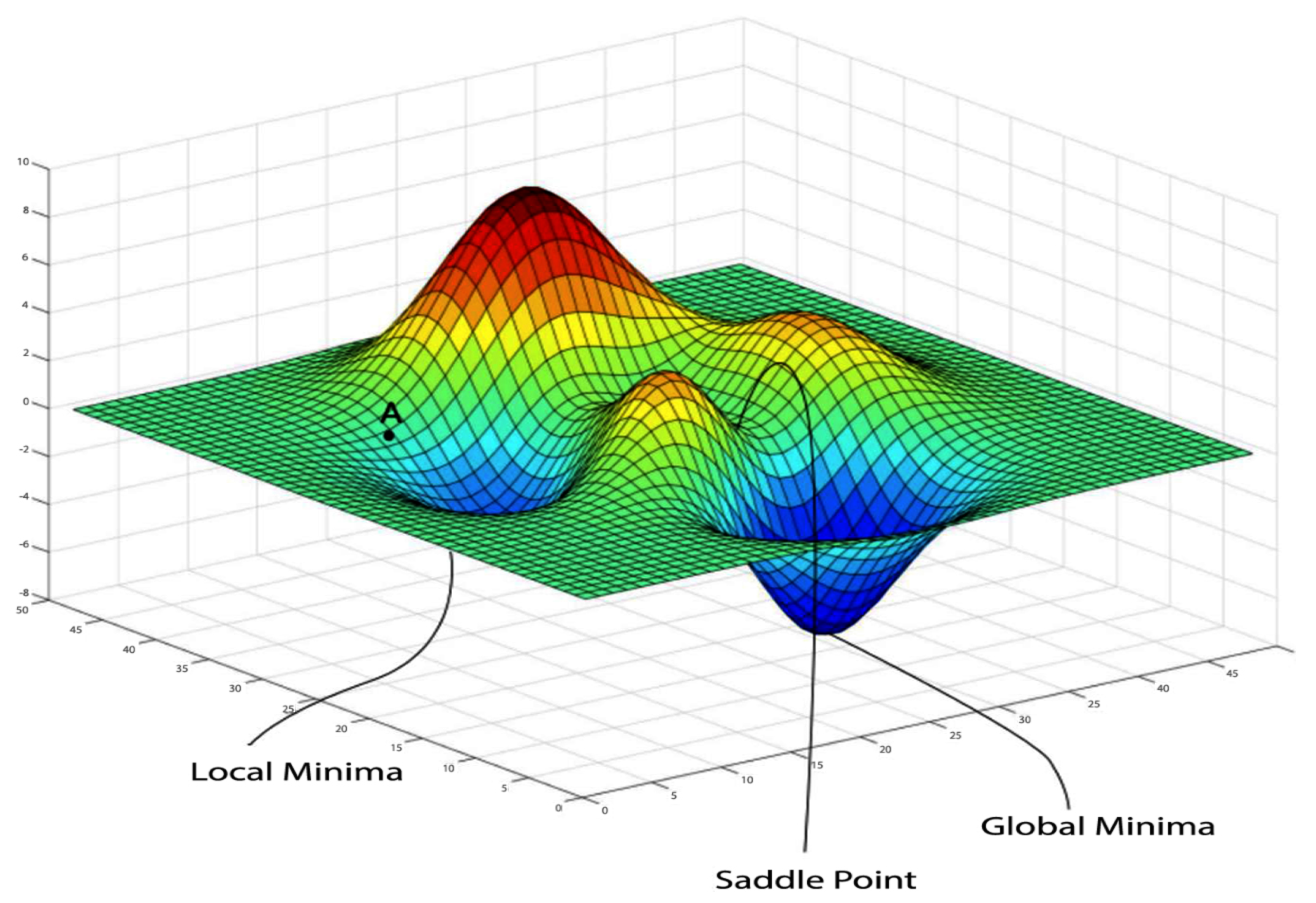
3.6. Model Training
3.7. Model Testing
3.8. Model Selection
3.9. Implementation and Experimental Setup
3.10. Deep Learning Architecture
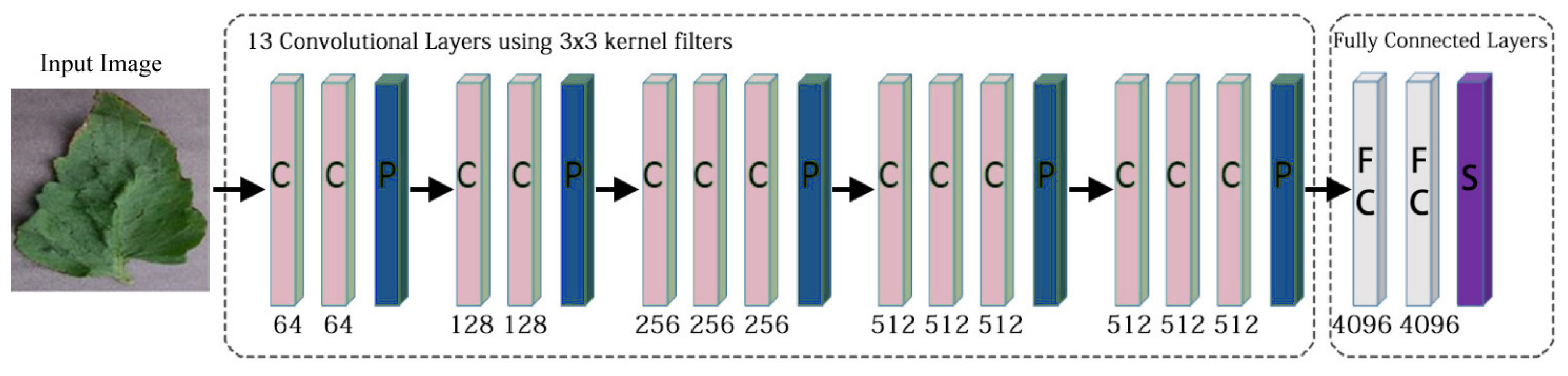
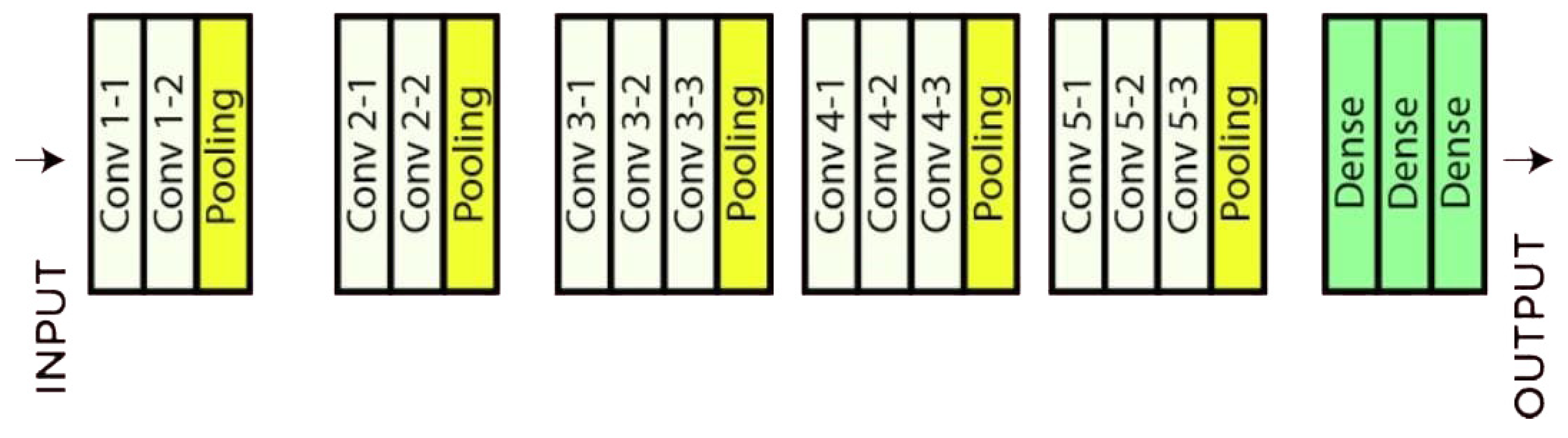
3.11. Visual Geometry Group (VGG)
3.12. Custom Model
- The first layer has 16 filters and a kernel size of 3 × 3.
- These layers have an average pooling of 2 × 2.
- The second and third layer has 32 filters and a kernel size of 3 ×3.
- These layers have an average pooling of 2 × 2.
- The fourth to sixth layer has 64 filters and a kernel size of 3 × 3.
- These layers have an average pooling of 2 × 2.
- The seventh to tenth layer has 512 filters and a kernel size of 3 × 3.
- These layers have an average pooling of 2 × 2.
- The first Dense layers have units of 256.
- The second Dense layers have units of 64.
- The third Dense layers have units of 32.
4. Results
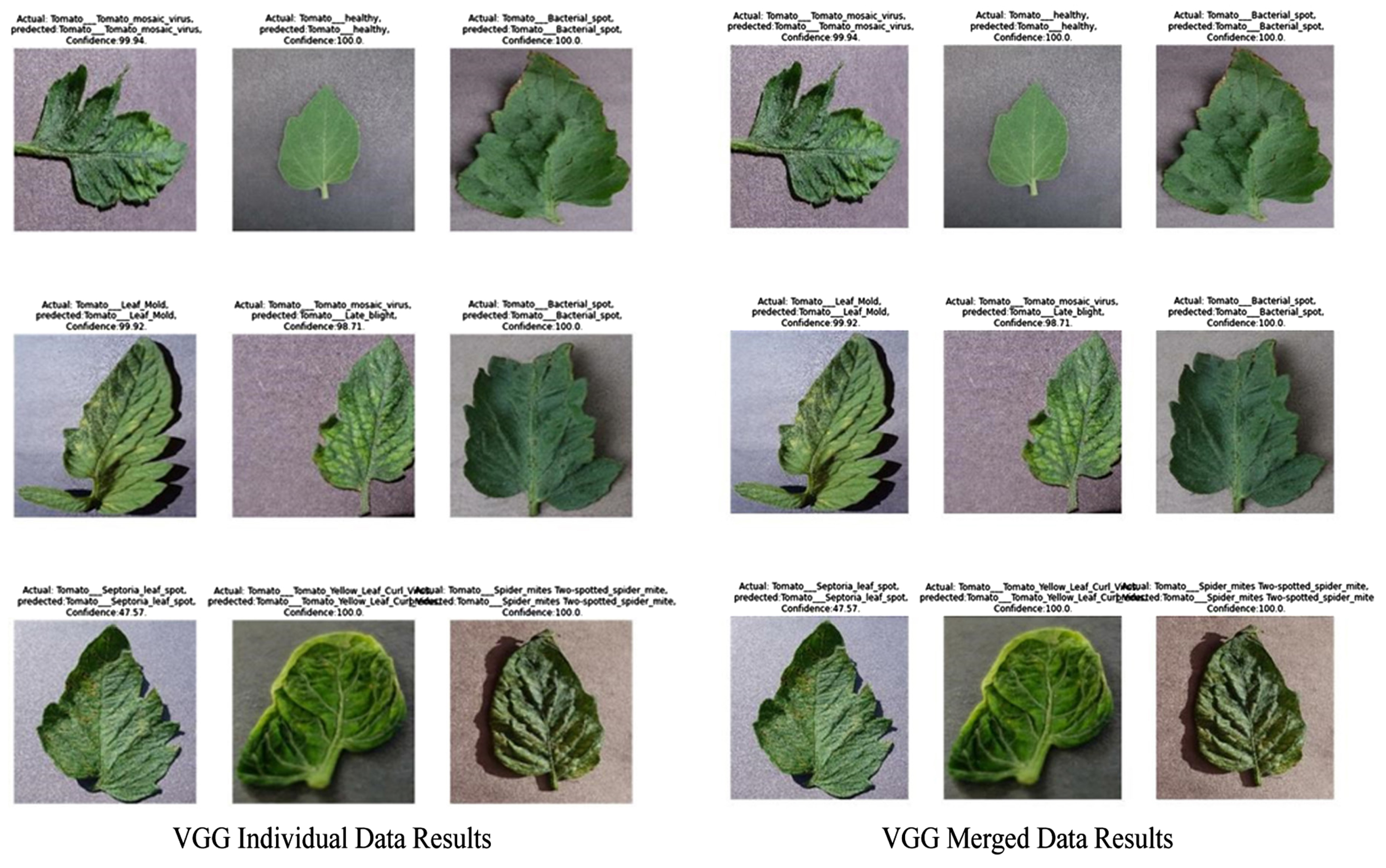
4.1. Visual Geometry Group 16
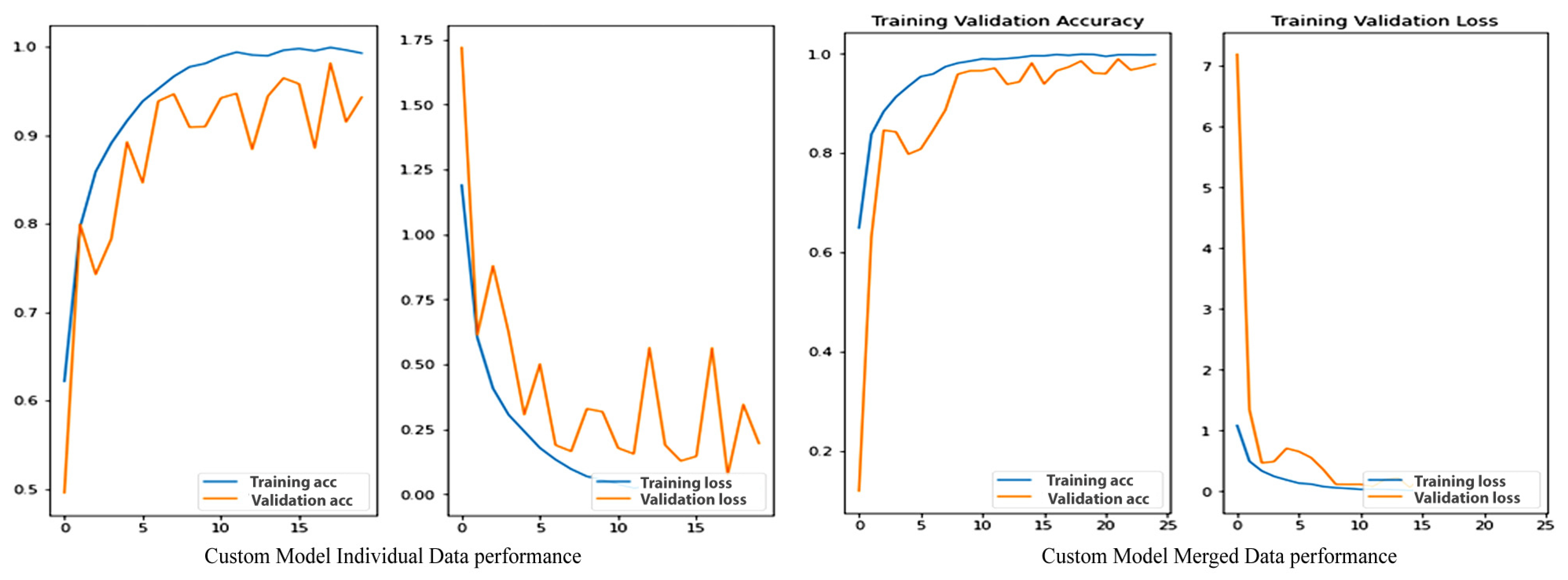
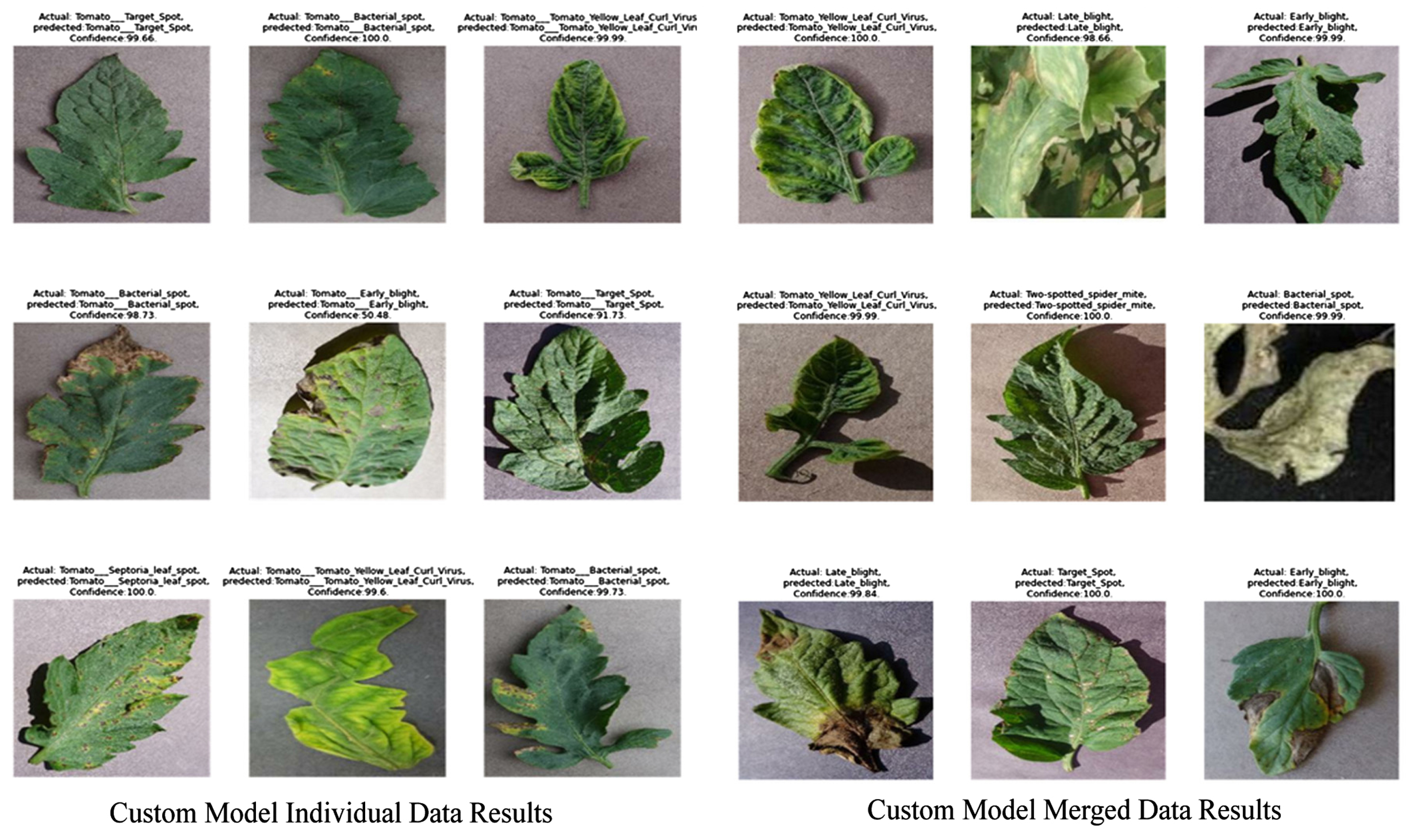
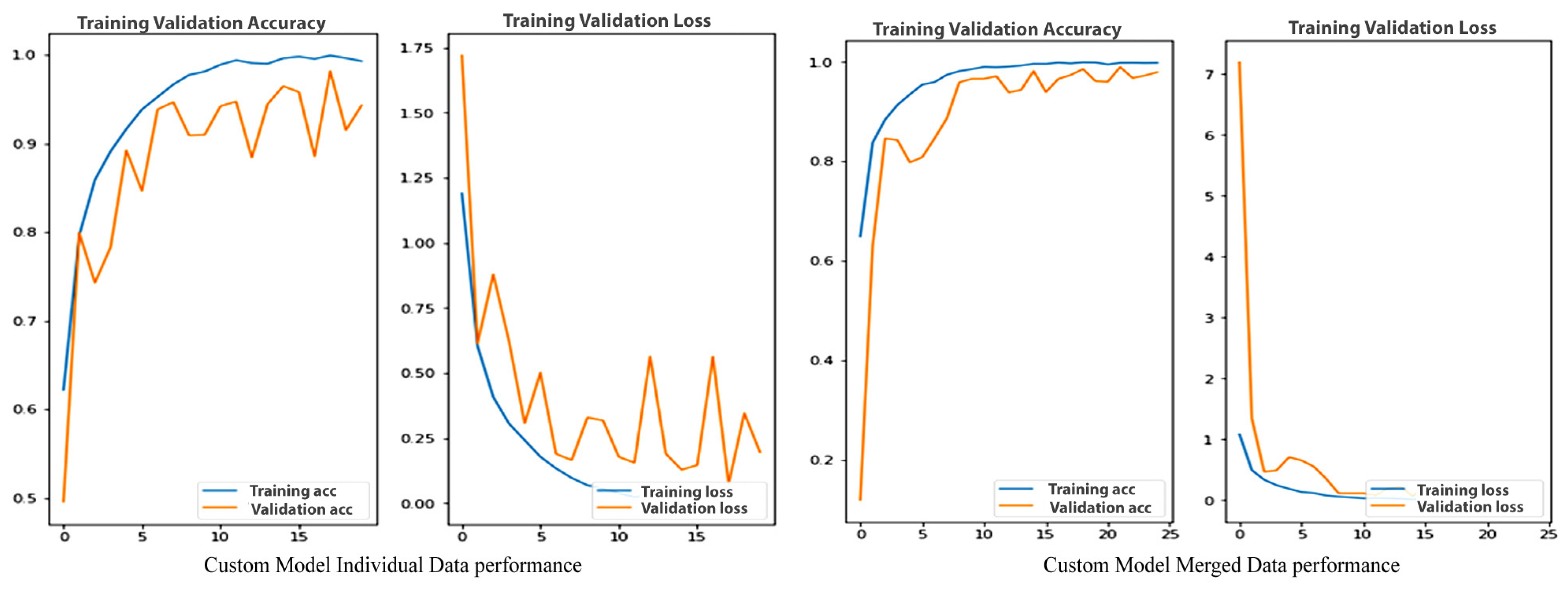
4.2. Custom Model
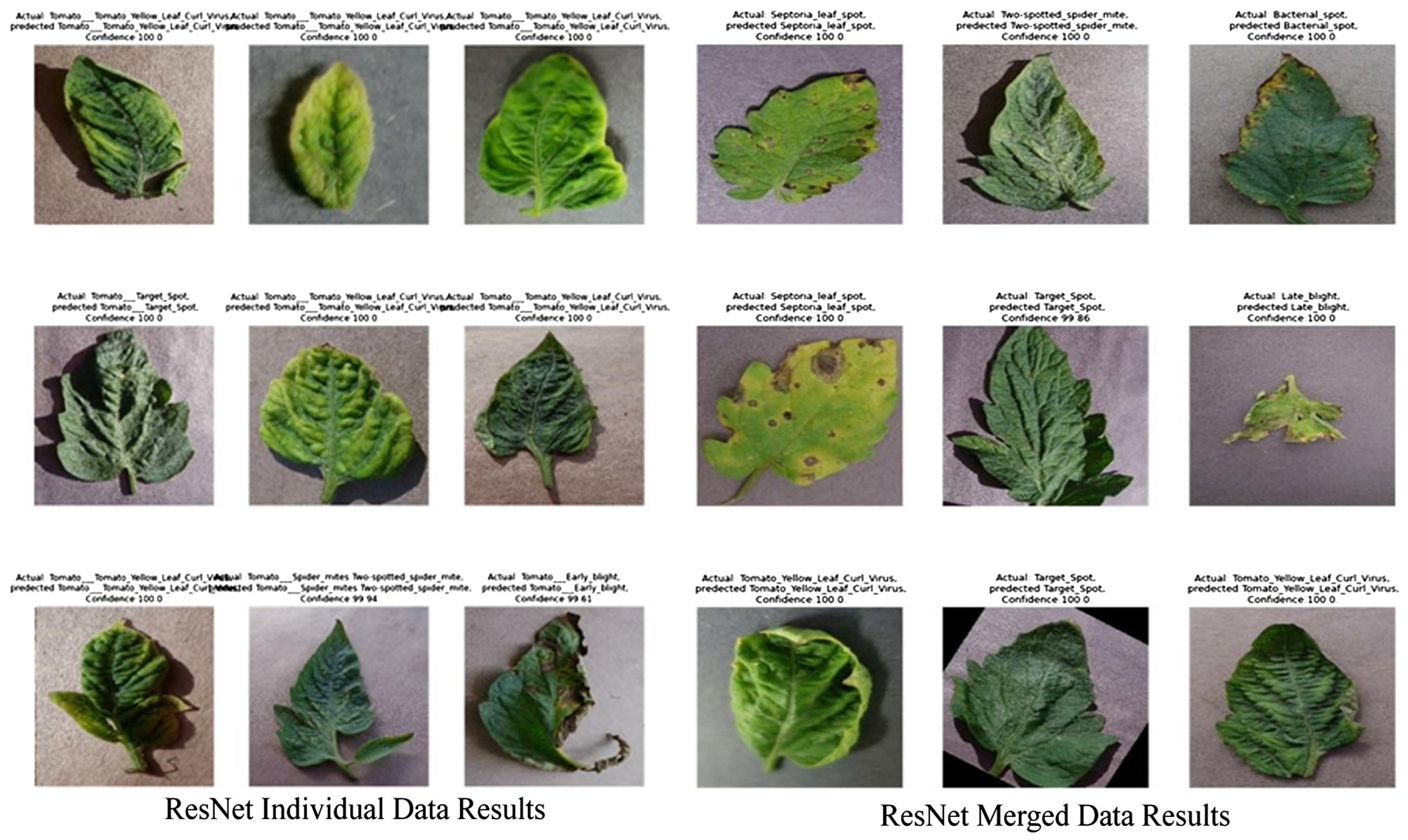
4.3. Residual Net
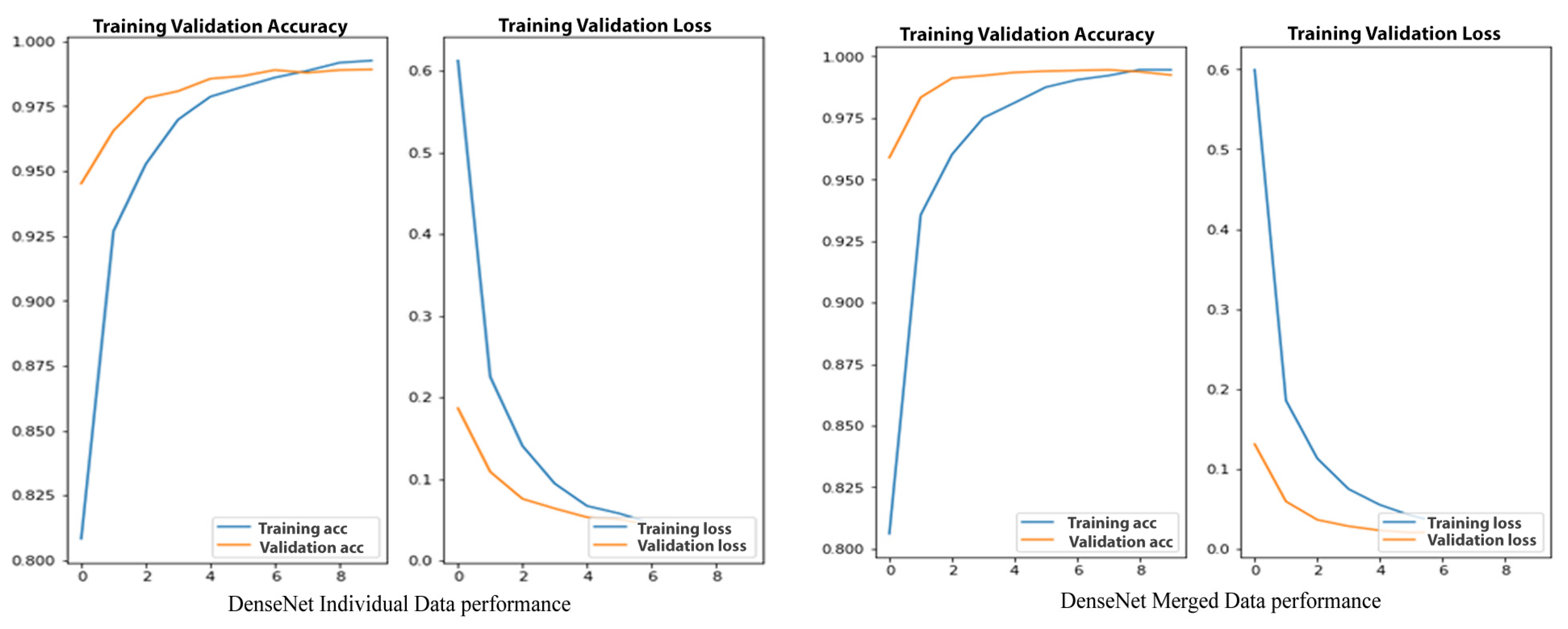
4.4. DenseNet121
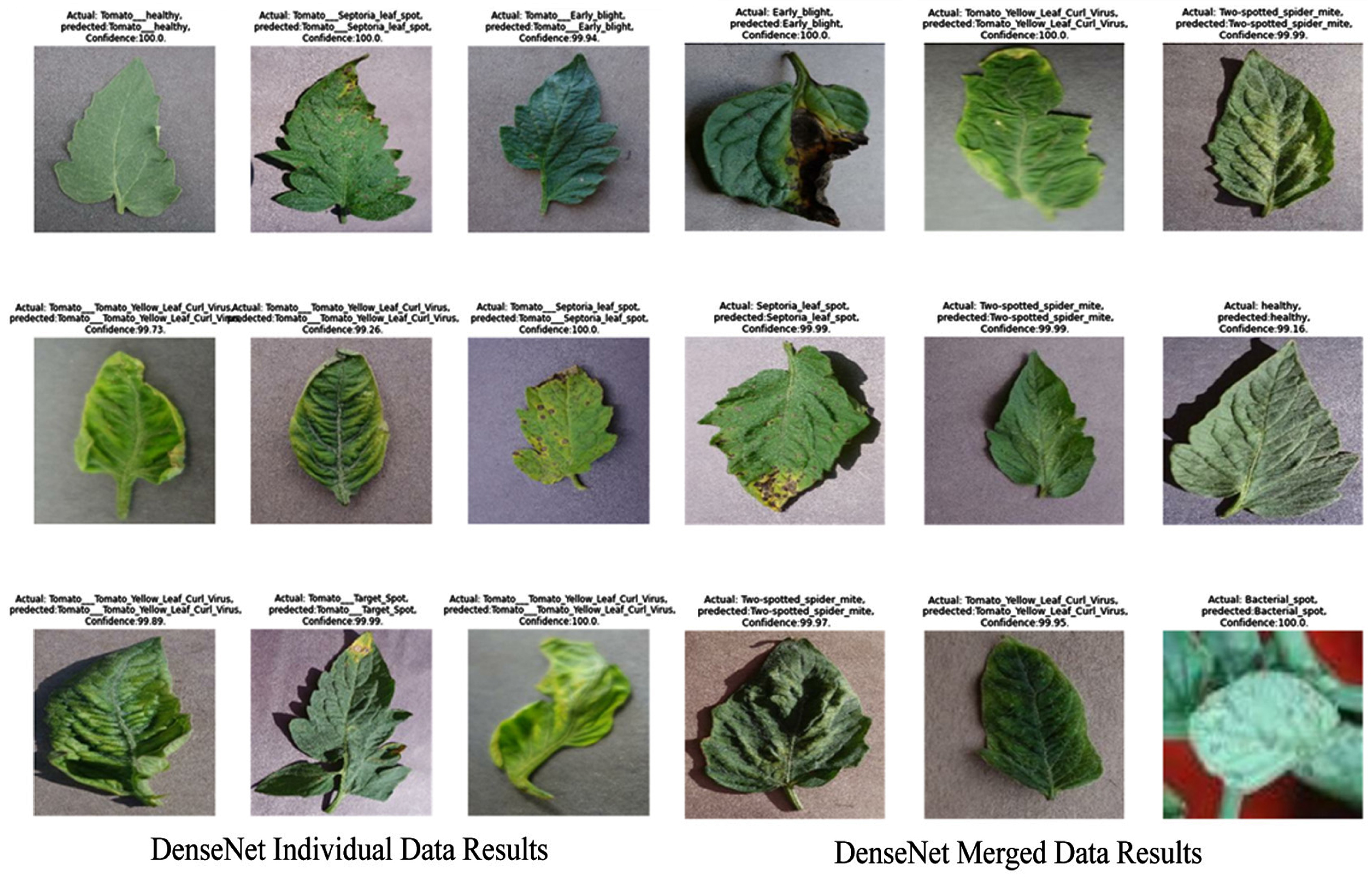
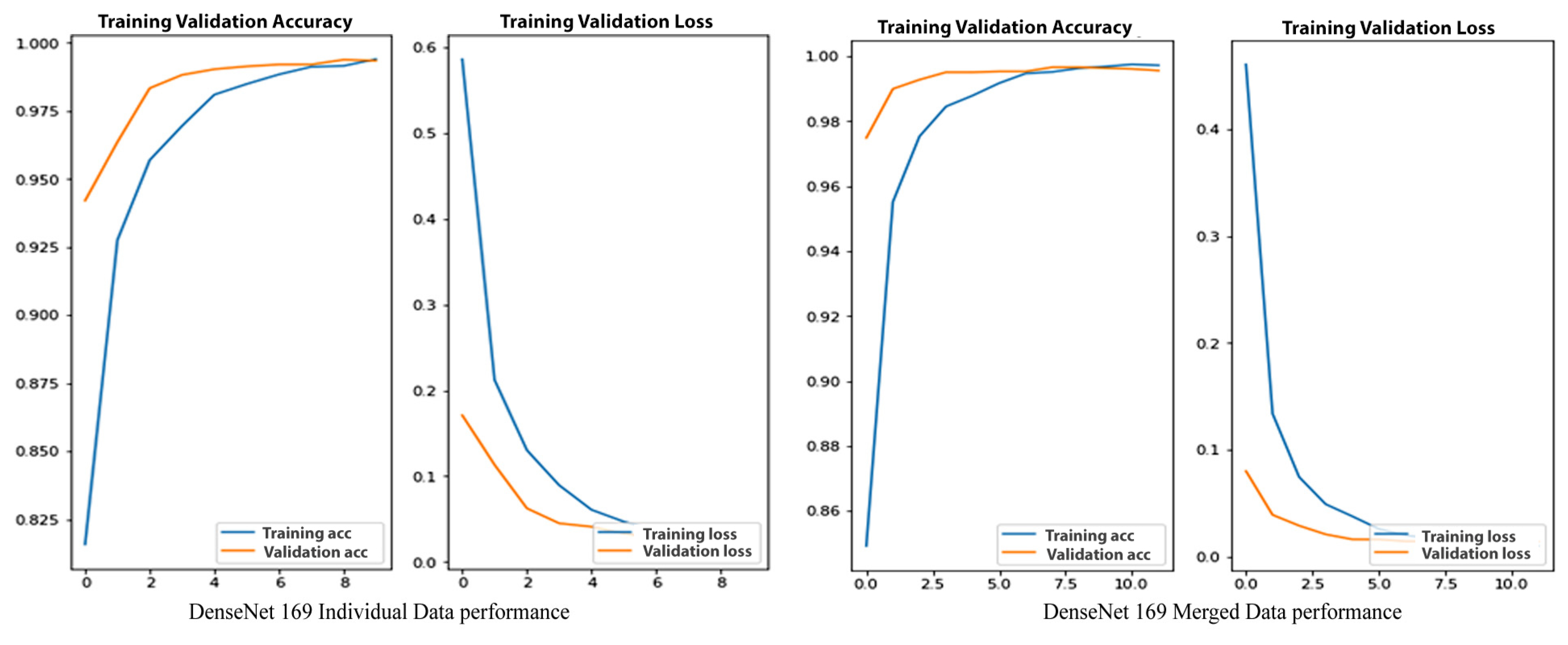
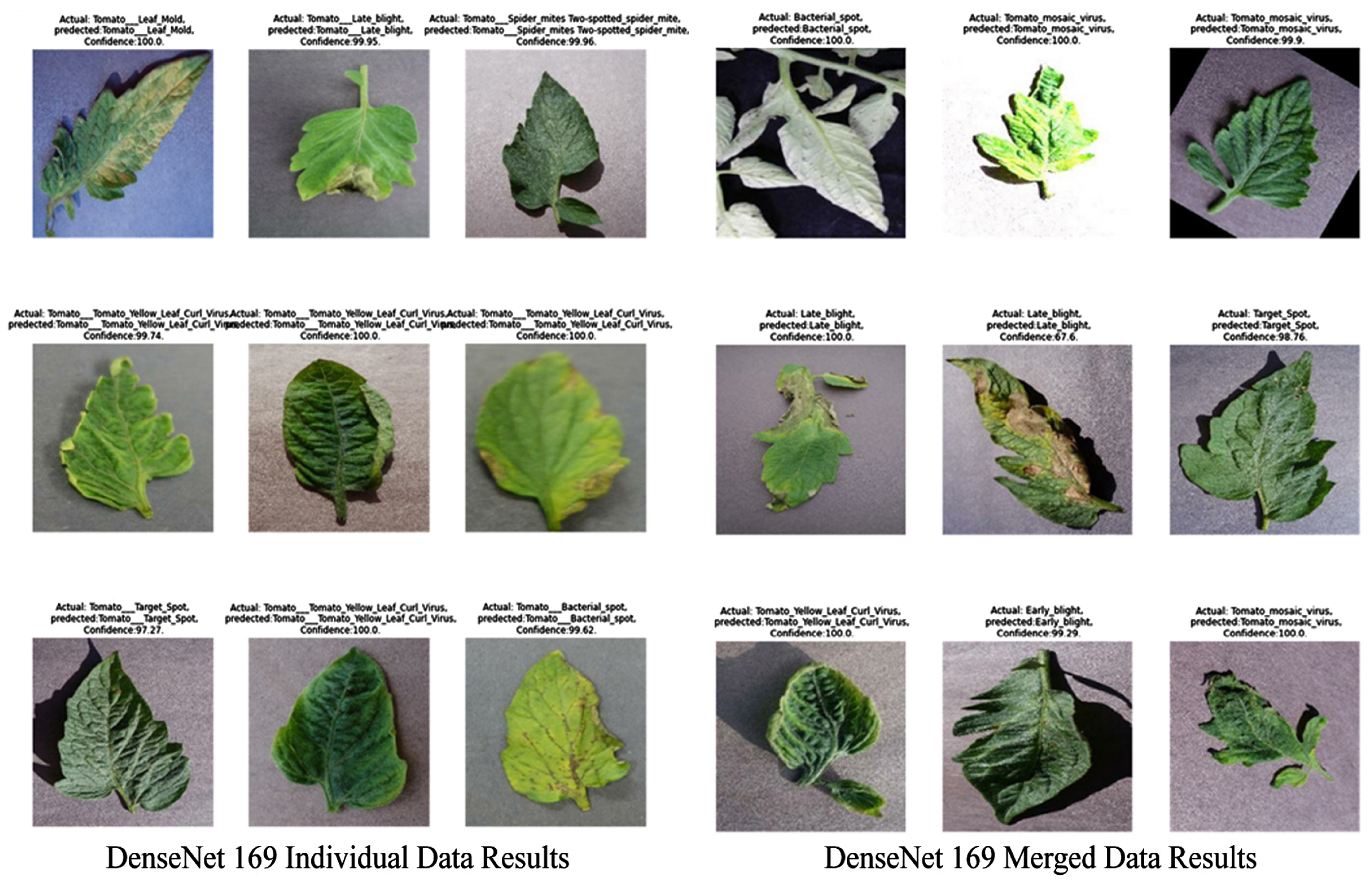
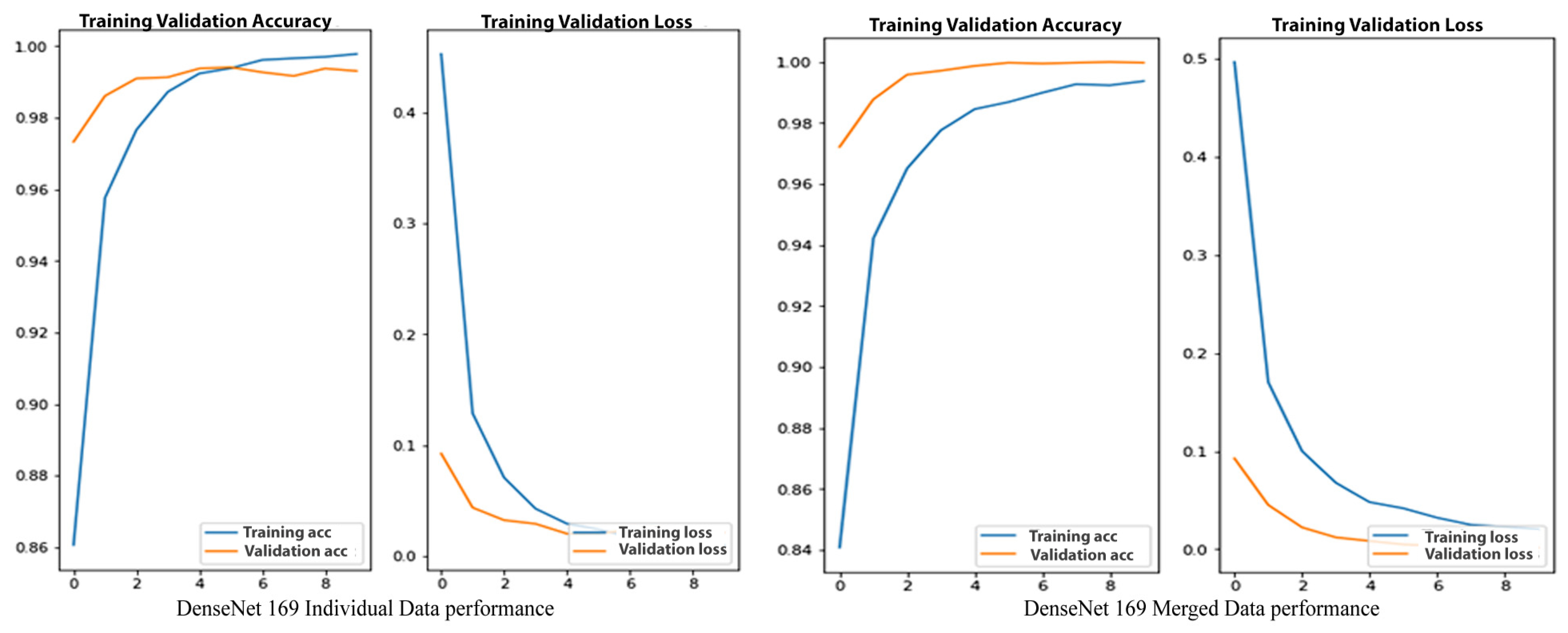
4.5. DenseNet169
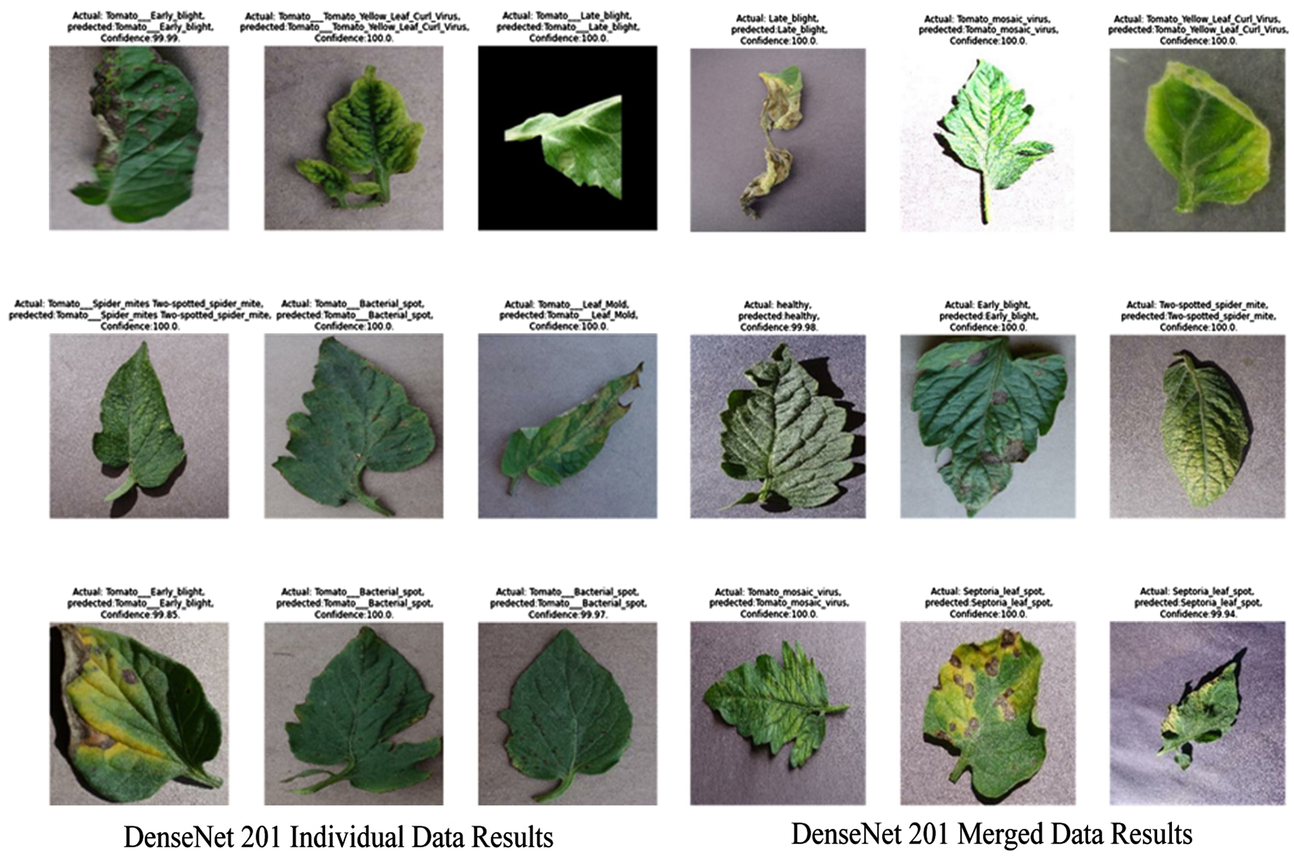
4.6. DenseNet201
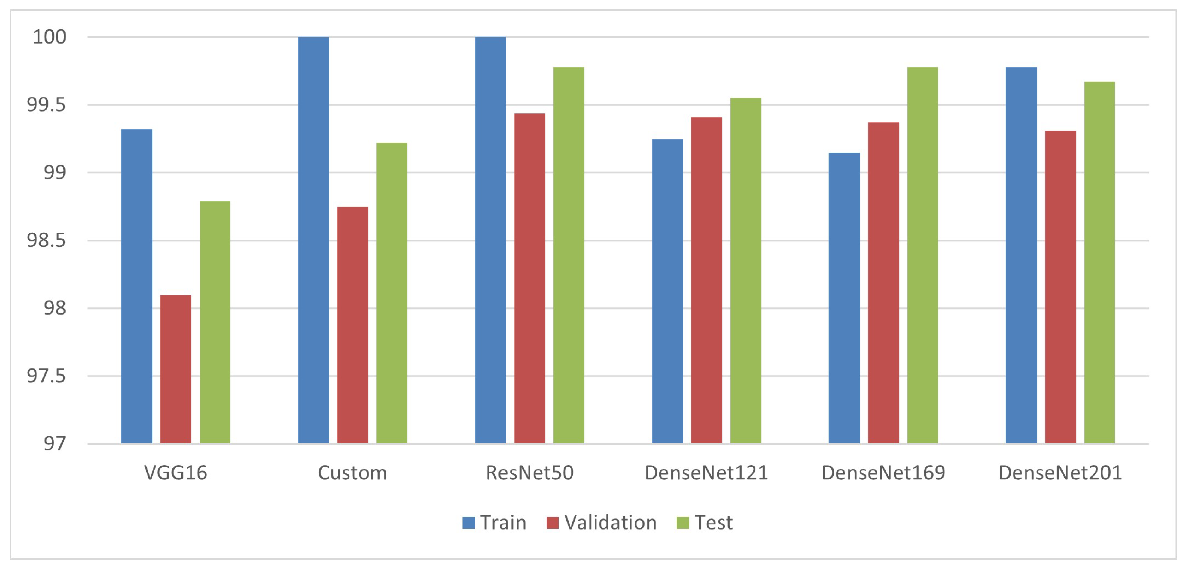
5. Comparative Analysis and Discussions
5.1. Comparison Table of Individual Data
5.2. Comparison Chart of Individual Data
5.3. Comparison Table of Merged Data
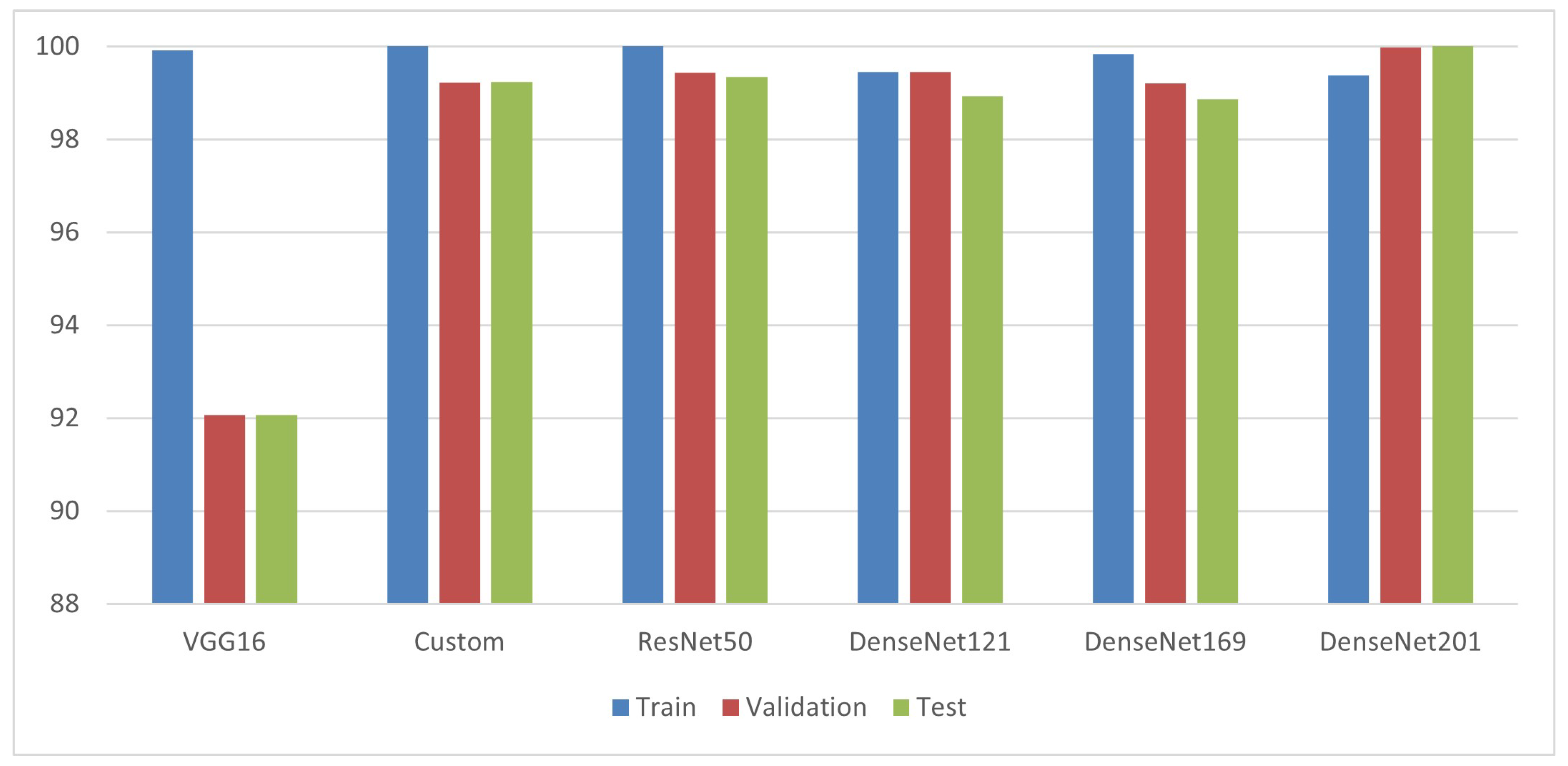
5.4. Comparison Chart of Merged Data
6. Conclusions and Future Work
Author Contributions
Funding
Data Availability Statement
Conflicts of Interest
References
- Punitha, K.; Shrivastava, G. Review on Emerging Trends in Detection of Plant Diseases using Image Processing with Machine Learning. Int. J. Comput. Appl. 2021, 174, 39–48. [Google Scholar]
- Andreas, K.; Prenafeta-Boldú, F.X. A review of the use of convolutional neural networks in agriculture. J. Agric. Sci. 2018, 156, 312–322. [Google Scholar]
- Sukhvir, K.; Pandey, S.; Goel, S. Plants disease identification and classification through leaf images: A survey. Arch. Comput. Methods Eng. 2019, 26, 507–530. [Google Scholar]
- Kumar, S.S.; Raghavendra, B.K. Diseases detection of various plant leaf using image processing techniques: A review. In Proceedings of the 5th International Conference on Advanced Computing & Communication Systems (ICACCS), Coimbatore, India, 15–16 March 2019; pp. 313–316. [Google Scholar]
- Arnal, B.J.G. Impact of dataset size and variety on the effectiveness of deep learning and transfer learning for plant disease classification. Comput. Electron. Agric. 2018, 153, 46–53. [Google Scholar]
- Devanur, G.; Mallikarjuna, P.B.; Manjunath, S. Segmentation and classification of tobacco seedling diseases. In Proceedings of the Fourth Annual ACM Bangalore Conference, Bangalore, India, 25–26 March 2011; pp. 1–5. [Google Scholar]
- Konstantinos, F. Deep learning models for plant disease detection and diagnosis. Comput. Electron. Agric. 2018, 145, 311–318. [Google Scholar]
- Hammad, S.M.; Potgieter, J.; Arif, K.M. Plant disease classification: A comparative evaluation of convolutional neural networks and deep learning optimizers. Plants 2020, 9, 1319. [Google Scholar]
- Punitha, K.; Shrivastava, G. Analytical study of deep learning architectures for classification of plant diseases. J. Algebr. Stat. 2022, 13, 907–914. [Google Scholar]
- Amarjeeth, S.; Jaisree, H.; Aishwarya, D.; Jayasree, J.S. Plant disease detection and diagnosis using deep learning. In Proceedings of the International Conference for Advancement in Technology (ICONAT), Goa, India, 21–22 January 2022; pp. 1–6. [Google Scholar]
- Vishakha, K.; Munot, M. Deep learning models for tomato plant disease detection. In Advanced Machine Intelligence and Signal Processing; Springer: Singapore, 2022; pp. 679–686. [Google Scholar]
- Khalil, K.; Khan, R.U.; Albattah, W.; Qamar, A.M. End-to-end semantic leaf segmentation framework for plants disease classification. Complexity 2022, 55, 1076–2787. [Google Scholar]
- Wadadare, S.S.; Fadewar, H.S. Deep learning convolution neural network for tomato leaves disease detection by inception. In Applied Computational Technologies: Proceedings of ICCET; Springer: Singapore, 2022; pp. 208–220. [Google Scholar]
- Chen, H.-C.; Widodo, A.M.; Wisnujati, A.; Rahaman, M.; Lin, J.C.-W.; Chen, L.; Weng, C.-E. AlexNet convolutional neural network for disease detection and classification of tomato leaf. Electronics 2022, 11, 951. [Google Scholar] [CrossRef]
- Khan, M.A.; Alqahtani, A.; Khan, A.; Alsubai, S.; Binbusayyis, A.; Ch, M.M.I.; Yong, H.-S.; Cha, J. Cucumber leaf diseases recognition using multi-level deep entropy-ELM feature selection. Appl. Sci. 2022, 12, 593. [Google Scholar] [CrossRef]
- Yiting, X.; Plett, D.; Liu, H. Detecting crown rot disease in wheat in controlled environment conditions using digital color imaging and machine learning. AgriEngineering 2022, 4, 141–155. [Google Scholar]
- Kaur, P.; Harnal, S.; Tiwari, R.; Upadhyay, S.; Bhatia, S.; Mashat, A.; Alabdali, A.M. Recognition of leaf disease using hybrid convolutional neural network by applying feature reduction. Sensors 2022, 22, 575. [Google Scholar] [CrossRef] [PubMed]
- Almadhor, A.; Rauf, H.T.; Lali MI, U.; Damaševičius, R.; Alouffi, B.; Alharbi, A. AI-driven framework for recognition of guava plant diseases through machine learning from DSLR camera sensor based high resolution imagery. Sensors 2021, 21, 3830. [Google Scholar] [CrossRef] [PubMed]
- Applalanaidu, M.V.; Kumaravelan, G. A review of machine learning approaches in plant leaf disease detection and classification. In Proceedings of the Third International Conference on Intelligent Communication Technologies and Virtual Mobile Networks (ICICV), Tirunelveli, India, 4–6 February 2021; pp. 716–724. [Google Scholar]
- Satheesh, S.B.P.; Naidu, P.R.S.; Neelima, U. Prediction of guava plant diseases using deep learning. In Proceedings of the 3rd International Conference on Communications and Cyber Physical Engineering (ICCCE), Hyderabad, India, 9–10 April 2021; pp. 1495–1505. [Google Scholar]
- Murat, T.; Arslan, R.S. RT-Droid: A novel approach for real-time android application analysis with transfer learning-based CNN models. J. Real-Time Image Process. 2023, 20, 55. [Google Scholar]


| Visual Geometry Group 16 Individual Data | Visual Geometry Group 16 Merged Data | ||||||
|---|---|---|---|---|---|---|---|
| Accuracy | Loss | Val Accuracy | Val Loss | Accuracy | Loss | Val Accuracy | Val Loss |
| 98.96 | 0.0323 | 98.77 | 0.0448 | 99.41 | 0.0199 | 92.29 | 0.6432 |
| 98.76 | 0.0382 | 97.88 | 0.0709 | 99.80 | 0.0094 | 92.24 | 0.6590 |
| 98.90 | 0.0380 | 99.15 | 0.0295 | 99.95 | 0.0015 | 91.95 | 0.6751 |
| 99.24 | 0.0271 | 97.95 | 0.0784 | 99.82 | 0.0058 | 92.11 | 0.6922 |
| 99.32 | 0.0200 | 98.10 | 0.0618 | 99.91 | 0.0037 | 92.06 | 0.6915 |
| Custom Model Individual Data | Custom Model Merged Data | ||||||
|---|---|---|---|---|---|---|---|
| Accuracy | Loss | Val Accuracy | Val Loss | Accuracy | Loss | Val Accuracy | Val Loss |
| 100 | 1.7998 × 10⁻⁴ | 98.78 | 0.0483 | 95.86 | 0.1574 | 70.52 | 1.4740 |
| 100 | 1.2213 × 10⁻⁴ | 98.78 | 0.0481 | 99.72 | 0.0110 | 79.61 | 1.0076 |
| 100 | 9.4443 × 10⁻⁵ | 98.82 | 0.0486 | 99.96 | 0.0032 | 99.01 | 0.0328 |
| 100 | 7.4930 × 10⁻⁵ | 98.89 | 0.0497 | 100 | 0.0012 | 99.11 | 0.0355 |
| 100 | 6.0184 × 10⁻⁵ | 98.75 | 0.0487 | 100 | 9.1173 × 10⁻⁴ | 99.22 | 0.0289 |
| ResNet Individual Data | ResNet Merged Data | ||||||
|---|---|---|---|---|---|---|---|
| Accuracy | Loss | Val Accuracy | Val Loss | Accuracy | Loss | Val Accuracy | Val Loss |
| 99.99 | 5.2742 × 10⁻⁴ | 99.44 | 0.0196 | 100 | 1.6210 × 10⁻⁴ | 99.48 | 0.0282 |
| 100 | 2.0346 × 10⁻⁴ | 99.44 | 0.0191 | 100 | 1.6100 × 10⁻⁴ | 99.43 | 0.0286 |
| 100 | 1.5636 × 10⁻⁴ | 99.44 | 0.0191 | 100 | 1.5992 × 10⁻⁴ | 99.45 | 0.0285 |
| 100 | 1.3528 × 10⁻⁴ | 99.44 | 0.0190 | 100 | 1.5885 × 10⁻⁴ | 99.48 | 0.0285 |
| 100 | 1.2024 × 10⁻⁴ | 99.44 | 0.0192 | 100 | 1.5780 × 10⁻⁴ | 99.45 | 0.0284 |
| DenseNet 121 Individual Data | DenseNet121 Merged Data | ||||||
|---|---|---|---|---|---|---|---|
| Accuracy | Loss | Val Accuracy | Val Loss | Accuracy | Loss | Val Accuracy | Val Loss |
| 98.26 | 0.0547 | 98.96 | 0.0319 | 98.75 | 0.0420 | 99.40 | 0.0207 |
| 98.69 | 0.0439 | 99.27 | 0.0277 | 99.05 | 0.0328 | 99.43 | 0.0219 |
| 99.00 | 0.0348 | 99.24 | 0.0225 | 99.22 | 0.0274 | 99.45 | 0.0207 |
| 99.10 | 0.0300 | 99.31 | 0.0211 | 99.46 | 0.0213 | 99.37 | 0.0218 |
| 99.25 | 0.0272 | 99.41 | 0.0203 | 99.46 | 0.0193 | 99.24 | 0.0209 |
| Dense Net 169 Individual Data | DenseNet169 Merged Data | ||||||
|---|---|---|---|---|---|---|---|
| Accuracy | Loss | Val Accuracy | Val Loss | Accuracy | Loss | Val Accuracy | Val Loss |
| 98.49 | 0.0470 | 99.13 | 0.0331 | 99.57 | 0.0184 | 98.95 | 0.0346 |
| 98.84 | 0.0371 | 99.20 | 0.0280 | 99.65 | 0.0161 | 98.87 | 0.0388 |
| 99.12 | 0.0296 | 99.20 | 0.0283 | 99.61 | 0.0141 | 98.87 | 0.0374 |
| 99.15 | 0.0266 | 99.37 | 0.0246 | 99.75 | 0.0112 | 98.98 | 0.0368 |
| 99.40 | 0.0205 | 99.34 | 0.0273 | 99.84 | 0.0092 | 99.02 | 0.0358 |
| Dense Net 201 Individual Data | DenseNet201 Merged Data | ||||||
|---|---|---|---|---|---|---|---|
| Accuracy | Loss | Val Accuracy | Val Loss | Accuracy | Loss | Val Accuracy | Val Loss |
| 99.38 | 0.0240 | 99.41 | 0.0201 | 98.69 | 0.0418 | 99.97 | 0.0050 |
| 99.61 | 0.0171 | 99.27 | 0.0235 | 98.99 | 0.0322 | 99.95 | 0.0036 |
| 99.66 | 0.0148 | 99.17 | 0.0233 | 99.27 | 0.0250 | 99.97 | 0.0021 |
| 99.70 | 0.0131 | 99.37 | 0.0191 | 99.24 | 0.0229 | 100 | 0.0019 |
| 99.78 | 0.0098 | 99.31 | 0.0211 | 99.37 | 0.0204 | 99.97 | 0.0018 |
| Model | Optimizer | Layers | Parameters | No. of Epochs | Training Accuracy | Training Loss | Validation Accuracy | Validation Loss | Test Accuracy |
|---|---|---|---|---|---|---|---|---|---|
| VGG16 | Adamax | 16 | 27,514,698 | 30 | 99.32% | 0.0200 | 98.10% | 0.0618 | 98.79% |
| Custom | Adamax | 10 | 8,598,090 | 30 | 100% | 6.0618 × 10⁵ | 98.75% | 0.0487 | 99.22% |
| ResNet 50 | SGD | 50 | 6,315,018 | 10 | 100% | 1.202 × 10⁴ | 99.44 | 0.0203 | 99.78% |
| DenseNet121 | SGD | 121 | 51,914,250 | 10 | 99.25% | 0.0272 | 99.41% | 0.0203 | 99.55% |
| DenseNet169 | SGD | 169 | 84,028,170 | 05 | 99.15% | 0266 | 99.37% | 0.0246 | 99.78% |
| DenseNet201 | SGD | 201 | 96,873,738 | 05 | 99.78% | 0098 | 99.31% | 0.0211 | 99.67% |
| Model | Optimizer | Layers | Parameters | Training Accuracy | Training Loss | Validation Accuracy | Validation Loss | Test Accuracy |
|---|---|---|---|---|---|---|---|---|
| VGG16 | Adamax | 16 | 27,514,698 | 99.91% | 0.0037 | 92.06% | 0.6915 | 92.06% |
| Custom | Adamax | 14 | 8,598,090 | 100% | 9.1173 × 10⁻⁴ | 99.22% | 0.0289 | 99.24% |
| ResNet 50 | SGD | 50 | 6,315,018 | 100% | 1.5780 × 10⁻⁴ | 99.45% | 0.0284 | 99.34% |
| Dense Net121 | SGD | 121 | 51,914,250 | 99.46% | 0.0193 | 99.24% | 0.0209 | 98.93% |
| Dense Net169 | SGD | 169 | 84,028,170 | 99.84% | 0.0092 | 99.02% | 0.0358 | 98.87% |
| Dense Net201 | SGD | 201 | 96,873,738 | 99.37% | 0.0204 | 99.97% | 0.0018 | 100% |
Disclaimer/Publisher’s Note: The statements, opinions and data contained in all publications are solely those of the individual author(s) and contributor(s) and not of MDPI and/or the editor(s). MDPI and/or the editor(s) disclaim responsibility for any injury to people or property resulting from any ideas, methods, instructions or products referred to in the content. |
© 2024 by the authors. Licensee MDPI, Basel, Switzerland. This article is an open access article distributed under the terms and conditions of the Creative Commons Attribution (CC BY) license (https://creativecommons.org/licenses/by/4.0/).
Share and Cite
Islam, S.U.; Zaib, S.; Ferraioli, G.; Pascazio, V.; Schirinzi, G.; Husnain, G. Enhanced Deep Learning Architecture for Rapid and Accurate Tomato Plant Disease Diagnosis. AgriEngineering 2024, 6, 375-395. https://doi.org/10.3390/agriengineering6010023
Islam SU, Zaib S, Ferraioli G, Pascazio V, Schirinzi G, Husnain G. Enhanced Deep Learning Architecture for Rapid and Accurate Tomato Plant Disease Diagnosis. AgriEngineering. 2024; 6(1):375-395. https://doi.org/10.3390/agriengineering6010023
Chicago/Turabian StyleIslam, Shahab Ul, Shahab Zaib, Giampaolo Ferraioli, Vito Pascazio, Gilda Schirinzi, and Ghassan Husnain. 2024. "Enhanced Deep Learning Architecture for Rapid and Accurate Tomato Plant Disease Diagnosis" AgriEngineering 6, no. 1: 375-395. https://doi.org/10.3390/agriengineering6010023
APA StyleIslam, S. U., Zaib, S., Ferraioli, G., Pascazio, V., Schirinzi, G., & Husnain, G. (2024). Enhanced Deep Learning Architecture for Rapid and Accurate Tomato Plant Disease Diagnosis. AgriEngineering, 6(1), 375-395. https://doi.org/10.3390/agriengineering6010023